Scaling theory in a model of corrosion and passivation

Abstract

We study a model for corrosion and passivation of a metallic surface after small damage of its protective layer using scaling arguments and simulation. We focus on the transition between an initial regime of slow corrosion rate (pit nucleation) to a regime of rapid corrosion (propagation of the pit), which takes place at the so-called incubation time. The model is defined in a lattice in which the states of the sites represent the possible states of the metal (bulk, reactive and passive) and the solution (neutral, acidic or basic). Simple probabilistic rules describe passivation of the metal surface, dissolution of the passive layer, which is enhanced in acidic media, and spatially separated electrochemical reactions, which may create pH inhomogeneities in the solution. On the basis of a suitable matching of characteristic times of creation and annihilation of pH inhomogeneities in the solution, our scaling theory estimates the average radius of the dissolved region at the incubation time as a function of the model parameters. Among the main consequences, that radius decreases with the rate of spatially separated reactions and the rate of dissolution in acidic media, and it increases with the diffusion coefficient of $H^{+}$ and ${OH}^{-}$ ions in solution. The average incubation time can be written as the sum of a series of characteristic times for the slow dissolution in neutral media, until significant pH inhomogeneities are observed in the dissolved cavity. Despite having a more complex dependence on the model parameters, it is shown that the average incubation time linearly increases with the rate of dissolution in neutral media, under the reasonable assumption that this is the slowest rate of the process. Our theoretical predictions are expected to apply in realistic ranges of values of the model parameters. They are confirmed by numerical simulation in two-dimensional lattices, and the expected extension of the theory to three dimensions is discussed.

I Introduction

The corrosion of a metal after the damage of its protective layer is a problem of wide technological interest. The evolution of the corrosion front is the result of a competition between localized dissolution and passivation processes. The latter consists of the formation of a passivation layer which reduces the corrosion rate and prevents a fast propagation of the damage. However, the breakdown of the passivation layer leads to the so-called pitting corrosion frankel , with an increase in the dissolution rate. It is generally accepted that the propagation of the pit is preceded by a nucleation regime, and the transition between these regimes takes place at the so-called pit initiation time or incubation time. This characteristic time was experimentally observed for a long time hoar ; shibata . In stainless steel, the process is often connected with the presence of inclusions ($MnS$) from which the pits begin alkire . In weakly passivated materials, it often begins at surface defects and surface inhomogeneities frankel , with only a small fraction giving rise to indefinitely developing pits. Some recent works determined relations between the incubation times and physicochemical conditions in different processes of technological interest (see. e. g. Refs. fukumoto ; hassan ; rehim ; amin ; zaky ).

There is also extensive literature covering the theoretical aspects of pitting corrosion. In some cases, specific applications are considered, such as stainless steel nagatani1 ; laycock1 ; laycock2 , while some works focus on universal features of that process meakin1 . Among the models we may also distinguish the ones based on stochastic approaches nagatani1 ; meakin1 ; nagatani2 ; nagatani3 ; meakin2 from those based on analytical formulations of the corrosion problem laycock1 ; laycock2 ; digby ; organ . These papers are devoted to the study of pit propagation, with the focus on the pit shapes laycock1 ; meakin2 ; nagatani3 and their evolution or the investigation of the interaction between pits organ .

On the other hand, the transition between the nucleation regime and pit propagation has attracted less attention. It motivated the recent study of a stochastic model with mechanisms that may be involved in this transition vautrin1 ; stafiej ; passivity . These mechanisms are passivation/depassivation phenomena, generation of local pH inhomogeneities by spatially separated cathodic and anodic reactions and smoothing out of these inhomogeneities by diffusion. Simulation of the corrosion process initiated by small damage to a protective surface showed the existence of an incubation time separating a nucleation regime of slow corrosion from a regime with a much higher growth rate of the corrosion front. Qualitative features of the growing cavities in two-dimensional simulations have already been addressed vautrin1 ; stafiej . However, a thorough analysis of the quantitative effects of different model parameters is still lacking.

In this paper, we extend the study of this corrosion model by combining scaling ideas and simulation results. Since the number of parameters of the original model is large, our study focuses on their values in the most realistic ranges for possible applications. Thus, while keeping the model amenable for a combination of theoretical and numerical work, we attempt to preserve the perspective of applications. The damage is represented by two lattice sites initially exposed to the environment, which mimics local damage of a relatively cheap (not stainless steel) painted material in its natural environment. This is certainly a situation of practical interest.

The starting point of our scaling analysis is to estimate the characteristic times of the physicochemical mechanisms involved in the corrosion process. By a suitable matching of those characteristic times, we estimate the incubation radius, which is defined as the effective radius of the dissolved region at the incubation time. Such a procedure resembles those recently used to estimate crossover exponents in statistical growth models rdcor ; lam . The incubation radius is related to model parameters such as probabilities of spatially separated reactions (cathodic and anodic), probabilities of acidity-enhanced depassivation and the diffusion coefficients. Subsequently, the dependence of the average incubation time on the model parameters is also analyzed. The theoretical predictions are supported by simulation data for two dimensional square lattices. This dimensionality is forced by computational limitations. However, the physicochemical and geometrical arguments of the theoretical analysis are independent of the underlying lattice structure. Thus we expect that this independence extends to the results in a certain range of the model parameters. This is important to justify the reliability of the model for a mesoscopic description of corrosion phenomena.

The paper is organized as follows. In Sec. II we review the statistical model and give a summary of the results of previous papers. In Sec. III we present the scaling theory for the model, which predicts the average radius of the dissolved cavity at the incubation time. In Sec. IV we compare the theoretical predictions with simulation data. In Sec. V we discuss the scaling properties of the incubation time. In Sec. VI we discuss the relations of this model with other reaction-diffusion models and other models for pitting corrosion. In Sec. VII we summarize our results and present our conclusions.

II The corrosion model

II.1 The electrochemical basis of the model

In an acidic or neutral medium, the anodic dissolution of commonly used metallic material such as steel, iron and aluminum, can be described by the reaction

$$Me+H_{2}O\to{MeOH}_{aq}+e^{-}+H^{+},$$ (1)

where $Me$ represents the bulk metal material and ${MeOH}_{aq}$ represents products which may be composed of hydroxides, oxides and water. For example, the mechanisms of $Ni$ dissolution in acid phosphate solutions was recently discussed in Ref. munoz . However, the precise chemical nature of these products is not important for the model presented here, but only the assumption that they are detached from the corroding material and belong to its environment.

On the other hand, in a basic environment the surface is expected to repassivate. In other words, the chemical species produced there are adherent to the surface and compact enough to prevent further dissolution. We represent it by the reaction

$$Me+{OH}^{-}\to{MeOH}_{ads}+e^{-},$$ (2)

where ${MeOH}_{ads}$ refers to the adherent species forming the passive layer at the metal surface. In both cases the pH of the solution at the locus of the reaction decreases.

In acidic deoxygenated media the associated cathodic reaction is

$$H^{+}+e^{-}\to\frac{1}{2}H_{2},$$ (3)

while in a basic environment we have

$$H_{2}O+e^{-}\to\frac{1}{2}H_{2}+{OH}^{-}.$$ (4)

As expected, these reactions increase the local pH.

If anodic and cathodic reactions occur next to each other there is a mutual compensation of their effect on pH and eventual neutralization. Thus the pairs of reactions (1)-(3) (in neutral or acidic medium) or (2)-(4) (in basic medium) do not alter pH of the solution at a significant lengthscale. Consequently, they can be simply combined as: (1-3)

$$Me+H_{2}O\to{MeOH}_{aq}+\frac{1}{2}H_{2}$$ (5)

if the surrounding solution is acidic, or as (2-4)

$$Me+H_{2}O\to{MeOH}_{ads}+\frac{1}{2}H_{2}$$ (6)

if the surrounding solution is basic. Reaction (6), in which the oxidation of the metal is followed by the deposition of a passive species, is much more frequent than the reaction (5), in which the product of the corrosion immediately leaves the surface. In a neutral medium, the former also tends to be dominant.

However, the spreading of the electric signal in the metal is considered as instantaneous when compared to the other processes. Therefore oxidation (1 or 2) and reduction (3 or 4) may occur at distant points simultaneously. These spatially separated electrochemical (SSE) reactions change the local pH of the solution where they occur in favor of occurrence of the reactions of the same type at the location. On the other hand, pH inhomogeneities (local excess of $H^{+}$ over ${OH}^{-}$) may be suppressed by diffusion, which tends to reimpose uniformity and brings about neutralization.

Finally, it is also important to recall that the dissolution of the adsorbed species (${MeOH}_{ads}$ in the above reactions) is very slow in a neutral medium, and even more difficult in a basic one. For instance, simulation of corrosion on steel by $CO_{2}$ at a high pH nesic shows low diffusion rates, with the formation of very protective films. However, the dissolution is significantly enhanced in acidic medium, following the reaction

$${MeOH}_{ads}+H^{+}\to{Me}^{+}+H_{2}O.$$ (7)

As the anions ${Me}^{+}$ leave the surface, the metal is again exposed to the corrosion agents.

II.2 The statistical model

Here we rephrase the model of Ref. vautrin1 , which amounts to describing the above processes at a mesoscopic level. Metal and solution are represented in a lattice, whose sites may assume six different states. These states represent the presence of significant amounts of the most important chemical species, while the chemical reactions are represented by stochastic rules for the changes of those states after each time step.

The sites representing the bulk metal (unexposed to the corroding solution) are labeled M and called metal or M sites. The so-called R (reactive) sites represent the ”bare” metal exposed to the corrosive environment. We consider the passivation layer at these points permeable enough to allow for anodic dissolution of the metal. In contrast, the passivated regions, labeled P sites, represent sites covered with a passive layer which is compact enough to prevent their anodic dissolution. The other lattice sites, labeled E, A and B, denote the neutral environment, the acidic and basic regions, respectively (compared to previous work on this model vautrin1 ; stafiej ; passivity , label C is here replaced by B in order to make a clearer association with the basic character of the solution and emphasize the pH role).

The evolution of the corrosion process amounts to transformations of the interfacial sites (R and P) into solution sites (E, A or B), followed by the conversion into R sites of those M sites that are put in contact with the solution. This accounts for the displacement of the interface. In the following, we will use the label S to denote a surface site which can be either R or P.

The possible changes of site labels certainly depend on the pH of the surrounding solution. Thus, for a given S site, our pH related scale will be represented by the algebraic excess of A sites over B sites among the nearest neighbors. We denote it by $N_{exc}$, so that the pH decreases as $N_{exc}$ increases.

During the simulation of the process, SSE reactions, local vicinity reactions and depassivation reactions are performed in this order. For each type of reaction, the lists of R and/or P sites are looked up in random order, and the decision of each one to undergo that reaction is taken with a prescribed probability. These reactions are followed by a certain number of random steps of A and B particles in the solution and possible annihilation of their pairs. This series of events takes place in one time unit.

The first set of transformations of the lattice sites account for the SSE reactions. In one time unit, each R site may undergo an SSE reaction with a probability $p_{SSE}$. In neutral or acidic medium ($N_{exc}\geq 0$), reaction (1) is represented by

$$R\to A,$$ (8)

and in basic medium ($N_{exc}<0$), reaction (2) is represented by

$$R+B(nn)\to P+E(nn)$$ (9)

(here $(nn)$ refers to a B site which is neareast neighbor of the R site). Any of the above anodic reactions is possible only if there is another surface site (R or P) which can mediate the associated cathodic process. This corresponds to the electrochemical reactions (3-4), and is represented in the model by

$$S+A(nn)\to S+E(nn),$$ (10)

or

$$S+E(nn)\to S+B(nn).$$ (11)

If none of the S sites has a nearest neighbor A or E, then the cathodic reaction is impossible, and consequently, the anodic one does not occur.

Subsequently, the possibility of local reactions is examined in a random sweep of the lists of R and P sites. The covering of the metal by the passive layer in neutral or basic medium is represented by

$$R\to P.$$ (12)

We assume that it occurs with probability $1$ in basic medium ($N_{exc}<0$) and probability $p_{cor1}$ in neutral medium ($N_{exc}=0$). On the other hand, in acidic medium ($N_{exc}>0$), R sites may be immediately dissolved, which corresponds to the reaction

$$R\to E.$$ (13)

In order to account for the effects of increasing acidity, this process is assumed to occur with probability $p_{cor2}N_{exc}$, where $p_{cor2}$ is constant. Here we assume that $p_{cor2}\ll 1$, following the idea that R sites are preferably dissolved in an anodic reaction.

The last set of possible transformations in a time unit account for depassivation. It is assumed that this process is not possible in a basic medium ($N_{exc}<0$) and rather slow in a neutral medium, so that the transformation

$$P\to E$$ (14)

occurs with a small probability $p_{oxi}$ when $N_{exc}=0$. On the other hand, in order to represent the effect of aggressive anions (reaction 7) in acidic medium ($N_{exc}>0$), we assume that (14) occurs with probability ${p^{\prime}}_{oxi}N_{exc}$, where ${p^{\prime}}_{oxi}$ is constant, but not very small. In previous works on the model vautrin1 ; stafiej , a fixed value ${p^{\prime}}_{oxi}=1/4$ was used. However, this process plays an essential role in the crossover from slow to rapid corrosion, thus possible variations of its rate will be considered here.

Finally, to represent diffusion in the solution, the random walk of particles A and B is considered. During one time unit, each A and B particle tries to perform $N_{diff}$ steps to nearest neighbor sites. If the step takes that particle to a site with neutral solution (E), then the particles exchange their positions: $A_{1}+E_{2}\to E_{1}+A_{2}$ or $B_{1}+E_{2}\to E_{1}+B_{2}$, where indexes $1$ and $2$ refer to neighboring lattice sites. If the step takes an A particle to a site with a B particle or vice versa, then they are annihilated and both are replaced by E particles: $A_{1}+B_{2}\to E_{1}+E_{2}$. This represents the reestablishment of neutrality by diffusion of the local excess of $H^{+}$ and ${OH}^{-}$ and by mutual irreversible neutralization. In all other cases A and B particles remain at their position.

It is important to recall that the probabilities defined above, as well as $N_{diff}$, can be viewed as the time rates for the corresponding processes. If the lattice parameter is $a$, then the diffusion coefficient of the A and B particles is $a^{2}N_{diff}/2d$, where $d$ is the system dimensionality. To simplify and reduce the number of parameters we take equal diffusion coefficients for both species.

II.3 Initial conditions and values of the model parameters

Although this model can be investigated with several different initial conditions, one of the most interesting cases is the study of the corrosion process taking place after a small damage of a protective layer. This is the case when a painted metal surface is locally damaged, which puts the metal in contact with an aggressive environment. It frequently occurs in relatively cheap (not stainless steel) painted materials in their natural environment, thus it is of great practical interest to investigate corrosion in such conditions.

In the model, such damage can be represented by the passivation of two sites of the top layer of a metallic matrix, while it is assumed that all sites around the metal are inert, i. e. they cannot be dissolved. This initial condition is illustrated in Fig. 1a and will be explored by a scaling theory and numerical methods in the next sections.

The most rapid process in this corrosion problem is expected to be that for passivation of reactive regions in a neutral or basic medium (reaction 12). For this reason, the unit rate is associated to this event in the basic medium, and $p_{cor1}\lesssim 1$ is adopted. On the other hand, the passivation in acidic medium is difficult, which justifies the choice $p_{cor2}\ll 1$. In the simulations of this paper, we will consider $p_{cor1}=0.9$, and $p_{cor2}=0.02$ or $p_{cor2}=0.005$.

The slowest process is expected to be the dissolution of passivated regions in a neutral medium. Since it occurs with probability $p_{oxi}$ per unit time, the characteristic time of this process is $\tau\equiv 1/p_{oxi}\gg 1$. However, dissolution is enhanced in acidic medium, which justifies the use of ${p^{\prime}}_{oxi}\gg p_{oxi}$.

It is also reasonable to assume that $p_{SSE}\ll 1$, since this is the fraction of reactions which generate significant pH inhomogeneities. However, this is the mechanism responsible for the onset of high corrosion rates after an incubation time, which suggests that $p_{SSE}\ll p_{oxi}$. Otherwise, the effective rate of metal dissolution would not be affected by the pH inhomogeneities.

Finally, diffusion rates of particles A and B are also of order $1$ or larger, which accounts for rapid cancellation of pH fluctuations in the solution.

II.4 Summary of previous results on the model

The above model without the SSE reactions was formerly considered in Ref. vautrin , where the evolution of the corrosion front was analyzed via simulations and a mean-field approach. The first study of the corrosion model with SSE reactions was presented in Ref. vautrin1 , where the formation of domains of A and B particles in a highly irregular dissolved region was observed, as well as the existence of a nucleation regime before the rapid pit propagation.

The first study which focused the nucleation regime was presented in Ref. stafiej , where the distribution of incubation times was obtained from simulation. It was shown that, at short times, the size of the dissolved region slowly increased because the rates of dissolution of P particles were very small and the repassivation of reactive sites was very frequent. The products of anodic and cathodic reactions create inhomogeneities in the local pH of the solution, represented by A and B particles, but these particles mutually neutralize in an $A+B\rightarrow 0$ reaction. These features characterize the nucleation regime.

However, anodic and cathodic reactions may occur at two distant points, which makes the neutralization slow, while the regions enriched in anions are noxious for repassivation, promoting further dissolution of the metal. Consequently, after a certain time the size of the cavity and the number of A and B particles rapidly increase. This corresponds to the onset of pitting corrosion. The distribution of incubation times characterizing the transition from the nucleation regime to pitting corrosion was obtained in Ref. stafiej for two different values of the model parameters. It was shown that the average incubation time decreased as $p_{oxi}$ increased, but no the study of the relations between incubation time and the other model parameters was presented there.

III Scaling theory

Starting from the configuration in Fig. 1a, one of the initial P sites is dissolved after a characteristic time of order $\tau/2$ (reaction 14). It leads to the appearance of reactive sites at its neighborhood, as illustrated in Fig. 1b for the case of depassivation of the P site at the left.

When $p_{SSE}=0$, the subsequent steps of the process are the passivation of the reactive sites, which leads to the configuration shown in Fig. 1c. Consequently, an additional time of order $\tau/3$ will be necessary for dissolution of a region of the passive layer in Fig. 1c and the onset of new reactive sites. After that, the new R sites will also be rapidly passivated. Thus, for small $p_{oxi}$ (large $\tau$), the corrosion process is always slow. A mean-field theory is able to predict its long-term behavior vautrin .

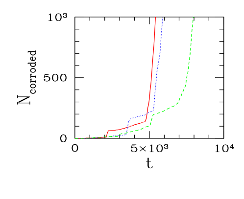
Figure 2: Number of dissolved sites as a function of time, obtained in three different realizations of the model. Parameter values are $p_{SSE}=0.02$, $p_{oxi}={10}^{-3}$, ${p^{\prime}}_{oxi}=0.25$, $p_{cor1}=0.9$, $p_{cor2}=0.02$, and $N_{diff}=1$.

The case of nonzero but small $p_{SSE}$ is much more complex due to the appearance of the pH inhomogeneities in the solution. Fig. 1d illustrates the result of an SSE reaction after the configuration of Fig. 1b, followed by diffusion which leads to the annihilation of the pair AB. Simulation of the model stafiej shows that, at short times, the size of the dissolved region increases and the region acquires the approximate shape of a semicircle centered at the point of the initial damage. After a certain time, the rate of production of A and B particles remarkably increases, compensating the annihilation effects. This is mainly a consequence of the enhanced dissolution and the impossibility of passivation in acidic regions. Consequently, the total rate of dissolution of the metal becomes much larger and the cavity develops an irregular shape. The time evolution of the area of the dissolved region (number of dissolved sites) obtained in simulation is illustrated in Fig. 2.

In order to relate the geometrical features of the dissolved cavity with the model parameters, we will consider that it has the semicircular shape of radius $R$ shown in Fig. 3. In the following, we will estimate the characteristic times for creation of new A and B particles in that cavity and the characteristic time for the annihilation of one of those pairs. Matching these time scales, we can predict conditions for the incubation to occur. This reasoning follows the same lines which are successfully applied to study the crossover between different growth kinetics in Ref. rdcor .

First we consider the mechanisms for depassivation followed by SSE reactions. There are two possible paths for the dissolution of particles P and creation of new reactive sites: dissolution in a neutral environment, with probability $p_{oxi}$, and dissolution in acidic medium, i. e. in contact with A particles, which typically occurs with probability ${p^{\prime}}_{oxi}$ (contact with a single A particle). In any case, the generation of a new particle A requires a subsequent SSE reaction.

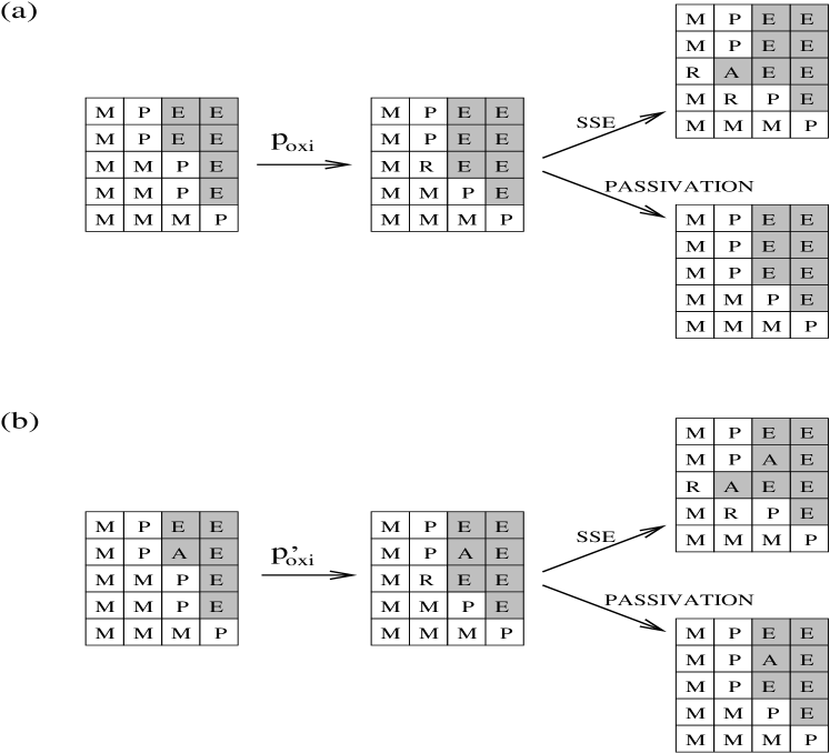
Figure 4: (a) Scheme showing a region of the surface of the cavity where dissolution in neutral medium occurs, followed by SSE reactions or by passivation of reactive sites. The solution sites are shaded in order to illustrate the evolution of the front. (b) The same scheme with dissolution in acidic medium, i. e. dissolution of a P site with a neighboring A.

In the case of dissolution in a neutral environment, the average time necessary for dissolution of a single P particle is $\tau/N_{P}$, where $N_{P}$ is the current number of P particles at the surface of the cavity. This is illustrated in Fig. 4a. After dissolution, one or two R particles are generated, and each one may undergo an SSE reaction with probability $p_{SSE}$. Otherwise, these R particles are rapidly passivated, and new SSE reactions will be possible only after another depassivation event. These two possibilities are also illustrated in Fig. 4a. Thus, the average time for creation of a pair AB inside the cavity from this path is of order $\tau_{cre}\sim\tau/N_{P}/p_{SSE}$. While $\tau$ must be interpreted as a time interval, here $p_{SSE}$ must be viewed as a dimensionless probability which indicates the fraction of depassivation events that are followed by SSE reactions. Now, since $N_{P}$ is of the order of the number of sites at the surface of the cavity, we have

$$N_{P}\sim\pi R/a$$ (15)

for the cavity of radius $R$ (Fig. 3 - $a$ is the lattice parameter). This leads to

$$\tau_{cre}\sim\frac{\tau a}{\pi Rp_{SSE}}.$$ (16)

In the case of dissolution in an acidic environment, we assume that there is an A particle present in the cavity. The fraction of the time it spends in the surface of the cavity is approximately the ratio between the number of perimeter sites and the total number of sites in the cavity (Fig. 3): $\left(\pi R/a\right)/\left(\pi R^{2}/2a^{2}\right)=2a/R$. The probability of dissolution of P in contact with a single A is ${p^{\prime}}_{oxi}$, thus the characteristic time for dissolution is $1/{p^{\prime}}_{oxi}$ in this case. This process is illustrated in Fig. 4b. Again, the subsequent processes may be SSE reactions or passivation of the R particles (see Fig. 4b). Thus, the average time for production of a new A particle is

$${\tau^{\prime}}_{cre}\sim\frac{1}{2a/R}\frac{1}{{p^{\prime}}_{oxi}}\frac{1}{p_{SSE}}=\frac{R}{2a{p^{\prime}}_{oxi}p_{SSE}}$$ (17)

Again, in this case $p_{SSE}$ must be viewed as a dimensionless fraction of SSE reactions.

Certainly the above estimates of $\tau_{cre}$ and ${\tau^{\prime}}_{cre}$ contain inexact numerical factors, but the dependence on the model parameters is expected to be captured. However, it is interesting to stress that the superestimation of ${\tau^{\prime}}_{cre}$ not only comes from geometrical aspects but also from diffusion. Indeed, the random movement of the A particle tends to be slower in contact with the surface, where the number of empty neighbors is smaller. This increases the average time of A in contact with P.

Now we estimate the characteristic time for annihilation of a pair of particles A and B, which represents the smoothing out of local pH inhomogeneities and leads to a decrease of the dissolution rate. Such a pair is illustrated in Fig. 3. In a first approximation we expect that the average time for its annihilation, $\tau_{ann}$, is of the order of the number of sites inside the cavity divided by the number of steps per time unit, $N_{diff}$. Thus

$$\tau_{ann}\sim\frac{\left(R^{2}/2a^{2}\right)}{N_{diff}}.$$ (18)

Notice that, when the cavity is small, $\tau_{ann}\ll{\tau^{\prime}}_{cre}\ll\tau_{cre}$, thus all pairs AB are rapidly annihilated after their production. It means that the solution is neutral during most of the time. This conclusion is realistic because, at large length scales, the solution is expected to always be neutral. However, as $R$ grows, the number of pairs AB in the cavity increases, which leads to a more rapid dissolution of the metal and slower smoothing out the of pH inhomogeneities. For sufficiently low probabilities $p_{oxi}$ of dissolution in a neutral medium, as discussed in Sec. II.3, we expect that $\tau_{cre}$ is always large compared to the other time scales. Thus, a series of reactions appears when dissolution in acidic medium becomes rapid enough to counterbalance the neutralizing effect of diffusion. At this time, if a new pair AB is created, it will induce the creation of other pairs and, consequently, a succession of SSE reactions. This is clear from Fig. 4b, in which we observe the production of two A particles in a small region of the lattice. Thus, at the incubation time, we expect that $\tau_{ann}\sim{\tau^{\prime}}_{cre}$. Using Eqs. (17) and (18), we obtain an average radius

$$R_{I}\sim\frac{N_{diff}}{\pi p_{SSE}{p^{\prime}}_{oxi}}\qquad,\qquad d=2,$$ (19)

where the index $I$ refer to incubation time and the spatial dimension $d$ is emphasized.

This result was derived for the model in two dimensions because our simulations were performed in these conditions. In a three-dimensional system, the dependence of ${\tau^{\prime}}_{cre}$ on $R$ does not change, since it is derived from a boundary to volume ratio. However, $\tau_{ann}$ may increase as $R^{3}$ instead of $R^{2}$ for a three-dimensional cavity, since that is the order of the number of sites. Consequently, Eq. (19) is expected to be changed to

$$R_{I}\sim\sqrt{\frac{N_{diff}}{p_{SSE}{p^{\prime}}_{oxi}}}\qquad,\qquad d=3.$$ (20)

Thus, independently of the system dimensionality, we observe that $R_{I}$ decreases as $p_{SSE}$ or ${p^{\prime}}_{oxi}$ increase.

One of the interesting points of these results is their independence on the lattice structure, which is important for comparisons between such a mesoscopic model and experimental results. In the following, we show that simulation data are in a good agreement with the predictions in two dimensions in the cases where the sizes of the cavities and incubation times are large enough for such a continuous description to apply. This adds more confidence to the extension of this theoretical analysis to three-dimensional systems.

IV Simulation results

Our simulations are performed in a square lattice of vertical and horizontal sizes $L=1000$, with the central sites of the top layer (largest $y$) initially labeled as P and the rest labeled as M (Fig. 1a). The process is interrupted before or when the corrosion front reaches the sides or bottom of the box. Typically one hundred independent runs have been performed for each set of the model parameters.

Following previous experience with simulation of this model, the incubation time is defined as that in which the number of particles A (or B) is 20. Although our scaling theory predicted the time necessary for the creation of the second A particle, it is observed that within a very narrow time interval the number of A and B particles rapidly increases from values near 2 or 3 to some tenths. Thus, defining the incubation time in the presence of a smaller numbers of particles A, such as 10 or 15, leaded to negligible changes in the final estimates of incubation times and radii of the cavities.

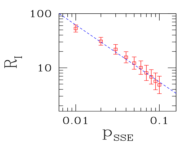
Figure 5: Incubation radius as a function of $p_{SSE}$, for small $p_{SSE}$, with $p_{oxi}={10}^{-3}$, ${p^{\prime}}_{oxi}=0.25$, $p_{cor1}=0.9$, $p_{cor2}=0.02$, and $N_{diff}=1$.

The first test of the relation (19) addresses the dependence of $R_{I}$ on $p_{SSE}$. Simulations for $0.01\leq p_{SSE}\leq 0.1$ are performed, considering fixed values of the other parameters: $p_{oxi}={10}^{-3}$, ${p^{\prime}}_{oxi}=0.25$, $p_{cor1}=0.9$, $p_{cor2}=0.02$, $N_{diff}=1$. In Fig. 5 we show a log-log plot of $R_{I}$ versus $p_{SSE}$ with a linear fit of slope $-1.05$. This is in a good agreement with Eq. (19) for constant ${p^{\prime}}_{oxi}$ and $N_{diff}$, which suggests $R_{I}\sim 1/p_{SSE}$. This is certainly the most important test to be performed with this model because it is much more difficult to estimate a relative probability of spatially separated reactions in an experiment than to measure diffusion coefficients or dissolution rates.

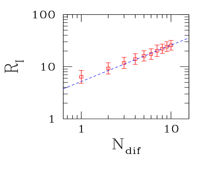
Figure 6: Incubation radius as a function of $N_{diff}$, with $p_{SSE}=0.1$, $p_{oxi}={10}^{-3}$, ${p^{\prime}}_{oxi}=0.25$, $p_{cor1}=0.9$, and $p_{cor2}=0.02$.

We also test the predicted dependence of $R_{I}$ on $N_{diff}$ by simulations with the same parameters above, except that we fix $p_{SSE}=0.1$ and $N_{diff}$ is varied between $1$ and $10$. In Fig. 6 we show a log-log plot of $R_{I}$ versus $N_{diff}$ with a linear fit of the data points with larger $N_{diff}$. That fit gives $R_{I}\sim{N_{diff}}^{0.7}$, which is a slightly slower dependence than the linear one predicted by Eq. (19). However, it illustrates the rapid increase of $R_{I}$ with the diffusion coefficient, and from Fig. 6 it is clear that the effective exponent in the relation between $R_{I}$ and $N_{diff}$ tends to increase as $N_{diff}$ increases effectiveexp . The deviation from the linear relation may be attributed, among other factors, to the assumption of free random walk properties for A and B particles in our scaling picture.

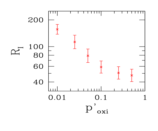
Figure 7: Incubation radius as a function of the probability of dissolution in acidic media, ${p^{\prime}}_{oxi}$, with $p_{SSE}=0.1$, $p_{oxi}={10}^{-3}$, $p_{cor1}=0.9$, $p_{cor2}=0.02$, and $N_{diff}=1$.

We also confirm that $R_{I}$ rapidly increases as ${p^{\prime}}_{oxi}$ decreases, particularly when the latter is small, as suggested by Eq. (19). We performed simulations with $p_{oxi}={10}^{-4}$, ${p}_{SSE}=0.01$, $p_{cor1}=0.9$, $p_{cor2}=0.02$, $N_{diff}=1$, and various ${p^{\prime}}_{oxi}$ between $0.25$ and $0.025$. In Fig. 7 we show a log-log plot of $R_{I}$ versus ${p^{\prime}}_{oxi}$. For small ${p^{\prime}}_{oxi}$ the incubation radius $R_{I}$ rapidly increases with decreasing ${p^{\prime}}_{oxi}$, although the exact dependence predicted in Eq. (19) is not observed. However, when ${p^{\prime}}_{oxi}$ is very small, the average time of creation of new A particles in acidic media (${\tau^{\prime}}_{cre}$) becomes very large and possibly comparable to the time for creation in neutral media ($\tau_{cre}$), even if $p_{oxi}$ is small. Consequently, a competition between these mechanisms may appear and rule out the above scaling picture.

Finally, we also test a possible dependence of $R_{I}$ on $p_{oxi}$. Simulations are performed with ${p^{\prime}}_{oxi}=0.25$, $p_{cor1}=0.9$, $p_{cor2}=0.02$, $N_{diff}=1$ and $p_{SSE}=0.1$, while $p_{oxi}$ varies between ${10}^{-2}$ and ${10}^{-4}$. The estimates of $R_{I}$ range between $9.67\pm 1.50$ and $9.87\pm 1.48$, i. e. they fluctuate $2\%$ while $p_{oxi}$ varies two orders of magnitude. This supports our prediction that $R_{I}$ does not depend on this rate. On the other hand, as discussed below, the average incubation time strongly depends on that quantity.

Another interesting point of our scaling analysis is the possibility of obtaining reliable estimates of the order of magnitude of the radius of the dissolved region at the incubation time. For instance, simulations with $p_{oxi}={10}^{-3}$, ${p^{\prime}}_{oxi}=0.25$, $p_{cor1}=0.9$, $p_{cor2}=0.02$, $N_{diff}=1$ and $p_{SSE}=0.01$ gave $R_{I}/a=53\pm 8$, while Eq. (19) gives $R_{I}=127$.

V Incubation time

Here we derive relations for the average incubation time by extending the analysis that leads to the scaling theory of Sec. III. Again, we focus on the ranges of realistic values of the model parameters presented in Sec. II.3.

The initial configuration of the system, shown in Fig. 1a, evolves to that shown in Fig. 1b after an average time $\tau/2$. The latter has a large probability [${\left(1-p_{SSE}\right)}^{2}$] of being passivated, which gives rise to the configuration with $3$ particles P of Fig. 1c. Otherwise, with a small probability of order $2p_{SSE}$, one of the R particles undergoes an SSE reaction, increasing the size of the dissolved region, as shown in Fig. 1d. However, due to the diffusion of A and B and the high probability of passivation of new R sites, there is a large probability that the first configuration of Fig. 1d evolves to passivated configurations with two or three E particles and four or five P particles. For instance, for $p_{sse}=0.1$, we estimate that nearly $80\%$ of the initial configurations will evolve to the passivated state of Fig. 1c, nearly $10\%$ will evolve to passivated states with four P and two E particles (last configuration of Fig. 1d with R replaced by P), and nearly $10\%$ will evolve to passivated states with five P and three E particles. The probability that A and B particles of the configuration in Fig. 1d survive and their number eventually increases is negligible.

Notice that the time intervals for diffusion of A and B particles and for the SSE reactions before passivation are both very small compared to $\tau$. Thus, the new passivated configurations described above are obtained after a time which is also approximately $\tau/2$, corresponding to the first dissolution event (process from Fig. 1a to Fig. 1b).

After repassivation of the surface, one of the P particles will be dissolved after a characteristic time of order $\tau/N_{P}$. From the above discussion, $N_{P}=3$ is the most probable value for small $p_{SSE}$ (Fig. 1b), although $N_{P}=4$ and $N_{P}=5$ have non-negligible probabilities of occurrence. Thus, new configurations with reactive sites will appear after the total time $\tau/2+\tau/N_{P}\left(2\right)$, where ${N_{P}\left(2\right)}$ is an average number of P particles before the second dissolution event (in neutral media). From the above discussion we see that ${N_{P}\left(2\right)}$ is slightly larger than 3 for small $p_{SSE}$ (${N_{P}\left(2\right)}=3$ for $p_{SSE}=0$).

Subsequently, passivation of reactive sites, diffusion and SSE reactions take place, but in all cases the time intervals are much smaller than $\tau$. New passive configurations will be generated, with larger $N_{P}$ and consequently, characteristic times $\tau/N_{P}$ to be depassivated (dissolution of one P). Thus, the average incubation time is expected to have the general form

$$\langle\tau_{INC}\rangle\approx\frac{\tau}{2}+\frac{\tau}{N_{P}\left(2\right)}+\frac{\tau}{N_{P}\left(3\right)}+\dots+\frac{\tau}{{N_{P}}^{INC}}.$$ (21)

Here, $N_{P}\left(i\right)$ is the average number of P particles in the passivated states just before the $i^{th}$ dissolution event, and ${N_{P}}^{INC}$ is the number of P particles at the time in which the rapid dissolution begins, i. e. at the incubation time. From Eq. (15), we have ${N_{P}}^{INC}\sim\pi R_{I}/a$, thus $R_{I}$ will determine the term where the series in Eq. (21) will be truncated.

This series resembles a harmonic series which is truncated at a certain term. Indeed, for very small $p_{SSE}$, the subsequent terms are expected to be close to consecutive integer values. Moreover, for $p_{SSE}=0$ the harmonic series is recovered and $\langle\tau_{INC}\rangle$ diverges, which is consistent with the fact that there is no incubation process without the SSE reactions vautrin .

One of the interesting features of the expansion in Eq. (21) is that it allows for the separation of the effects of the main chemical reactions and the effects of dissolution in neutral environment. While the former are important to determine $R_{I}$ (Eq. 19) and, consequently, the number of terms in the expansion, the latter determine the value of the characteristic time $\tau$. On the other hand, the sensitivity of $\langle\tau_{INC}\rangle$ on variations of $R_{I}$ is not high because the main contributions to the sum in Eq. (21) come from the terms with small $N_{P}$. Thus, significant variations in the incubation time are only expected from variations in the probability of dissolution in neutral medium, $p_{oxi}=1/\tau$. This is a somewhat expected feature because $\tau$ is the largest characteristic time of the relevant events in this system.

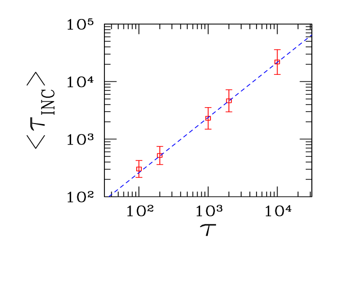
Figure 8: Average incubation time as a function of the oxidation time $\tau\equiv 1/p_{oxi}$, with $p_{SSE}=0.1$, ${p^{\prime}}_{oxi}=0.25$, $p_{cor1}=0.9$, $p_{cor2}=0.02$ and $N_{diff}=1$.

The above analysis is fully supported by our simulation data. In Fig. 8 we show a log-log plot of $\langle\tau_{INC}\rangle$ versus $\tau\equiv 1/p_{oxi}$, obtained in simulations with fixed values of the other parameters: ${p^{\prime}}_{oxi}=0.25$, $p_{cor1}=0.9$, $p_{cor2}=0.02$, $N_{diff}=1$, $p_{SSE}=0.1$. The linear fit of the data, shown in Fig. 8, has a slope $0.96$, which is very close to the value $1$ expected from Eq. (21) with constant denominators in all terms.

The above results imply that $\langle\tau_{INC}\rangle$ decreases as $p_{oxi}$ increases. Simulations of the model with different values of ${p^{\prime}}_{oxi}$, keeping the other parameters fixed, also show a decrease of $\langle\tau_{INC}\rangle$ as ${p^{\prime}}_{oxi}$ increases. On the other hand, both oxidation probabilities are expected to be enhanced by increasing the concentration of aggressive anions in solution. This parallels the experimental observation of a decrease in the incubation time as the concentration of those anions increases hassan ; rehim ; amin ; zaky , which shows the reliability of our model.

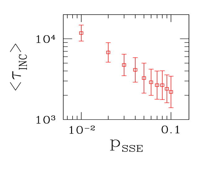
Figure 9: Average incubation time as a function of $p_{SSE}$, $p_{oxi}={10}^{-3}$, ${p^{\prime}}_{oxi}=0.25$, $p_{cor1}=0.9$, $p_{cor2}=0.02$ and $N_{diff}=1$.

In Fig. 9 we show $\langle\tau_{INC}\rangle$ versus $p_{SSE}$ obtained with the same set of parameters of the data as in Fig. 5. The observed dependence qualitatively agrees with Eq.(21): as $p_{SSE}$ increases, the radius $R_{I}$ decreases and, consequently, the number of terms in the series of Eq. (21) also decreases. However, due to the particular structure of Eq. (21), it is difficult to predict a simple relation between $\langle\tau_{INC}\rangle$ and $p_{SSE}$.

From Eq. (21) we are also able to provide the correct order of magnitude of the average incubation time. For instance, considering the simulation with $p_{oxi}={10}^{-3}$, ${p^{\prime}}_{oxi}=0.25$, $p_{cor1}=0.9$, $p_{cor2}=0.02$, $N_{diff}=1$ and $p_{SSE}=0.01$, we obtained $R_{I}/a\approx 53$ and $\langle\tau_{INC}\rangle\approx 1.2\times{10}^{4}$. On the other hand, using Eq. (15), that value of $R_{I}$ leads to ${N_{P}}^{INC}\approx 166$. Since $p_{SSE}$ is small, we may approximate the series in Eq. (21) by a harmonic series truncated at this value of ${N_{P}}^{INC}$, so that the theoretical estimate of incubation time is $4.7\times{10}^{3}$, i. e. of the same order of magnitude of the simulation value.

VI Relations to other corrosion models and reaction-diffusion systems

In our model, the crossover from slow corrosion to a rapid corrosion process takes place when regions with large number of A and B particles are produced in the solution. Indeed, previous simulation work on the model has already shown the presence of spatially separated domains of A and B particles in the solution vautrin1 after the incubation time, and this separation slows down the annihilation of A and B pairs.

This phenomenon resembles the segregation effects observed in reaction-diffusion systems of the type $A+B\to 0$ in confined media wilczek ; oz ; anacker ; lindenberg ; lin ; kopelman ; reigada , such as systems with tubular geometries and fractal lattices. In those systems, there is no injection of new particles and the initial distribution of reactants is random. However, after a certain time, large domains of A and B particles are found, and the annihilation process is possible only at the frontiers of those domains. Consequently, the concentration of A and B particles slowly decay when compared to the reactions of the type $A+A\to 0$ anacker ; lindenberg . As far as we know, this phenomenon was not experimentally observed yet, although the depletion zones of a related model ($A+B\to B$ reactions) were already observed in photobleaching of fluorescein dye by a focused laser beam trap1 ; trap2 .

However, the segregation is not expected for the reaction $A+B\to 0$ in three dimensions, and in two dimensions it is expected to be marginal lindenberg . This is the case in our model. The production of A and B particles takes place at the surface of the cavity, and this surface may play the same role of the rigid boundaries of confined media (restricting the diffusion of A and B particles) during a short times after their creation. However, the main mechanism contributing to segregation in our model is the preferential production of new A particles by dissolution in acidic media, i. e. production of new A particles close to the other A. Despite the differences in the mechanisms leading to segregation between our model and the reaction-diffusion systems of the type $A+B\to 0$, it is clear that in both cases the mixing of A and B domains is slow due to diffusion restrictions.

It is also important to notice that our model has significant differences from those of Refs. meakin1 ; meakin2 , which also aim at representing universal features of corrosion processes. They also consider the interplay between dissolution and passivation, with the former being limited by diffusion of an aggressive species in the solution. The concentration of the aggressive species depends only on the properties of the solution in contact with the metal. However, in our model the particles responsible for enhancing the dissolution (A and B, or pH inhomogeneities) are themselves dissolution products. This feature implies that the transition from the nucleation stage to pitting corrosion is a consequence of an auto-catalytic production of those particles. Instead, the models of Refs. meakin1 ; meakin2 and related stochastic models of pitting corrosion nagatani1 ; nagatani2 ; nagatani3 were suitable to represent features of the regime of pit propagation.

VII Discussion and conclusion

We studied a model for corrosion and passivation of a metallic surface after a small damage to its protective layer, in which an initial regime of slow corrosion crosses over at the incubation time to a regime of rapid corrosion. The dramatic increase of the corrosion rate is related to the presence of acidic regions in the solution and the autocatalytic enhancement of pH inhomogeneities due to spatially separated anodic and cathodic reactions. Our scaling analysis of the model is based on the matching of the characteristic times of creation and neutralization of pH inhomogeneities in the solution and leads to an estimate of the average radius $R_{I}$ of the dissolved region at the incubation time. That radius decreases with the rate of spatially separated reactions and the rate of dissolution in acidic media, and it increases with the diffusion coefficient of particles A and B in the solution, which tells us how fast the suppression of pH inhomogeneities takes place. The average incubation time is written as the sum of a series of characteristic times for the slow dissolution in neutral media. It has a complex dependence on $R_{I}$ and linearly increases with the rate of dissolution in neutral media. These results are confirmed by numerical simulation in two-dimensional lattices, but the extension of the theory to three dimensions is also discussed. Relations to other reaction-diffusion systems with segregation and other corrosion models are discussed. Since the relative values of the model parameters are expected to provide a realistic description of real corrosion processes, we believe that this work may be useful for the analysis of experimental work in this field.

Figure 1: (a) Initial configuration of the lattice, with two passivated sites in the top layer of the metallic matrix. (b) Configuration obtained after dissolution of the left P particle. (c) Configuration obtained after passivation of the R sites. (d) Configurations obtained after the leftmost R of (b) suffered an SSE reaction and after diffusion and annihilation of A and B.

Figure 3: Scheme of the cavity during the incubation process, assuming a semicircular shape. Most sites of the surface are passivated and particles A and B are allowed to diffuse in the cavity.

References

- (1) G. S. Frankel, J. Electrochem. Soc. 145, 2186 (1998).
- (2) T. P. Hoar and W. R. Jacob, Nature 216, 299 (1967).
- (3) T. Shibata and T. Takeyama, Nature 263, 315 (1976).
- (4) R. Alkire and M. Verhoff, Electrochim. Acta, 43, 2733 (1998).
- (5) M. Fukumoto, S. Maeda, S. Hayashi, and T. Narita, Oxidation of Metals 55, 401 (2001).
- (6) H. H. Hassan, S. S. A. El Rehim, and N. F. Muhamed, Corros. Science 44, 37 (2002).
- (7) S. S. A. El Rehim, E. E. F. El-Sherbini, and M. A. Amin, J. Electroanal. Chem. 560, 175 (2003).
- (8) M. A. Amin and S. S. A. Rehim, Electrochim. Acta 49, 2415 (2004).
- (9) A. M. Zaky, Electrochimica Acta 51, 2057 (2006).
- (10) T. Nagatani, Phys. Rev. A 45, 2480 (1992).
- (11) N. J. Laycock and S. P. White, J. Electrochem. Soc. 148, B264 (2001).
- (12) N. J. Laycock, J. S. Noh, S. P. White, and D. P. Krouse, Corros. Sci. 47, 3140 (2005).
- (13) P. Meakin, T. Jossang, and J. Feder, Phys. Rev. E 48, 2906 (1993).
- (14) T. Nagatani, Phys. Rev. Lett. 68, 1616 (1992).
- (15) T. Nagatani, Phys. Rev. A 45, R6985 (1992).
- (16) T. Johnsen, A. Jossang, T. Jossang, and P. Meakin, Physica A 242, 356 (1997).
- (17) G. Engelhardt, D. D. Macdonald, Corros. Sci. 46, 2755 (2004).
- (18) L. Organ, J. R. Scully, A. S. Mikhailov, and J. L. Hudson, Electrochim. Acta 51, 225 (2005).
- (19) C. Vautrin-Ul, A. Chaussé, J. Stafiej and J. P. Badiali, Polish J. Chem. 78, 1795 (2004).
- (20) J. Stafiej, A. Taleb, and J. P. Badiali, Inźynieria Powierzchni 2A, 13 (2005).
- (21) C. Vautrin-Ul, A. Taleb, A. Chaussé, J. Stafiej, and J.P. Badiali, Simulation of Corrosion Processes with Anodic and Cathodic Reactions Separated in Space, in Passivity 9 (Elsevier Publishers, to appear, 2006).
- (22) F. D. A. Aarão Reis, Phys. Rev. E 73, 021605 (2006).
- (23) L. A. Braunstein and C.-H. Lam, Phys. Rev. E 72, 026128 (2005).
- (24) A. G. Muñoz, M. E. Vela, and R. C. Salvarezza, Lagmuir 21, 9238 (2005).
- (25) S. Nesic, M. Nordsveen, N. Maxwell and M. Vrhovac, Corros. Science 43, 1373 (2001).
- (26) C. Vautrin-Ul, A. Chaussé, J. Stafiej and J. P. Badiali, Condensed Matter Physics 7, 813 (2004).
- (27) The effective exponents for a power-law relation between and were estimated along the same lines of Ref. rdcor . They showed a trend to values close but larger than as (the value corresponds to the linear relation predicted by Eq. 19).
- (28) D. Toussaint and F. Wilczek, J. Chem. Phys. 78, 2642 (1983).
- (29) A. A. Ovchinnikov and Y. G. Zeldovich, Chem. Phys. B 28, 215 (1978).
- (30) L. W. Anacker and R. Kopelman, Phys. Rev. Lett. 58, 289 (1987).
- (31) K. Lindenberg, B. J. West, and R. Kopelman, Phys. Rev. Lett. 60, 1777 (1988).
- (32) A. L. Lin, R. Kopelman and P. Argyrakis, Phys. Rev. E 54, R5893 (1996).
- (33) R. Kopelman, A. L. Lin, and P. Argyrakis, Phys. Lett. A 232, 34 (1997).
- (34) R. Reigada and K. Lindenberg, J. Phys. Chem. A 103, 8041 (1999).
- (35) S. H. Park, H. Peng, R. Kopelman, P. Argyrakis, and H. Taitelbaum, Phys. Rev. E 67, 060103 (2003).
- (36) H. Peng, S. H. Park, P. Argyrakis, H. Taitelbaum and R. Kopelman, Phys. Rev. E 68, 061102 (2003).