Sampling rare fluctuations of height in the Oslo ricepile model

Abstract

We have studied large deviations of the height of the pile from its mean value in the Oslo ricepile model. We sampled these very rare events with probabilities of order $10^{-100}$ by Monte Carlo simulations using importance sampling. These simulations check our qualitative arguement [Phys. Rev. E, 73, 021303, 2006] that in steady state of the Oslo ricepile model, the probability of large negative height fluctuations $\Delta h=-\alpha L$ about the mean varies as $\exp(-\kappa{\alpha}^{4}L^{3})$ as $L\rightarrow\infty$ with $\alpha$ held fixed, and $\kappa>0$.

I 1. Introduction

Large deviations of fluctuations in a system have been studied extensively Lanford ; Evans and recently have attracted much attention especially in the non-equilibrium stationary states of driven systems Bertini ; derrida ; stinchcombe ; kurchan . In a recent paper, we have argued that in the critical slope type stochastic toppling models in $d$ dimensions, the probability of large negative height fluctuations $\Delta h=-\alpha L$ about the mean for a system of size $L$ decays superexponentially, as $\exp(-\kappa{\alpha}^{\frac{d+2}{1-\omega}}L^{d+2})$ , for $L\rightarrow\infty$, with $\alpha>0$ held fixed pradhan-dhar . Here $\kappa>0$ and $\omega$ is an exponent defined by $\langle(\Delta h)^{2}\rangle\sim L^{2\omega}$. Since the arguements are plausible but not rigorous, it seems worthwhile to check them by numerical simulations. However, straight-forward sampling techniques fail in this case, as the probabilities become very small even for fairly small $L$. For example, for $L=10$, in $d=1$, already the probability of the minimum slope configuration is of order $10^{-45}$.

In this paper, we numerically estimate the probabilities of large negative height fluctuations of the pile in the steady state in the one dimensional Oslo ricepile model using a variation of “go with the winners” strategy grassberger . We estimate the full probability distribution function $Prob_{L}(\Delta h)$ where $\Delta h$ is height fluctuations of the pile about its mean value. This distribution has a scaling form $L^{-\omega}g(\Delta h/L^{\omega})$. The $1d$ Oslo model is expected to be the Edwards-Wilkinson universality class, for which $\omega=1/4$ pruessner . Our non-rigorous arguments in pradhan-dhar imply that the scaling function should vary as $\exp(-\kappa x^{4})$ for $x\ll-1$ where $\kappa>0$. Our numerical data fully supports the theoretical expectation.

II 2. Definition of the Model

The Oslo ricepile model frette ; oslomodel is a stochastic sandpile-like model defined on a one dimensional lattice with a critical threshold value for the slope above which a toppling occurs, and the threshold is randomly reset after each toppling. Here we use an equivalent version of the rules as given in dhar1 : We consider a chain of lengh $L$. A configuration of the pile is specified by an integer height variable $h_{i}$ at each site $i$. The slope $z_{i}$ at site $i$ is defined to be $h_{i}-h_{i+1}$, with $h_{L+1}\equiv 0$ . Any site $i$ with slope $z_{i}=1$ is stable. Any site $i$ with slope $z_{i}\geq 3$ is said to be unstable, and relaxes by toppling. Slope $2$ can be either stable or unstable. Whenever slope at a site reaches the value $2$ from a different value, because of incoming or outgoing grains, it is created as an unstable $2$ (denoted by $\bar{2}$). A $\bar{2}$ becomes stable $2$ (denoted by $2$ without overbar) with probability $p$ without any toppling, or it topples with probability $q=1-p$. Whenever there is a toppling at site $i$, one grain is moved from the site $i$ to $i+1$. If there is a toppling at the right end $i=L$, one grain goes out of the system. Grains are added only at site $1$ and only after avalanche caused by the previous grain has stopped.

The $1d$ Oslo ricepile model has a remarkable Abelian property that the final height configuration does not depend on the order we topple the unstable sites dhar1 . Also, after addition of total $L(L+1)$ grains to any configuration, probabilities of different stable configurations are exactly the same as in the steady state, independent of the initial configuration dhar1 . The number of recurrent stable configurations in the critical states can be calculated exactly, and is approximately $\frac{1}{\sqrt{5}}(\frac{1+\sqrt{5}}{2})^{2L+1}$ for large $L$ chua . In the steady state height profile always fluctuate between slope $1$ and $2$. The height $h_{1}$ at the site $1$ has a stationary probability distribution, $Prob_{L}(h_{1})$, which is sharply peaked near its average value $\bar{h}_{1}$. For large system size $L$, the average height $\bar{h}_{1}$ varies linearly with $L$, and and the fluctuations in $h_{1}$ scale as a sublinear power of $L$, with variance of $h_{1}$ varying as $L^{2\omega}$, with $0<\omega<1$.

III 3. Exact calculation of $Prob_{L}(h_{1})$ for small $L$.

The probability distribution of $h_{1}$ in the steady state can be exactly calculated numerically for small $L$ using the operator algebra satisfied by addition operators dhar1 . We recapitulate this briefly here. We denote any configuration by specifying slope values at all sites from $i=1$ to $i=L$ by a string of $L$ integers (with or without overbar), e.g., $|10\dots\bar{2}2\rangle$. For unstable site $1<i<L$, the rules are as given below.

$$|\dots z_{i-1},\bar{2},z_{i+1}\dots\rangle$$

$$\rightarrow p|\dots z_{i-1},2,z_{i+1}\dots\rangle+q|\dots\overline{(z_{i-1}+1)},0,\overline{(z_{i+1}+1)}\dots\rangle$$

$$|\dots z_{i-1},{\bar{3}},z_{i+1}\dots\rangle\rightarrow|\dots\overline{(z_{i-1}+1)},1,\overline{(z_{i+1}+1)}\dots\rangle$$ (1)

with the convention that ${\bar{1}}=1$. At the left end, rules are as given above except that there is no left neighbour of site $1$. At the right end $i=L$, the rules are

$$|\dots z_{L-1},\bar{2}\rangle\rightarrow p|\dots z_{L-1},2\rangle+q|\dots\overline{(z_{L-1}+1)},1\rangle$$

$$|\dots z_{L-1},3\rangle\rightarrow|\dots\overline{z_{L-1}+1},\bar{2}\rangle$$ (2)

Using these toppling rules repeatedly and the Abelian property, we can relax any unstable configuration.

Let us now consider the state $|\bar{2}\bar{2}\dots\bar{2}\bar{2}\rangle$ where all the slopes are unstable $2$’s. If we add one more grain at site $i=1$ in this state, we get the same state back (toppling the site with $z_{i}=3$ repeatedly) which implies that it is the steady state. So if we relax this configuration fully, we get probabilities of all the configuration in the steady state. For example, if we relax $|\bar{2}\bar{2}\rangle$ for $L=2$, we get the following sequence,

$$|\bar{2}\bar{2}\rangle\rightarrow p|2\bar{2}\rangle+q|1\bar{2}\rangle\rightarrow$$

$$p^{2}|22\rangle+pq|12\rangle+pq|1\bar{2}\rangle+q^{2}|\bar{2}1\rangle\rightarrow\dots\rightarrow$$

$$p^{2}|22\rangle+(p+p^{2})q|12\rangle+(p+p^{2})q^{2}|21\rangle$$

$$\mbox{~{}~{}~{}~{}~{}~{}~{}~{}~{}~{}~{}~{}~{}~{}~{}~{}~{}~{}~{}~{}~{}~{}~{}~{}~{}~{}~{}~{}~{}~{}~{}~{}}+(p+p^{2})q^{3}|02\rangle+(1+p)q^{4}|11\rangle.$$

Figure 1: (Color online) Logarithm (base $10$) of the probability of occurrence of the minimum slope configuration, calculated exactly numerically, is plotted against system size $L(L+1)(L+2)$ in the Oslo ricepile model.

One can similarly calculate the steady state probabilities for higher $L$. In Table 1, we list the resulting expression for the probability of the minimum slope configuration $|11\dots 11\rangle$ for $L=2,3,4$. For larger $L$, the calculation becomes very tedious. There are two branches for relaxing any unstable site with $z=\bar{2}$ and the total CPU time increases as $\exp(L^{3})$ as ${\cal{O}}(L^{3})$ relaxations of unstable sites are required to reach the steady state footnote1 . We have calculated the probability of minimum slope exactly numerically for $L\leq 12$ using a simple code written in $C$. We used specific numerical values $p=q=1/2$, to simplify the calculation, so that the probabilities are simple numbers and not polynomials in $p$. Even then, for $L>12$, the computer time required becomes prohibitive.

L	Probability of the minimum slope
$2$	$(1+p)q^{4}$
$3$	$(1+4p+6p^{2}+5p^{3}+2p^{4})q^{10}$
$4$	$(1+10p+45p^{2}+125p^{3}+241p^{4}+81p^{9}+18p^{10})q^{20}$

Table 1: Table for the probability of the minimum slope for $L=2,3,4$.

For large negative deviations, the probability becomes very small. Even for system size as small as $L=6$ and $L=7$, the probabilities of the minimum slope are $4.81\times 10^{-11}$ and $1.76\times 10^{-15}$ respectively. For $L=12$, this probability is $1.23\times 10^{-55}$. We argued in pradhan-dhar that this probability is ${\cal O}(q^{m})$ with $m=L(L+1)(L+2)/6$, for $q\rightarrow 0$, and is expected to decrease as $\exp(-\kappa(q)L^{3})$ for all $q$. In Fig.1 we have plotted negative of logarithm of the probability of the minimum slope configuration versus $L(L+1)(L+2)$ for $q=1/2$. The linear increase is in agreement with the theoretical expectation.

IV 4. Monte Carlo simulation with biased sampling.

In the simplest Monte Carlo algorithm to estimate probabilities of low-slope configurations in the steady state, one can start with the unstable configuration $|\bar{2}\bar{2}\dots\bar{2}\bar{2}\rangle$, and relax it by using the probabilistic toppling rules until a final stable configuration is reached. If this is repeated many times, the fractional number of configurations with a given value of $h_{1}$ gives an estimate of the corresponding probability. However, this method is clearly unsuitable for estimating probabilities which are much smaller than $10^{-10}$. For estimating quantities like the probability of the minimal slope configuration in the steady state, this method is useless for $L>6$ or so.

Clearly, we need to implement some sort of importance sampling. In the simplest implementation, one thinks of different possible configurations in the course of evolution of an avalanche at each step $t$ as a branching tree. If we reach a configuration ${\cal C}_{t}$ at a node at the $t$-th step, the probability of the process stopping is, say $a({\cal C}_{t})$. If we want to sample the low slope configurations, we do not want the process to die too soon. Then we do not select any of the nodes that correspond to stable configurations, and select one of the remaining branches with probability equal to their original probability, divided by the factor $[1-a({\cal C}_{t})]$, and the final survival probability is estimated by product of such factors.

However, this procedure also is not satisfactory for our problem as there are some unstable nodes all of whose possible resulting stable configurations have heights greater than the minimum height. For example let us consider a case for $L=5$ where $|2110\bar{2}\rangle$ has two descendants $|21102\rangle$ and $|21111\rangle$, both stable. In the branching tree, these are like dead-end streets. The relaxation process will eventually die if we encounter with such unstable configurations. But it is difficult to identify these directly and avoid them, without a computationally expensive depth-search. So the resulting process still has a nonzero probability of reaching such a node at the next step, and the overall probability of survival still decreases exponentially with the depth of the tree.

We now describe an algorithm that does manage to avoid this problem, but at the cost of having to define and update one additional real variable at each site of the lattice.

IV.1 Algorithm for sampling rare events

We start with a configuration with all sites unstable, and all $z_{i}={\bar{2}}$. We imagine that there is a random number, uniformly distributed between $0$ and $1$, at each site $i$. After each toppling, the random number at the site is replaced by a new random number. Let the value of this random number at site $i$ at the end of the update-step $t$ be $x(i,t)$. At $t=0$, all $x(i,0)$ are independent random variables lying between $0$ and $1$.

As it does not matter in which order we topple the unstable sites, we choose the following rule: at any time step, we first topple any unstable sites with $z_{i}=3$, and reset the random number at that site. When all the unstable sites are with slope $2$, we topple the site having the largest random number, if the random number is greater than $p$. If the number is less than $p$, the avalanche stops. This constitutes the end of one update step. Note that one update step may involve more than one topplings at sites with $z=3$, but there is exactly one toppling at a site with $z=\bar{2}$ in each update step.

The problem is to determine the conditional probability of further evolutions for different avalanche histories, if we impose the condition that an avalanche does not stop. Note that our rule of selecting the unstable $\bar{2}$ for toppling introduces correlations between different $x(i,t)$: if we know the random number at the site selected for toppling, random number at all other not-selected sites must be smaller. Our algorithm uses this correlation. We do not start by assigning specific values to the random number $x(i,t)$ at all sites. The only information about $x(i,t)$ which is known, and regularly updated, is the largest allowed value of $x(i,t)$ determined by the known history of the avalanche. Let us call this $x_{max}(i,t)$.

The toppling history can be specified by giving the site with $z=\bar{2}$ selected for toppling at each update step, and the random number at that site at the time of toppling. Let $j(t)$ be the site selected for toppling at the $t$-th update step, and $y(t)$ be the value of the random number at $j(t)$ at the time, i.e. $y(t)=x(j(t),t)$. We shall denote this sequence upto time $t$ by ${\cal T}_{t}=\{[j(r),y(r)]:r=1{\rm~{}to~{}}t\}$. Given the sites that have been toppled, one can determine the set of unstable sites ${\bf u}(t)$ with $z=\bar{2}$, out of which the site with the maximum random number has to be selected at update-step $t+1$. Since we know that $x(j,t)$ for any site $j\in{\bf u}$ has not been selected for toppling earlier since it was reset, it must be smaller than all the corresponding $y$’s selected since then. If it was reset at update step $t_{prev}(j,t)$, we must have

$$x_{max}(j,t)=Min\{y(t^{\prime}):t_{prev}(j,t)<t^{\prime}\leq t\}.$$ (3)

At any update step $t+1$, we first topple any sites with $z=3$, and reset $x_{max}$ at the site to $1$, and continue this till no slopes are $3$. Let ${\bf u}(t)$ be the set of unstable sites with $z=\bar{2}$. It is straight forward to determine the conditional joint probability distribution of $[j(t+1),y(t+1)]$, given the condition that the avalanche does not stop, using the information in ${\cal T}_{t}$ (see below). We then select one of these unstable sites in ${\bf u}(t)$ as the one having the largest random number, and assign the value of the random number at this site using the correct conditional probability distribution.

The conditional probability distribution that $x(j,t)$ is $\leq x$ , given the value of $x_{max}(j,t)$, is

$${\rm Prob}(x(j,t)\leq x|x_{max}(j,t))=g(\frac{x}{x_{max}(j,t)})$$ (4)

where $g(\xi)$ as $g(\xi)=\xi$, for $0\leq\xi\leq 1$, and $g(\xi)=1$ for $\xi>1$. As there is no correlation between the values $x(j,t)$ for different $j$’s for the same time $t$, beyond that implied by the conditions that $x(j,t)\leq x_{max}(j,t)$, we must have

$${\rm Prob}(y(t+1)\leq y|{\cal T}_{t})=\Phi_{t}(y)=\prod_{j\in{\bf u}(t)}g(\frac{y}{x_{max}(j,t)})$$ (5)

If we put an additional condition that $y(t+1)>p$, the corresponding conditional distribution of $y(t+1)$ is given by

$${\rm Prob}(y(t+1)\leq y|{\cal T}_{t},y(t+1)\geq p)={\frac{\Phi_{t}(y)-\Phi_{t}(p)}{1-\Phi_{t}(p)}}$$ (6)

In the appendix we describe the algorithm for generating a random number with a given distribution of the form Eq.(6).

Let $F(t+1)$ be the probability that $y(t+1)\geq p$. Clearly, we have $F(t+1)$ equals to $[1-\Phi_{t}(p)]$. i.e.,

$$F(t+1)=1-\prod_{j\in{\bf u}(t)}g(\frac{p}{x_{max}(j,t)})$$ (7)

The relative weight of a particular history ${\cal T}_{t}$ being realized without the avalanche getting stopped is $\prod_{t^{\prime}=1}^{t}F(t^{\prime})$. We calculate the attrition factor $F(t+1)$ using Eq.(7). We then topple at the selected site $j(t+1)$, and update the values of $x_{max}(j(t+1))=1$, and set $x_{max}(j^{\prime})=y(t+1)$ for $j^{\prime}\neq j$. And repeat.

After we start relaxing the unstable configuration $|\bar{2}\bar{2}\bar{2}\dots\dots\bar{2}\rangle$, the height at site $1$ gradually decreases. At some step of relaxation, the height at first site becomes $h_{1}\leq h$ for the first time in the course of relaxation. We multiply all the previous factors, $F(t)$’s, upto this step and this product gives

$$W(h)=\prod_{\{{\cal C}_{t}:h_{1}>h\}}F(t)$$ (8)

Averaging $W(h)$ over many initial realizations, we get the probability of height at the first site being less than or equal to $h$, i.e.,

$$Prob_{L}(h_{1}\leq h)=\langle W(h)\rangle$$

The estimate of probability of the minimum configuration is obtained by calculating the weight function

$$W_{min}=\prod_{\{{\cal C}_{t}\neq|11\dots 11\rangle\}}F(t)$$ (9)

where the product is over all update steps $t$ required to reach the minimum configuration. For different realizations, we get different values of $W_{min}$ and, similarly as above, averaging over different values by taking many realizations gives us the probability of the minimum slope.

We illustrate this procedure by a simple example. Consider a rice pile with $L=6$. At $t=0$, we have ${\bf u}(0)=\{1,2,3,4,5,6\}$, as all sites are unstable. Also, at this stage $x_{max}=1$ for all sites. In this case, the probability distribution of $y(1)$ is given by

$${\rm Prob}(y(1)\leq y|y(1)>p)=y^{6}/(1-p^{6}),{\rm~{}for~{}}p\leq y\leq 1.$$ (10)

This can be generated as follows: select a random number $z$ uniformly distributed between $0$ and $1$. If $z^{1/6}>p$, put $y(1)=z^{1/6}$. If not, discard this value, and choose again. In this case, we get $F(1)=1-p^{6}$. Then, we choose $j(1)$ as one of the sites from ${\bf u}(0)$ at random, with equal probability. Say, we get $j(1)=2$. Then, we topple at this site and assign $x_{max}=z^{1/6}$ to other sites with unstable $2$’s. Toppling makes sites $1$ and $3$ unstable, and we topple there as well. Whenever we topple at site with slope $3$, we reset the $x_{max}$ at that site to $1$. Finally, toppling at all unstable sites with $z=3$, we get the configuration with ${\bf u}(1)=\{2,3,4,5,6\}$, and $x_{max}$ at all these sites is reset to $1$. So, now

$${\rm Prob}(y(2)\leq y|y(1)>p)=y^{5}/(1-p^{5}),{\rm~{}for~{}}p\leq y\leq 1,$$ (11)

and $F(2)=1-p^{5}$. Now we choose $j(2)$ at random from ${\bf u}(1)$, say $j(2)=4$. Toppling at this site induces toppling at other sites, and finally we get the configuration of unstable sites ${\bf u}(2)=\{1,3,4,5,6\}$, and we have $x_{max}=1$ at all these sites. We now generate the variable $y(3)$, which turns out to have the same distribution as $y(2)$. Then we have $F(2)=1-p^{5}$. Now we choose a site from ${\bf u}(2)$. and so on.

IV.2 Results.

We repeat the above procedure for many realizations and take the average of logarithm of the weight $W(h)$. In Fig.2 we have plotted the numerically obtained distribution of $\log W_{min}$ using $10^{6}$ initial realizations for $L=20$ . It has a peak at $\log W_{min}\approx-253.4$ and decays rapidly about the peak value. We fit the data point at the left of the peak value to a Gaussian distribution with mean $\mu\approx-253.4$ and variance $\sigma^{2}\approx 55$. It should be noted here that our simulation cannot accurately estimate the probabilities of near slope configurations for large $L$ and the fractional error may be large, but the logarithm of the probabilities can be estimated with reasonably small fractional error footnote2 .

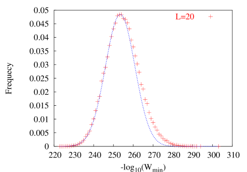
Figure 2: The frequency distribution of $-\log_{10}(W_{min})$ taking bin size $=1$ and starting with $10^{6}$ initial realizations for $L=20$. We fit the left tail of the data points with a Gaussian distribution with mean $\mu\approx 253.4$ and variance $\sigma^{2}\approx 55$.

As a check of our simulation algorithm, we calculated the probability of the minimum slope configurations for small $L$ and the numerical values match well with the values obtained from exact numerical calculation using the method in section.3. For example, the probability of the minimum slope, for $L=5$, is calculated to be $1.475\times 10^{-7}$ after averaging the data over $10^{6}$ realizations and the value is correct upto three significant digits. We have compared our results obtained from two procedures, i.e., the Monte Carlo simulation and exact numerical calculation and plotted negative of logarithm of the probabilities against $L$ in Fig.3 for $L\leq 12$.

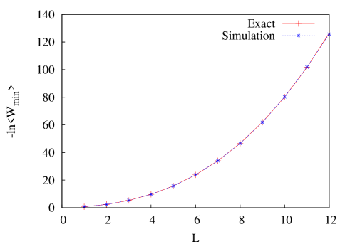
Figure 3: Exact numerical calculation and the Monte Carlo simulation for $L\leq 12$: Logarithm (base $e$) of the probability of the minimum slope configuration is plotted against the system size $L$ in the $1D$ Oslo ricepile model. The data is averaged over $10^{6}$ realizations.

For $h$ near $L$, $W(h)$ is a product of approximately $L^{3}$ different factors $F(t)$’s, the logarithm of $W(h)$ is a sum of $L^{3}$ random variables. While these variables $F(t)$’s are neither strictly independent nor they are identically distributed, our simulation suggest that correlations between these factors at different times are weak, so that we can expect central- limit-theorem like result to hold. Then $\log[W(h\simeq L)]$ may be expected to be normally distributed with a mean and variance both proportional to $L^{3}$ and $W(h)$ would be log-normally distributed. In fact, the experimentally obtained probability distribution function of $\log W$ shows significant deviations from gaussian [ Fig.2].

Assuming that the distribution of the random variable $X=-\ln[W(h\simeq L)]$ has the form $\frac{1}{\sqrt{2\pi\sigma^{2}}}\exp[-\frac{(X-\mu)^{2}}{2\sigma^{2}}]$, we get the probability of the minimum slope equal to

$$Prob_{L}(h_{1})=\langle W(h_{1})\rangle=\langle e^{-X}\rangle$$ (12)

Thus, if the gaussian approximation holds for the distribution,

$$\ln\langle W(h)\rangle\approx\langle\ln W(h)\rangle+\frac{\sigma^{2}}{2}$$ (13)

This estimate need not be precise as the terms contribute significantly to $\langle W(h\simeq L)\rangle$ are in the tail of the distributions and central limit theorem need not hold there.

However our numerical estimate indicates that this approximation is indeed very good. This is because the deviations from the gaussian behavior are stronger for smaller values of $W$, but these do not contribute much to $\langle W\rangle$. For example, from the simulation for $L=15$, we get $\mu\approx-270$, $\sigma^{2}\approx 95$, $\ln\langle W_{min}\rangle\approx-229$. The Gaussian approximation to distribution of $\ln W_{min}$ would give $\ln\langle W_{min}\rangle\approx-223$. In Fig.4, we have compared the actual values of $log_{10}\langle W_{min}\rangle$ from the simulation with the estimate from the Gaussian approximation for different values of the system size $L$.

In Fig.5 we have plotted negative of $\langle\log W_{min}\rangle$ as a function of $L$ and fitted it with a curve $ax^{3}+bx^{2}+cx$. We get a god fit for $a=0.0234\pm 0.0001$, $b=0.16\pm 0.05$ and $c=0.11\pm 0.2$.

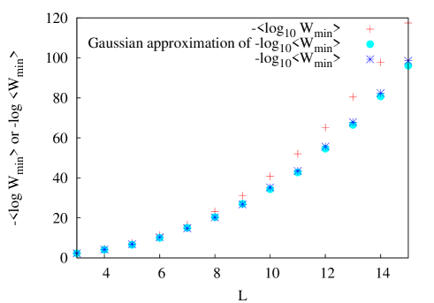
Figure 4: Comparision of $\langle W_{min}\rangle$, as computed directly from the simulations (blue $\star$), and as estimated by using the Gaussian approximation in Eq.13 (light blue bullet) for different system sizes $L$. Also shown is $-\langle\log_{10}W_{min}\rangle$ (red $+$).

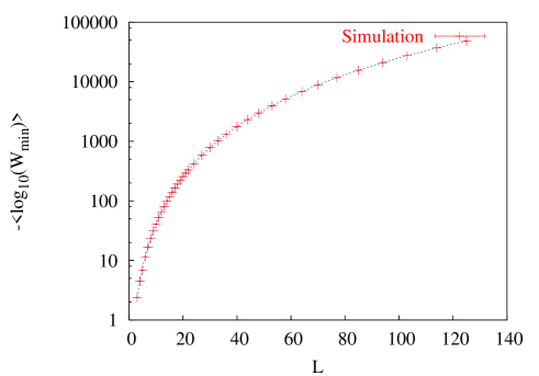
Figure 5: Monte Carlo estimate of $\langle\log W_{min}\rangle$ plotted against system size $L$ in the $1D$ Oslo ricepile model. The data points are fitted with $ax^{3}+bx^{2}+cx$ where $a=0.0234$, $b=0.16$ and $c=0.1$.

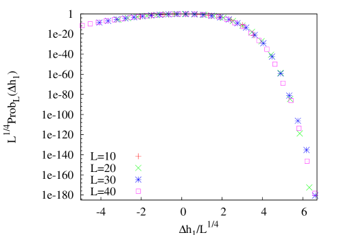
Figure 6: Scaling collapse for the probability distribution of height at site $1$ for systems of size $L=10,20,30,40$. $L^{1/4}Prob_{L}(\Delta h_{1})$ has been plotted against $(h_{1}-\bar{h}_{1})/L^{1/4}$. Each point is averaged over $10^{6}$ realizations.

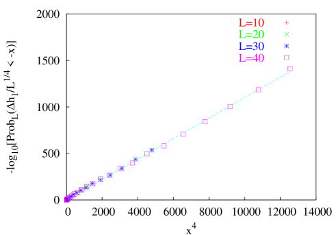
Figure 7: $log_{10}[Prob_{L}(\Delta h_{1}/L^{1/4}<-x)]$, for $x>0$, has been plotted against the scaling variable $x^{4}$ where $\Delta h_{1}=(h_{1}-\bar{h}_{1})$. The data points are fitted with a straight line $0.11x$ and it shows that the scaling function $g(-x)$ varies as $\exp(-\kappa x^{4})$ for $x\gg 1$.

Now we calculate the full probability distribution $Prob_{L}(h_{1})$ of height $h_{1}$ at site $1$. We take the average of this product over many realizations and estimate $\log[Prob_{L}(h_{1}\leq h)]$ using the Gaussian approximation. We thus determined $Prob_{L}(h_{1}=h)$ for different $h$, for $L=10,20,30,40$. The data is averaged over $10^{6}$ initial realizations. In Fig.6, we get a good scaling collapse by plotting $L^{\omega}Prob_{L}(h_{1}=h)$ against the scaling variable $(h_{1}-\bar{h}_{1})/L^{\omega}$ where $\omega\approx 1/4$. Therefore $Prob_{L}(h_{1}=h)$ a has scaling form $Prob_{L}(h_{1})=L^{-1/4}g[(h_{1}-\langle h_{1}\rangle)/L^{1/4}]$ at the central region as well as at the tail. We see from the scaling plot the scaling function is highly asymmetric about the origin.

Since the probability of minimum slope configurations varies as $\exp(-\kappa L^{3})$ for large $L$ and the height fluctuation $\Delta h_{1}=(h_{1}-\bar{h}_{1})$ scales with system sizes as $L^{1/4}$, the scaling function $g(x)$ must vary as $\exp(-\kappa x^{4})$. In Fig.7, we plot logarithm of $Prob_{L}(\Delta h_{1}/L^{1/4}<-x)$ versus $x^{4}$ for $x>0$ (i.e., fluctuations below average height). The data gives a reasonably good fit to a straight line with slope $0.11$.

V Summary

We have done a Monte Carlo simulation using importance sampling to study large deviations in the one dimensional Oslo ricepile model. We estimated probabilities of large height fluctuations of the pile and these probabilities are order $10^{-100}$ or even much less than this. We have shown that logarithm of the probability of large negative height fluctuation $\Delta h=-\alpha L$ varies as $-{\alpha}^{4}L^{3}$ for large $L$. We also calculated numerically the full probability distribution of height of the pile, and find that it has scaling form $L^{-1/4}g(\Delta h/L^{1/4})$, with $\log[g(x)]$ varying as $-x^{4}$ for large negative $x$.

VI Appendix

We illustate the procedure for generating the largest among $x(j,t)$’s, where $j\in{\bf u}$, using the algorithm given here. Consider independent random variables $x_{1}$, $x_{2}$, $x_{3}$, $x_{4}$, $x_{5}$ which are known to be uniformly distributed between the respective intervals as given below,

$\mbox{~{}~{}~{}~{}~{}~{}~{}~{}~{}~{}~{}~{}~{}~{}~{}~{}~{}~{}~{}~{}~{}}1.\mbox{~{}~{}}x_{1}\in[0,1]\\ \mbox{~{}~{}~{}~{}~{}~{}~{}~{}~{}~{}~{}~{}~{}~{}~{}~{}~{}~{}~{}~{}~{}}2.\mbox{~{}~{}}x_{2}\in[0,u]\\ \mbox{~{}~{}~{}~{}~{}~{}~{}~{}~{}~{}~{}~{}~{}~{}~{}~{}~{}~{}~{}~{}~{}}3.\mbox{~{}~{}}x_{3}\in[0,u]\\ \mbox{~{}~{}~{}~{}~{}~{}~{}~{}~{}~{}~{}~{}~{}~{}~{}~{}~{}~{}~{}~{}~{}}4.\mbox{~{}~{}}x_{4}\in[0,v]\\ \mbox{~{}~{}~{}~{}~{}~{}~{}~{}~{}~{}~{}~{}~{}~{}~{}~{}~{}~{}~{}~{}~{}}5.\mbox{~{}~{}}x_{5}\in[0,v]$

where we take $1\geq u\geq v$ without loss of generality. Then the cumulative probability distribution of $y$, the largest among these random numbers, is given by

$$Prob(y\leq x) = x,{\rm~{}for~{}}u\leq x\leq 1$$ (14)

$$= x^{3}/u^{2},{\rm~{}for~{}}v\leq x\leq u;$$

$$= x^{5}/(u^{2}v^{2}),{\rm~{}for~{}}0\leq x\leq v.$$

The distribution is drawn schematically in Fig. 8. To generate a variable $y$ with this distribution, we use the following algorithm: generate a number $z$ randomly between $0$ and $1$. Then following cases are possible.

1. If $u<z\leq 1$ we choose the largest random number to be $y=z$ and the maximum is surely $x_{5}$.
2. If $v^{3}/u^{2}<z\leq u$, we choose the largest random number to be $y=(zu^{2})^{1/3}$ and the maximum is chosen from $x_{3}$, $x_{4}$ and $x_{5}$ with probability $1/3$ each.
3. If $0\leq z\leq v^{3}/u^{2}$, we choose the largest random number to be $y=(zu^{2}v^{2})^{1/5}$ and the maximum is chosen from $x_{1}$, $x_{2}$, $x_{3}$, $x_{4}$ and $x_{5}$ with probability $1/5$ each.

If the resulting value of $y$ is less than $p$, the value is rejected, and the whole procedure is implemented afresh. Probability distributions for the maximum of more variables can be obtained similarly.

Figure 8: The probability $Prob(x_{max}<x)$ of $x_{max}$ being less than $x$ versus $x$.

References

- (1) O. E. Lanford, Entropy and equilibrium states in Classical Statistical Mechanics, Lecture Notes in Physics, Vol. 20, edited by A. Lenard (Springer, Berlin, 1973).
- (2) D. J. Evans and D. J. Searles, Advances in Physics, 51, 1529 (2002).
- (3) L. Bertini, A. De Sole, D. Gabrielli, G. Jona-Lasinio and C. Landim, Phys. Rev. Lett., 87, 040601 (2001).
- (4) B. Derrida and J. L. Lebowitz, Phys. Rev. Letts., 80, 209 (1998).
- (5) M. Depken and R. Stinchcombe, Phys. Rev. Letts., 93, 040602 (2004). M. Depken and R. Stinchcombe, Phys. Rev. E, 71, 036120 (2005).
- (6) C. Giardina, J. Kurchan and L. Peliti, cond-mat/0511248.
- (7) P. Pradhan and D. Dhar, Phys Rev. E, 73, 021303 (2006).
- (8) P. Grassberger, Comp. Phys. Comm. 147, 64 (2002) [ cond-mat/0201313].
- (9) G. Pruessner, Phys. Rev. E, 67, 030301(R) (2003).
- (10) K. Christensen, A. Corral, V. Frette, J. Feder, and T. Jssang, Phys. Rev. Lett., 77, 107 (1996).
- (11) V. Frette, Phys. Rev. Lett. 70, 2762 (1993).
- (12) D. Dhar, Physica A, 340, 535 (2004).
- (13) A. Chua and K. Christensen, cond-mat/0203260.
- (14) D. Dhar and P. Pradhan, JSTAT, online at stacks.iop.org/JSTAT/1742-5468/2004/P05002.
- (15) This time can be reduced to if we store the weights of configurations to collect terms together.
- (16) This is similar to the Monte Carlo in equilibrium statistical physics, where thermodynamic quantities like free enrgy can be estimated well, but not the partition function.