Fermi surface renormalization and confinement in two coupled metallic chains

Abstract

Using a non-perturbative functional renormalization group approach involving both fermionic and bosonic fields we calculate the interaction-induced change of the Fermi surface of spinless fermions moving on two chains connected by weak interchain hopping $t_{\bot}$. For a model containing interband backward scattering only we show that the distance $\Delta$ between the Fermi momenta associated with the bonding and the antibonding band can be strongly reduced, corresponding to a large reduction of the effective interchain hopping $t_{\bot}^{\ast}\propto\Delta$. A self-consistent one-loop approximation neglecting marginal vertex corrections and wave-function renormalizations predicts a confinement transition for sufficiently large interchain backscattering, where the renormalized $t_{\bot}^{\ast}$ vanishes. However, a more accurate calculation taking vertex corrections and wave-function renormalizations into account predicts only weak confinement in the sense that $0<|t_{\bot}^{\ast}|\ll|t_{\bot}|$. Our method can be applied to other strong-coupling problems where the dominant scattering channel is known.

I Introduction

In strongly correlated Fermi systems electron-electron interactions can have drastic effects on the geometry and the topology of the Fermi surface. For example, strong forward scattering can give rise to a Pomeranchuk instability, where the shape of the Fermi surface spontaneously changes such that it has a lower symmetry than the underlying lattice Pomenanchuk58 . Another example is the Lifshitz transition Lifshitz60 , where the topology of the Fermi surface changes discontinuously without symmetry breaking as a function of some external control parameter. This gives rise to anomalies in thermodynamic and kinetic properties of a metal. Conditions on the range and the strength of the interaction leading to Pomeranchuk and Lifshitz transitions have recently been derived in Ref. [Quintanilla06, ].

In this work we shall focus on another type of phase transition associated with the geometry of the Fermi surface, which we call confinement transition. This quantum phase transition can occur in quasi one-dimensional metals with an open Fermi surface, consisting of two disconnected weakly curved sheets. Due to strong interactions, the curvature of the Fermi sheets can be smoothed out and can eventually vanish in certain sectors. In the extreme case, the renormalized Fermi surface consists of two completely flat parallel planes. The motion of the fermions in real space is then strictly one-dimensional, although in the absence of interactions it is not. We therefore call such a transition confinement transition. In the confined state the low-energy properties of the system resemble that of a one-dimensional Luttinger liquid. Because the Fermi surface in the confined state has an additional nesting symmetry, at the confinement transition the symmetry of the Fermi surface increases, in contrast to the Pomeranchuk instability, where interactions lower the symmetry of the Fermi surface. An interaction-induced flattening of the Fermi surface might also play a role in the Hubbard model close to half filling, where the bare Fermi surface consists of four almost flat sectors. Completely flat parts of the Fermi surface can give rise to non-Fermi liquid behavior Luther94 ; Zheleznyak97 ; Ferraz03 . Evidence of an interaction-induced flattening of the Fermi surface of the Hubbard model close to half filling has been found in Ref. [Honerkamp01, ].

Similar to the Pomeranchuk transition, the confinement transition is a strong-coupling phenomenon. Hence, the usual weak coupling perturbative expansions are not sufficient to study this transition. Due to a lack of controlled methods to deal with strongly interacting fermions in dimensions larger than one, it is very difficult to study the confinement transition. To shed some light on the underlying mechanism, we shall in this work consider the simpler problem of just two metallic spinless chains coupled by weak interchain hopping $t_{\bot}$. The confined state corresponds to a vanishing renormalized interchain hopping $t_{\bot}^{\ast}=0$, so that electrons cannot move from one chain to the other, in spite of the fact that the bare interchain hopping is finite. In a subsequent paper Ledowski06 , we shall discuss the more difficult confinement problem in an infinite array of coupled chains. It turns out that the basic mechanism responsible for the tendency towards confinement can already be understood from the simpler two-chain problem.

Because perturbation theory in the two-chain problem is plagued by the usual infrared divergencies of one-dimensional Fermi systems, even in the limit of weak interactions the Fermi surface cannot be calculated within renormalized perturbation theoryNeumayr03 ; Dusuel03 . In dimensions $D\geq 2$ the Fermi surface deformation has been studied to all orders in perturbation theory in Ref. [Feldman96, ] for a general class of models. Within the framework of the renormalization group (RG) the Fermi surface can be defined non-perturbatively from the requirement that the relevant coupling constants $r_{l}({\bm{k}}_{F})$ related to the self-energy $\Sigma({\bm{k}}_{F},\omega=0)$ at the true Fermi surface ${\bm{k}}_{F}$ flow into a fixed point of the RG Kopietz01 ; Ledowski03 . In Ref. [Ledowski05, ] we have calculated the shift of the Fermi surface in the two-chain system within the usual weak coupling expansion of the RG $\beta$-functions. We have shown that interchain backscattering gives rise to the dominant logarithmic renormalization of the distance $\Delta=k^{+}-k^{-}$ between the Fermi momenta $k^{+}$ and $k^{-}$ associated with the bonding and the antibonding band. Denoting by $\Delta_{1}$ the value of $\Delta$ within the Hartree-Fock approximation, the self-consistency condition for the true Fermi point distance in the spinless two-chain system can be cast into the form

$$\Delta=\frac{\Delta_{1}}{1+2g_{0}^{2}\ln(\Lambda_{0}/\Delta)}\;,$$ (1)

where $\Lambda_{0}$ is an ultraviolet cutoff and $g_{0}$ is the bare value of the dimensionless coupling constant describing interchain backscattering, which will be defined more precisely in Sec. IV.2. From Eq. (1) we see that sufficiently large interchain backscattering strongly reduces the value of $\Delta$. But the renormalized $\Delta$ never vanishes, so that there is no true confinement transition. One should keep in mind, however, that Eq. (1) has been derived by expanding the RG $\beta$-functions to second order in the coupling constants, so that it is not allowed to extrapolate this expression to large values of $g_{0}$.

To find out whether in the spinless two-chain system sufficiently strong interchain-backscattering can give rise to a confinement transition where the renormalized effective interchain hopping $t_{\bot}^{\ast}\propto k^{+}-k^{-}$ vanishes, we use here a generalization of the collective field functional RG approach with momentum transfer cutoff developed in Ref. [Schuetz05, ]. It turns out that with this approach we can analyze the regime where the dimensionless interchain backscattering interaction $g_{0}$ is of the order of unity. The crucial point is that from the weak coupling analysis Ledowski05 we know that the confinement transition is driven by interchain backscattering, so that it is natural to decouple the interaction in this scattering channel via a suitable bosonic Hubbard-Stratonovich field. Simple truncations in the resulting mixed boson-fermion theory correspond to infinite resummations in an expansion of the RG $\beta$-functions in powers of $g_{0}$.

II Effective low-energy model

We consider spinless fermions confined to two chains that are coupled by weak interchain hopping $t_{\bot}$. The kinetic energy of the two-chain system is diagonalized by forming symmetric (bonding band) and antisymmetric (antibonding band) combinations of the eigenstates associated with isolated chains. Denoting by $\epsilon_{k}$ the energy dispersion of a single chain in the absence of interchain hopping, the energy dispersion of the non-interacting system is $\epsilon_{k}^{\sigma}=\epsilon_{k}-\sigma t_{\bot}$, where $\sigma=+1$ labels the bonding band and $\sigma=-1$ labels the antibonding band. It is useful to think of $\sigma$ as a pseudospin label Fabrizio93 , in which case $t_{\bot}=h$ corresponds to a uniform magnetic field $h$ in the $z$-direction.

The problem of finding the low-energy properties of two coupled metallic chains has been studied previously by many authors Dusuel03 ; Ledowski05 ; Fabrizio93 ; Brazovskii85 ; Bourbonnais91 ; Kusmartsev92 ; Finkelstein93 ; Boies95 ; Balents96 ; Arrigoni98 ; Ledermann00 ; Louis01 ; Caron02 ; Bourbonnais04 ; Nickel06 ; Tsuchiizu06 . However, the problem of self-consistently calculating the true Fermi surface has only recently been addressed Dusuel03 ; Ledowski05 ; Louis01 . At low energies all possible scattering processes in the spinless two-chain system can be divided into four different classes Fabrizio93 : (1) forward scattering processes, parameterized in terms of three different coupling constants $f^{++}$, $f^{--}$ and $f^{+-}=f^{-+}$, where the labels indicate the band of the fermions involved in the scattering process; (2) interband backward scattering, which in pseudospin language corresponds to transverse spin-exchange, so that we shall call the corresponding dimensionful coupling constant $J^{\bot}$ (the associated dimensionless coupling $g_{0}$ will be introduced in Sec. IV.2); (3) pair-tunneling, which can also be viewed as interband Umklapp scattering, parameterized in terms of a coupling constant by $u$; and finally (4) intraband Umklapp scattering, which is expected to be important only at commensurate fillings. Neglecting the latter process and setting for simplicity $f^{++}=f^{--}$, the low-energy interactions can be expressed in terms of four marginal coupling constants $f=\frac{1}{2}(f^{+-}+f^{++})$, $J^{\parallel}=\frac{1}{2}(f^{+-}-f^{++})$, $J^{\bot}$, and $u$. In the bonding-antibonding basis the system can then be modeled by the following effective Euclidean action in pseudospin notation,

$$S[\bar{\psi},\psi] = \sum_{\sigma}\int_{K}(-i\omega+\xi_{k}^{\sigma})\bar{\psi}_{K}^{\sigma}\psi_{K}^{\sigma}$$

$$+\frac{1}{2}\int_{\bar{K}}\left[f(\bar{k})\bar{\rho}_{\bar{K}}\rho_{\bar{K}}-J^{\parallel}(\bar{k})\bar{m}_{\bar{K}}m_{\bar{K}}\right]$$

$$+\int_{\bar{K}}\left[u(\bar{k})\left(\bar{s}_{\bar{K}}\bar{s}_{-\bar{K}}+s_{\bar{K}}s_{-\bar{K}}\right)-2J^{\bot}(\bar{k})\bar{s}_{\bar{K}}s_{\bar{K}}\right]\;,$$

where $\xi_{k}^{\sigma}=\epsilon_{k}-\mu-\sigma h$, and we have introduced the following composite fields,

$$\rho_{\bar{K}} = \sum_{\sigma}\int_{K}\bar{\psi}_{K}^{\sigma}\psi_{K+\bar{K}}^{\sigma}\;,$$ (3a)

$$m_{\bar{K}} = \sum_{\sigma}\sigma\int_{K}\bar{\psi}_{K}^{\sigma}\psi_{K+\bar{K}}^{\sigma}\;,$$ (3b)

$$s_{\bar{K}} = \int_{{K}}\bar{\psi}_{K}^{-}\psi_{K+\bar{K}}^{+}\;.$$ (3c)

We use the imaginary time formalism at zero temperature and have introduced collective labels $K=(k,i\omega)$ for fermionic fields and $\bar{K}=(\bar{k},i\bar{\omega})$ for bosonic fields, with the notation $\int_{K}=\int\frac{dkd\omega}{(2\pi)^{2}}$. Note that the Fourier components of the density and the longitudinal spin-density field satisfy $\rho_{-K}=\rho_{K}$ and $m_{-K}=m_{K}$, while the spin-flip field $s_{K}$ is complex and do not have this symmetry. The interaction functions $f(\bar{k})$, $J^{\parallel}(\bar{k})$, $J^{\bot}(\bar{k})$, and $u(\bar{k})$ should be considered as phenomenological low-energy couplings which are only non-zero for $|\bar{k}|\leq\Lambda_{0}\ll k_{F}$. Hence, these couplings should not be directly compared with the bare coupling constant in the Hubbard model footnotehubbard . The signs and normalizations in Eq. (LABEL:eq:action1) are chosen such that for $J^{\bot}=J^{\parallel}$ the model has rotational invariance in pseudo-spin space, and that for the Hubbard model all couplings are positive footnotehubbard . However, in our effective low energy model there is no reason to expect rotational invariance in pseudospin-space, so that in general $J^{\parallel}(\bar{k})\neq J^{\bot}(\bar{k})$.

The model defined in (LABEL:eq:action1) is still quite complicated and contains many interaction processes which are not essential for the confinement transition. In fact, from our previous weak coupling analysis Ledowski05 we know that the dominant renormalization of the difference between the Fermi points is due to the interchain backscattering process described by the coupling $J^{\bot}(\bar{k})$. In this work we study a minimal model describing the confinement transition by simply neglecting the forward scattering interactions $f(\bar{k})$ and $J^{\parallel}(\bar{k})$, as well as the pair tunneling coupling $u(\bar{k})$ in Eq. (LABEL:eq:action1). However it is known Brazovskii85 ; Boies95 that sufficiently strong pair tunneling can destabilize the Luttinger liquid phase; we shall come back to this point in Sec. V. In pseudospin language, our model then describes a one-dimensional spin $S=1/2$ Fermi system subject to a uniform magnetic field in $z$-direction with an attractive ferromagnetic spin exchange involving only the transverse ($xy$) spin components. The latter tends to align the spins in the direction perpendicular to the magnetic field. The Fermi surface renormalization is essentially determined by the competition between the $xy$-exchange interaction and the external constraint imposed by the uniform magnetic field, which tends to align the spins along the $z$-axis. The phase diagram of the model (LABEL:eq:action1) in the space of all couplings has been discussed by Fabrizio Fabrizio93 . The qualitative behavior of the weak coupling RG flow in the space of couplings spanned by $J^{\parallel}$, $J^{\bot}$ and $u$ is shown in Fig. 1.

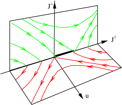
Figure 1: (Color Online) Qualitative behavior of the weak coupling RG flow of the model (LABEL:eq:action1) in the space of coupling constants $J^{\parallel}$, $J^{\bot}$ and $u$. The thick black line is the line of fixed points describing the stable Luttinger liquid phase.

Obviously, there is a finite regime in coupling space where the spinless two-chain system is a stable Luttinger liquid, with gapless excitations. In this work we shall assume that the qualitative fixed point structure suggested by the weak coupling analysis remains correct even in the strong coupling regime. We can therefore choose the bare parameters such that the system belongs to the basin of attraction of the Luttinger liquid fixed point manifold.

At low energies we may further simplify our model (at least in the deconfined phase) by linearizing the energy dispersion at the Fermi surface, which for our model consists of four points $\alpha k^{\sigma}$, where the chirality index $\alpha=\pm 1$ labels the left/right Fermi point. Note that the true Fermi points are defined via

$$\epsilon_{\alpha{k}^{\sigma}}-\mu-\sigma h+\Sigma^{\sigma}(\alpha k^{\sigma},i0)=0\;,$$ (4)

where $\Sigma^{\sigma}(\alpha k^{\sigma},i0)$ is the exact self-energy for vanishing frequency and for momenta at the true Fermi surface $\alpha k^{\sigma}$ of the interacting system. To linearize the energy dispersion at the true Fermi surface, we add and subtract from the non-interacting energy dispersion the counter-term

$$\mu^{\sigma}_{0}=-\Sigma^{\sigma}(\alpha k^{\sigma},i0)\;,$$ (5)

and approximate

$$\xi_{\alpha k^{\sigma}+k}^{\sigma} = \epsilon_{\alpha k^{\sigma}+k}-\mu-\sigma h$$ (6)

$$=\epsilon_{\alpha k^{\sigma}+k}-\mu-\sigma h+\Sigma^{\sigma}(\alpha k^{\sigma},i0)-\Sigma^{\sigma}(\alpha k^{\sigma},i0)$$

$$\approx\alpha v^{\sigma}_{0}k+\mu^{\sigma}_{0}\;,$$

where $v_{0}^{\sigma}$ is the bare Fermi velocity at the true Fermi surface for pseudospin $\sigma$. In analogy with the definition of the couplings in the Tomonaga-Luttinger model Solyom79 , we now generalize the interaction by introducing chirality indices $J^{\bot}\rightarrow J^{\bot}_{\alpha\alpha^{\prime}}$. We shall refer to the diagonal processes $J^{\bot}_{\alpha\alpha}$ as chiral interactions (these are called $g_{4}$ processes in the Tomonaga-Luttinger model). Similarly, off-diagonal elements $J^{\bot}_{\alpha,-{\alpha}}$ will be called non-chiral processes (corresponding to the $g_{2}$-processes in the Tomonaga-Luttinger model). Defining new fields

$$\psi^{\sigma}_{K\alpha}=\psi_{\alpha k^{\sigma}+k,i\omega}^{\sigma}\;,$$ (7)

we replace the action (LABEL:eq:action1) by the following effective low-energy action describing the physics of the confinement transition in our system of two spinless metallic chains,

$$S[\bar{\psi},\psi] = \sum_{\sigma,\alpha}\int_{K}(-i\omega+\alpha v^{\sigma}_{0}k+\mu^{\sigma}_{0})\bar{\psi}^{\sigma}_{K\alpha}\psi^{\sigma}_{K\alpha}$$ (8)

$$- 2\sum_{\alpha\alpha^{\prime}}\int_{\bar{K}}J^{\bot}_{\alpha\alpha^{\prime}}\bar{s}_{\bar{K}\alpha}s_{\bar{K}\alpha^{\prime}}\;,$$

where it is understood that the $\bar{k}$-integration has a momentum transfer cutoff $|\bar{k}|\leq\Lambda_{0}\ll k_{F}$, and

$$s_{\bar{K}\alpha} = \int_{K}\bar{\psi}^{-}_{K\alpha}\psi^{+}_{K+\bar{K}\alpha}\;.$$ (9)

III Exact RG flow equations

III.1 Hubbard Stratonovich transformation

Because the confinement transition is a strong coupling phenomenon, the usual weak coupling RG approach based on the expansion in powers of $J^{\bot}_{\alpha\alpha^{\prime}}$ is not suitable. To develop a RG approach which does not rely on a weak coupling expansion, we decouple the spin-flip interaction with the help of a complex Hubbard-Stratonovich field $\chi_{\alpha}$. For convenience we collect all fields in a super-field,

$$\Phi=(\psi_{\alpha}^{+},\bar{\psi}_{\alpha}^{+},\psi_{\alpha}^{-},\bar{\psi}_{\alpha}^{-},\chi_{\alpha},\bar{\chi}_{\alpha})\;.$$ (10)

Taking into account that there are two chiralities $\alpha=\pm 1$, our super-field has totally 12 components (8 fermionic and 4 bosonic ones). The ratio of the partition functions with and without interactions can then be written as

$$\frac{\cal{Z}}{{\cal{Z}}_{0}}=\frac{\int{\cal{D}}[\Phi]e^{-S_{0}[\Phi]-S_{1}[\Phi]}}{\int{\cal{D}}[\Phi]e^{-S_{0}[\Phi]}}\;,$$ (11)

with the Gaussian part of the effective action given by

$$S_{0}[\Phi] = \sum_{\sigma,\alpha}\int_{K}(-i\omega+\alpha v^{\sigma}_{0}k+\mu^{\sigma}_{0})\bar{\psi}^{\sigma}_{K\alpha}\psi^{\sigma}_{K\alpha}$$ (12)

$$+ \frac{1}{2}\sum_{\alpha\alpha^{\prime}}\int_{\bar{K}}[{\bf{J}}^{\bot}]^{-1}_{\alpha\alpha^{\prime}}\bar{\chi}_{\bar{K}\alpha}\chi_{\bar{K}\alpha^{\prime}}\;.$$

Here ${\bf{J}}^{\bot}$ is a matrix in chirality space with matrix elements given by ${J}^{\bot}_{\alpha\alpha^{\prime}}$, and the interaction is

$$S_{1}[\Phi] = \sum_{\alpha}\int_{\bar{K}}\bigl{[}\bar{s}_{\bar{K}\alpha}\chi_{\bar{K}\alpha}+s_{\bar{K}\alpha}\bar{\chi}_{\bar{K}\alpha}\bigr{]}\;.$$ (13)

A graphical representation of the bare interaction vertices in Eq. (13) is shown in Fig. 2.

Figure 2: Bare interaction vertices of the action $S_{1}[\Phi]$ given in Eq. (13). The fermionic fields $\psi^{\sigma}$ and $\bar{\psi}^{\sigma}$ are denoted by solid arrows, with the spin-projection $\sigma=\pm 1$ written next to the arrows. Bosonic spin-flip fields $\chi$ and $\bar{\chi}$ are denoted by wavy arrows. Incoming arrows denote $\psi^{\sigma}$ and $\chi$, while outgoing arrows correspond to the conjugate fields $\bar{\psi}^{\sigma}$ and $\bar{\chi}$.

The coupled RG flow equations for the one-line irreducible vertices of the above mixed boson-fermion theory can be obtained as a special case of the general flow equations given in Ref. [Schuetz05, ].

III.2 Functional RG flow equations in momentum transfer cutoff scheme

In order to calculate the true Fermi surface, we need to know the exact counter-term $\mu^{\sigma}_{0}=-\Sigma(\alpha k^{\sigma},i0)$, which can be obtained from the flowing self-energy $\Sigma_{\Lambda}^{\sigma}(K,\alpha)$ in the limit of vanishing infrared cutoff $\Lambda\rightarrow 0$. The form of the flow equation for $\Sigma_{\Lambda}^{\sigma}(K,\alpha)$ depends on the RG method employed. Here we use the hierarchy of functional RG equations for the one-line irreducible vertices Wetterich93 ; Morris94 of mixed boson-fermion models developed in Ref. [Schuetz05, ]. A similar approach involving both fermionic and bosonic fields has been developed in Refs. [Wetterich02, ; Baier04, ]. In principle, one can also obtain the flowing self-energy within the purely fermionic parameterization of the hierarchy of flow equations Kopietz01 ; Ledowski05 ; Salmhofer01 . However, with the usual truncations necessary in this approach it is not possible to reach the strong coupling regime.

In the momentum transfer cutoff scheme Schuetz05 we impose a cutoff $\Lambda$ only on the momentum $\bar{k}$ transfered by the collective bosonic field. The resulting RG flow equation for the fermionic self-energy $\Sigma_{\Lambda}^{\sigma}(K,\alpha)$ is shown graphically in Fig. 3.

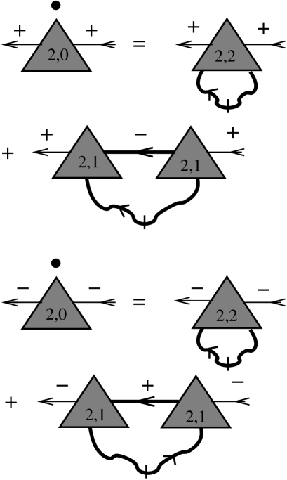
Figure 3: Exact flow equation for the fermionic self-energy $\Sigma^{\sigma}_{\Lambda}(K,\alpha)$ in the momentum transfer cutoff scheme. The thick solid arrow is the flowing fermionic Green function and the thick wavy line with a slash is the flowing single scale spin-flip propagator defined in Eq. (17). The one-line irreducible vertices are represented by shaded triangles. A label $(n,m)$ inside a shaded triangle means that the vertex has $n$ fermionic and $m$ bosonic external legs.

The corresponding analytic expression is

$$\partial_{\Lambda}\Sigma^{\sigma}_{\Lambda}(K,\alpha)$$ (14)

$$=\int_{\bar{K}}\dot{F}^{\sigma\bar{\sigma}}_{\Lambda}(\bar{K},\alpha)\Gamma^{(2,2)}_{\Lambda}(K\sigma,-K\sigma;\bar{K},-\bar{K},\alpha)$$

$$+\int_{\bar{K}}\dot{F}^{\sigma\bar{\sigma}}_{\Lambda}(\bar{K},\alpha)G^{\bar{\sigma}}_{\Lambda}(K+\bar{K}+\alpha\sigma\Delta,\alpha)$$

$$\times\Gamma^{(2,1)}_{\Lambda}(K\sigma;K+\bar{K},\bar{\sigma};-\bar{K},\alpha)$$

$$\times\Gamma^{(2,1)}_{\Lambda}(K+\bar{K},\bar{\sigma};K,\sigma;\bar{K},\alpha)\;.$$

Here $G_{\Lambda}^{\sigma}(K,\alpha)$ is the flowing fermionic single-particle Green function for a given pseudospin $\sigma$ and chirality index $\alpha$. We use the notation $\bar{\sigma}=-\sigma$ and measure the wave-vectors $k$ with respect to the true Fermi momenta $\alpha k^{\sigma}$, defining

$$G_{\Lambda}^{\sigma}(K,\alpha)=G_{\Lambda}^{\sigma}(\alpha k^{\sigma}+k,i\omega)\;,$$ (15)

and

$$G^{\bar{\sigma}}_{\Lambda}(K+\alpha\sigma\Delta,\alpha)=G^{\bar{\sigma}}_{\Lambda}(\alpha k^{\bar{\sigma}}+k+\alpha\sigma\Delta,i\omega)\;.$$ (16)

The shift $\alpha\sigma\Delta=\alpha\sigma(k^{+}-k^{-})$ in the argument of $G_{\Lambda}^{\bar{\sigma}}$ in Eq. (14) is due to the fact that in $G_{\Lambda}^{\bar{\sigma}}(K,\alpha)$ the wave-vector $k$ is measured with respect to a different reference point than in $G_{\Lambda}^{{\sigma}}(K,\alpha)$. The function $\dot{F}^{\sigma\bar{\sigma}}_{\Lambda}(\bar{K}\alpha)$ in Eq. (14) is the single scale bosonic spin-flip propagator, which is defined by

$$\dot{F}^{\sigma\bar{\sigma}}_{\Lambda}(\bar{K}\alpha)=-\delta(|\bar{k}|-\Lambda)[{\bf{F}}^{\sigma\bar{\sigma}}_{\Lambda}(\bar{K})]_{\alpha\alpha}\;,$$ (17)

where ${\bf{F}}^{\sigma\bar{\sigma}}_{\Lambda}(\bar{K})$ is a matrix in chirality space whose inverse has the matrix elements

$$[{\bf{F}}^{\sigma\bar{\sigma}}_{\Lambda}(\bar{K})]^{-1}_{\alpha\alpha^{\prime}}=[2{\bf{J}}^{\bot}]^{-1}_{\alpha\alpha^{\prime}}-\delta_{\alpha\alpha^{\prime}}\Pi_{\Lambda}^{\sigma\bar{\sigma}}(\bar{K},\alpha)\;,$$ (18)

where $\Pi_{\Lambda}^{\sigma\bar{\sigma}}(\bar{K},\alpha)$ is the flowing spin-flip susceptibility. In the momentum transfer cutoff scheme, the RG flow of $\Pi_{\Lambda}^{\sigma\bar{\sigma}}(\bar{K},\alpha)$ is driven by the one-line irreducible vertex with four external boson legs, as shown in Fig. 4.

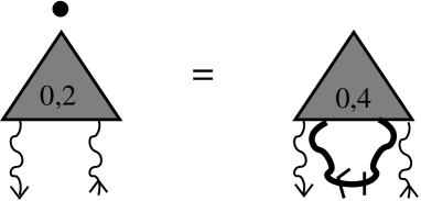
Figure 4: Exact flow equation for the spin-flip susceptibility in the momentum transfer cutoff scheme.

The vertices $\Gamma^{(2,1)}_{\Lambda}(K\sigma;K^{\prime}\bar{\sigma};\bar{K},\alpha)$ in Eq. (14) are the flowing spin-flip vertices with two fermionic and one bosonic external legs. In the momentum transfer cutoff scheme these vertices satisfy the exact flow equations shown in graphically in Fig. 5, with initial condition

$$\Gamma^{(2,1)}_{\Lambda_{0}}(K\sigma;K^{\prime}\bar{\sigma};\bar{K},\alpha)=1\;.$$ (19)

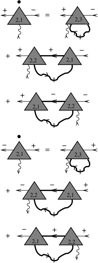
Figure 5: Exact flow equation for the spin-flip vertices in the momentum transfer cutoff scheme.

Finally, the vertex $\Gamma^{(2,2)}_{\Lambda}$ on the right-hand side of Eq. (14) is the one-line irreducible vertex with two fermionic and two bosonic external legs. We do not give the flow equation for this vertex, because purely bosonic vertices with more than two external legs and mixed vertices with two fermionic and more than one bosonic external leg have negative scaling dimensions and are irrelevant Schuetz05 . We expect that their effect can be implicitly taken into account by re-defining the numerical values of the relevant and marginal couplings Polchinski84 .

The initial condition for the fermionic self-energy at scale $\Lambda=\Lambda_{0}$ is simply

$$\Sigma^{\sigma}_{\Lambda_{0}}(K,\alpha)=0\;.$$ (20)

Similarly, the vertices with two fermion legs and more than one boson leg appearing on the right-hand side of the flow equation for the spin-flip vertex shown in Fig. 5 also vanish at the initial scale. However, the price we pay for introducing a cutoff only in the momentum transfer are non-trivial initial conditions for the purely bosonic vertices, which are initially given by closed fermion loops Schuetz05 . In particular, the loop with two external boson legs is initially given by the non-interacting spin-flip susceptibility,

$$\Pi^{\sigma\bar{\sigma}}_{\Lambda_{0}}(\bar{K},\alpha) = -\int_{K}G_{\Lambda_{0}}^{\sigma}(K,\alpha)G_{\Lambda_{0}}^{\bar{\sigma}}(K+\bar{K}+\alpha\sigma\Delta,\alpha)\;,$$

where for our model with linear energy dispersion,

$$G_{\Lambda_{0}}^{\sigma}(K,\alpha)=\frac{1}{i\omega-\alpha v^{\sigma}_{0}k-\mu^{\sigma}_{0}}\;.$$ (22)

Denoting by

$$\Delta_{0}=k^{+}_{0}-k^{-}_{0}$$ (23)

the distance between the Fermi momenta $k_{0}^{+}$ and $k_{0}^{-}$ in the absence of interactions, the relation between the true distance $\Delta=k^{+}-k^{-}$ and $\Delta_{0}$ can be expressed in terms of the counter-terms $\mu^{\sigma}_{0}=-\Sigma(\alpha k^{\sigma},i0,\alpha)$ as follows,

$$\Delta=\Delta_{0}+\left[\frac{\mu^{+}_{0}}{v^{+}_{0}}-\frac{\mu^{-}_{0}}{v^{-}_{0}}\right]\;,$$ (24)

see also Eq. (50) below. Using Eqs. (22) and (24) we can explicitly evaluate Eq. (LABEL:eq:Piinitial),

$$\Pi^{\sigma\bar{\sigma}}_{\Lambda_{0}}(\bar{K},\alpha) = \frac{1}{2\pi v^{\sigma}_{0}}\frac{v^{\bar{\sigma}}_{0}(\sigma\Delta_{0}+\alpha\bar{k})}{v^{\bar{\sigma}}_{0}(\sigma\Delta_{0}+\alpha\bar{k})-i\bar{\omega}}\;.$$ (25)

III.3 Rescaled flow equations and classification of vertices

To classify the various vertices according to their relevance, it is useful to make them dimensionless by multiplying them with a suitable power of the running cutoff $\Lambda$. Following Ref. [Schuetz05, ], we define dimensionless fermionic labels $Q=(q,i\epsilon)=(k/\Lambda,i\omega/\Omega_{\Lambda})$, and bosonic ones $\bar{Q}=(\bar{q},i\bar{\epsilon})=(\bar{k}/\Lambda,i\bar{\omega}/\Omega_{\Lambda})$. Here $\Omega_{\Lambda}=v_{F}\Lambda$, where $v_{F}$ is some average Fermi velocity. For simplicity we shall write the above relations as $Q=K/\Lambda$ and $\bar{Q}=\bar{K}/\Lambda$. We consider all rescaled quantities as functions of the logarithmic flow parameter $l=\ln(\Lambda_{0}/\Lambda)$.

In order to define the Fermi surface within the framework of the RG, we subtract the counter-term $\Sigma^{\sigma}(\alpha k^{\sigma},i0,\alpha)=-\mu^{\sigma}_{0}$ from the flowing self-energy and then rescale Kopietz01 ,

$$\tilde{\Sigma}_{l}^{\sigma}(Q,\alpha) = \frac{Z^{\sigma}_{l}}{\Omega_{\Lambda}}\left[\Sigma_{\Lambda}^{\sigma}(K,\alpha)-\Sigma^{\sigma}(\alpha k^{\sigma},i0)\right]$$ (26)

$$= \frac{Z^{\sigma}_{l}}{\Omega_{\Lambda}}\left[\Sigma_{\Lambda}^{\sigma}(\Lambda Q,\alpha)+\mu^{\sigma}_{0}\right]\;.$$

Here $Z^{\sigma}_{l}$ is the flowing wave-function renormalization factor, which is defined in terms of the flowing self-energy as follows,

$$Z^{\sigma}_{l}=1+\left.\frac{\partial\tilde{\Sigma}_{l}^{\sigma}(0,i\epsilon,\alpha)}{\partial(i\epsilon)}\right|_{\epsilon=0}\;.$$ (27)

The corresponding rescaled fermionic propagator is

$$\tilde{G}_{l}^{\sigma}(Q,\alpha)=\frac{\Omega_{\Lambda}}{Z^{\sigma}_{l}}G^{\sigma}_{\Lambda}(\Lambda Q,\alpha)\;.$$ (28)

The rescaled self-energy satisfies the exact RG flow equationKopietz01 ; Ledowski03

$$\partial_{l}\tilde{\Sigma}_{l}^{\sigma}(Q,\alpha)=(1-\eta^{\sigma}_{l}-q\partial_{q}-\epsilon\partial_{\epsilon})\tilde{\Sigma}_{l}^{\sigma}(Q,\alpha)+\dot{{\Gamma}}_{l}^{\sigma}(Q,\alpha)\;,$$ (29)

where the flowing anomalous dimension of the Fermi fields is

$$\eta_{l}^{\sigma}=-\partial_{l}\ln Z^{\sigma}_{l}=\left.-\frac{\partial\dot{{\Gamma}}^{\sigma}_{l}(0,i\epsilon,\alpha)}{\partial(i\epsilon)}\right|_{\epsilon=0}\;,$$ (30)

and the function $\dot{{\Gamma}}_{l}^{\sigma}(Q,\alpha)$ follows from Eq. (14),

$$\dot{{\Gamma}}_{l}^{\sigma}(Q,\alpha) = \frac{Z^{\sigma}_{l}}{\Omega_{\Lambda}}[-\Lambda\partial_{\Lambda}\Sigma_{\Lambda}^{\sigma}(K,\alpha)]$$ (31)

$$= \int_{\bar{Q}}\dot{\tilde{F}}^{\sigma\bar{\sigma}}_{l}(\bar{Q},\alpha)\tilde{\Gamma}^{(2,2)}_{l}(Q,\sigma;-Q\sigma;\bar{Q},-\bar{Q},\alpha)$$

$$+ \int_{\bar{Q}}\dot{\tilde{F}}^{\sigma\bar{\sigma}}_{l}(\bar{Q},\alpha)\tilde{G}^{\bar{\sigma}}_{l}(Q+\bar{Q}+\alpha\sigma\tilde{\Delta}_{l}^{\ast},\alpha)$$

$$\times\tilde{\Gamma}^{(2,1)}_{l}(Q,\sigma;Q+\bar{Q},\bar{\sigma};-\bar{Q},\alpha)$$

$$\times\tilde{\Gamma}^{(2,1)}_{l}(Q+\bar{Q},\bar{\sigma};Q\sigma;\bar{Q},\alpha)\;,$$

where

$$\tilde{\Delta}_{l}^{\ast}=\frac{\Delta}{\Lambda}=\frac{\Delta}{\Lambda_{0}}e^{l}$$ (32)

is the rescaled true difference between the Fermi points. The rescaled bosonic single scale propagator follows from Eq. (17),

$$\dot{\tilde{F}}^{\sigma\bar{\sigma}}_{l}(\bar{Q},\alpha) = -\frac{\nu_{0}}{\bar{Z}_{l}}\Lambda\dot{F}^{\sigma\bar{\sigma}}_{\Lambda}(\Lambda\bar{Q},\alpha)$$ (33)

$$= \delta(|\bar{q}|-1)[\tilde{{\bf{F}}}^{\sigma\bar{\sigma}}_{l}(\bar{Q})]_{\alpha\alpha}\;,$$

with

$$[\tilde{{\bf{F}}}^{\sigma\bar{\sigma}}_{l}(\bar{Q})]^{-1}_{\alpha\alpha^{\prime}}=\bar{Z}_{l}[2\nu_{0}{\bf{J}}^{\bot}]^{-1}_{\alpha\alpha^{\prime}}-\delta_{\alpha\alpha^{\prime}}\tilde{\Pi}_{l}^{\sigma\bar{\sigma}}(\bar{Q},\alpha)\;,$$ (34)

and the rescaled spin-flip susceptibility

$$\tilde{\Pi}_{l}^{\sigma\bar{\sigma}}(\bar{Q},\alpha)=\frac{\bar{Z}_{l}}{\nu_{0}}\Pi_{\Lambda}^{\sigma\bar{\sigma}}(\Lambda\bar{Q},\alpha)\;.$$ (35)

Here $\bar{Z}_{l}$ is the wave-function renormalization factor associated with the bosonic spin-flip field $\chi_{\alpha}$, and the constant $\nu_{0}$ with units of inverse velocity has been introduced to make all rescaled vertices dimensionless. The rescaled spin-flip vertex in Eq. (31) is

$$\tilde{\Gamma}^{(2,1)}_{l}(Q,\sigma;Q^{\prime},\bar{\sigma};\bar{Q},\alpha) = \left[{\bar{Z}_{l}}/{\nu_{0}}\right]^{1/2}\left[{\Lambda Z_{l}^{+}Z_{l}^{-}}/{\Omega_{\Lambda}}\right]^{1/2}$$ (36)

$$\times{\Gamma}^{(2,1)}_{\Lambda}(\Lambda Q,\sigma;\Lambda Q^{\prime},\bar{\sigma};\Lambda\bar{Q},\alpha)\;,$$

and the rescaled vertex with two external fermion and two boson legs is

$$\tilde{\Gamma}^{(2,2)}_{l}(Q^{\prime},\sigma;Q,\sigma;\bar{Q}^{\prime},\bar{Q},\alpha) = \Lambda Z_{l}^{\sigma}(\bar{Z}_{l}/\nu_{0})$$ (37)

$$\times{\Gamma}^{(2,2)}_{\Lambda}(\Lambda Q^{\prime},\sigma;\Lambda Q,\sigma;\Lambda\bar{Q}^{\prime},\Lambda\bar{Q},\alpha)\;.$$

For convenience we now choose $\nu_{0}=\Lambda/\Omega_{\Lambda}=1/v_{F}$ so that the prefactor on the right-hand side of Eq. (36) reduces to $[\bar{Z}_{l}Z^{+}_{l}Z^{-}_{l}]^{1/2}$.

Let us now classify the various vertices according to their relevance. First of all, the key quantity to obtain the counter-terms $\mu^{\sigma}_{0}$ is the momentum- and frequency independent part of the rescaled self-energy $\tilde{\Sigma}_{l}^{\sigma}(Q,\alpha)$ defined in Eq. (26), which we call

$$r^{\sigma}_{l}=\tilde{\Sigma}_{l}^{\sigma}(0,\alpha)=\frac{Z^{\sigma}_{l}}{\Omega_{\Lambda}}\left[\Sigma_{\Lambda}^{\sigma}(0,\alpha)+\mu^{\sigma}_{0}\right]\;.$$ (38)

The couplings $r_{l}^{\sigma}$ satisfy the exact flow equation

$$\partial_{l}r_{l}^{\sigma}=(1-\eta_{l}^{\sigma})r_{l}^{\sigma}+\dot{{\Gamma}}^{\sigma}_{l}(0,\alpha)\;,$$ (39)

with initial condition

$$r_{0}^{\sigma}=\frac{\mu^{\sigma}_{0}}{\Omega_{\Lambda_{0}}}=-\frac{\Sigma^{\sigma}(\alpha k^{\sigma},i0)}{v_{F}\Lambda_{0}}\;.$$ (40)

There are two marginal couplings related to the self-energy. The first is the wave-function renormalization factor $Z_{l}^{\sigma}$, which according to Eq. (30) is related to the flowing anomalous dimension via

$$\partial_{l}Z^{\sigma}_{l}=-\eta^{\sigma}_{l}Z^{\sigma}_{l}\;.$$ (41)

The second is the dimensionless Fermi velocity renormalization factor

$$\tilde{v}_{l}^{\sigma}=Z_{l}^{\sigma}+\left.\frac{\partial\tilde{\Sigma}_{l}^{\sigma}(q,i0,\alpha)}{\partial(\alpha q)}\right|_{q=0}\;,$$ (42)

which satisfies the exact flow equation

$$\partial_{l}\tilde{v}_{l}^{\sigma}=-\eta_{l}^{\sigma}\tilde{v}_{l}^{\sigma}+\left.\frac{\partial\dot{\Gamma}^{\sigma}_{l}(q,i0,\alpha)}{\partial(\alpha q)}\right|_{q=0}\;.$$ (43)

If we retain only relevant and marginal couplings, the rescaled fermionic propagator with energy dispersion linearized at the true Fermi surface is given by

$$\tilde{G}_{l}^{\sigma}(q,i\epsilon,\alpha)\approx\frac{1}{i\epsilon-\alpha\tilde{v}_{l}^{\sigma}q-r_{l}^{\sigma}}\;.$$ (44)

Apart from $Z_{l}^{\sigma}$ and $\tilde{v}_{l}^{\sigma}$, the third marginal coupling of our model is the momentum- and frequency-independent part of the rescaled spin-flip vertex defined in Eq. (36),

$$\gamma_{l}=\tilde{\Gamma}^{(2,1)}_{l}(0,\sigma;0,\bar{\sigma};0,\alpha)\;.$$ (45)

It satisfies a flow equation of the form

$$\partial_{l}\gamma_{l}=-\frac{\bar{\eta}_{l}+\eta_{l}^{+}+\eta_{l}^{-}}{2}\gamma_{l}+\dot{\Gamma}^{(2,1)}_{l}\;,$$ (46)

where $\bar{\eta}_{l}=-\partial_{l}\ln\bar{Z}_{l}$ is the flowing anomalous dimension of the spin-flip field, and the inhomogeneity $\dot{\Gamma}^{(2,1)}_{l}$ depends on the irrelevant higher interaction vertices involving more than one external boson leg shown in Fig. 5. In particular, from the right-hand side of Eq. (37) it is clear that the vertex $\tilde{\Gamma}_{l}^{(2,2)}$ with two external fermion and two boson legs is irrelevant with scaling dimension $-1$. This and the higher order irrelevant vertices vanish at the initial scale $\Lambda_{0}$ and we shall set them equal to zero, expecting that their effect can be implicitly taken into account via a redefinition of the numerical values of the relevant and marginal couplings Polchinski84 . An exception is the vertex $\Gamma^{(0,4)}_{\Lambda}$ involving four external bosonic legs, which according to Fig. 4 drives the flow of the spin-flip susceptibility in the momentum transfer cutoff scheme. In contrast to the other irrelevant vertices, the vertex $\Gamma^{(0,4)}_{\Lambda}$ is finite at the initial scale $\Lambda=\Lambda_{0}$, where it reduces to a symmetrized closed fermion loop Schuetz05 . Below we shall propose a simple approximate procedure to take the renormalization of the spin-flip susceptibility generated by this vertex into account. Finally, we note that the vertex with four external fermionic legs is also marginal, but in the momentum transfer cutoff scheme it does not directly couple to the flow of the fermionic self-energy.

III.4 Defining the Fermi surface within the functional RG

The general method to obtain the counter-terms necessary to construct the true Fermi surface within the framework of the functional RG has been developed in Refs. [Kopietz01, ; Ledowski03, ; Ledowski05, ]. Let us briefly recall the main idea. As long as the flowing anomalous dimensions $\eta_{l}^{\sigma}$ of the Fermi fields remains smaller than unity for $l\rightarrow\infty$, we may define the true Fermi surface self-consistently from the requirement that the relevant couplings $r^{\sigma}_{l}$ associated with the fermionic self-energy approach finite limits for $l\rightarrow\infty$. This requires fine tuning of the initial values $r^{\sigma}_{0}$, which defines a relation between $r^{\sigma}_{0}$ and the flowing couplings on the entire RG trajectory. In higher dimensions, where the Fermi surface is a continuum, infinitely many relevant couplings $r_{l}({\bm{k}}_{F})$ have to be fine tuned to define the Fermi surface. In the usual classification of critical fixed points, the Fermi surface thus corresponds to a multicritical point of infinite order. Once the proper initial values $r_{0}^{\sigma}$ are known, the exact self-energy $\Sigma^{\sigma}(\alpha k^{\sigma},i0)$ can be constructed using Eq. (40),

$$\Sigma^{\sigma}(\alpha k^{\sigma},i0)=-\mu^{\sigma}_{0}=-v_{F}\Lambda_{0}r_{0}^{\sigma}\;.$$ (47)

The requirement that $r_{l}^{\sigma}$ flows into a RG fixed point implies for the initial valuesLedowski03 ,

$$r_{0}^{\sigma}=-\int_{0}^{\infty}dle^{-(1-\bar{\eta}^{\sigma}_{l})l}\dot{{\Gamma}}^{\sigma}_{l}(0)\;,$$ (48)

where

$$\bar{\eta}_{l}^{\sigma}=\frac{1}{l}\int_{0}^{l}dt\eta_{t}^{\sigma}$$ (49)

is the average of the flowing anomalous dimension along the RG trajectory, and we have written $\dot{{\Gamma}}^{\sigma}_{l}(0)=\dot{{\Gamma}}^{\sigma}_{l}(0,i0,\alpha)$ to emphasize that this quantity is actually independent of the chirality index $\alpha$. For our effective model with linear energy dispersion we obtain for the Fermi point distance at constant chemical potential [see also Eq. (4)],

$$\tilde{\Delta} = \tilde{\Delta}_{0}+\left[\frac{r_{0}^{+}}{\tilde{v}_{0}^{+}}-\frac{r_{0}^{-}}{\tilde{v}_{0}^{-}}\right]$$ (50)

$$=\tilde{\Delta}_{0}-\sum_{\sigma}\frac{\sigma}{\tilde{v}_{0}^{\sigma}}\int_{0}^{\infty}dle^{-(1-\bar{\eta}^{\sigma}_{l})l}\dot{{\Gamma}}^{\sigma}_{l}(0,\alpha)\;,$$

where we have defined

$$\tilde{\Delta}=\frac{k^{+}-k^{-}}{\Lambda_{0}}\;,\;\tilde{\Delta}_{0}=\frac{k^{+}_{0}-k^{-}_{0}}{\Lambda_{0}}\;.$$ (51)

IV Calculation of the true Fermi surface

IV.1 Truncation based on relevance

Because a possible confinement transition is expected to be a strong-coupling phenomenon, the usual perturbative weak coupling RG Ledowski05 is not sufficient. We therefore propose an alternative truncation scheme based on the truncation according to relevance in the RG sense. In our model we have to keep track of the RG flow of the two relevant couplings $r_{l}^{\sigma}$, $\sigma=\pm 1$, and the marginal couplings $Z_{l}^{\sigma}$, $\tilde{v}_{l}^{\sigma}$, and $\gamma_{l}$. The couplings $r_{l}^{\sigma}$, $Z_{l}^{\sigma}$ and $\tilde{v}_{l}^{\sigma}$ associated with the fermionic Green function satisfy the flow equations given in Eqs. (39, 41, 43). The function $\dot{{\Gamma}}_{l}^{\sigma}(Q,\alpha)$ appearing on the right-hand side of these equations is in general given in Eq. (31); approximating the fermionic Green function by Eq. (44) and the spin-flip vertex by its momentum- and frequency independent part $\gamma_{l}$, we obtain

$$\dot{{\Gamma}}_{l}^{\sigma}(q,i\epsilon,\alpha) = \int\frac{d\bar{q}d\bar{\epsilon}}{(2\pi)^{2}}\delta(|\bar{q}|-1)$$ (52)

$$\times\frac{\gamma_{l}^{2}[{\bf{\tilde{F}}}_{l}^{\sigma\bar{\sigma}}(\bar{q},i\bar{\epsilon})]_{\alpha\alpha}e^{i\bar{\epsilon}0^{+}}}{i(\bar{\epsilon}+\epsilon)-\alpha\tilde{v}_{l}^{\bar{\sigma}}(\bar{q}+q)-\sigma\tilde{v}^{\bar{\sigma}}_{l}\tilde{\Delta}^{\ast}_{l}-r^{\bar{\sigma}}_{l}}\;.$$

Here $\tilde{\Delta}_{l}^{\ast}$ is the rescaled true difference between the Fermi points defined in Eq. (32), and the rescaled bosonic spin-flip propagator ${\bf{\tilde{F}}}_{l}^{\sigma\bar{\sigma}}(\bar{Q})$ is defined in Eq. (34).

To calculate the Fermi surface, we need additional flow equations for the marginal part of the spin-flip vertex $\gamma_{l}$ and for the flowing spin-flip susceptibility $\tilde{\Pi}^{\sigma\bar{\sigma}}_{l}(\bar{Q},\alpha)$. As far as $\gamma_{l}$ is concerned, we note from Fig. 5 that the inhomogeneity $\dot{\Gamma}^{(2,1)}_{l}$ in Eq.  (46) which drives the flow of $\gamma_{l}$ involves vertices with two fermionic and more than one bosonic external legs. These vertices are irrelevant and vanish at the initial scale $\Lambda_{0}$, so that it is reasonable to neglect them. We therefore set $\dot{\Gamma}^{(2,1)}_{l}=0$. We shall also neglect the bosonic wave-function renormalization, setting $\bar{Z}_{l}=1$. In this approximation the flow of the rescaled spin-flip vertex is driven by the fermionic wave-function renormalization,

$$\partial_{l}\gamma_{l}=-\frac{\eta_{l}^{+}+\eta_{l}^{-}}{2}\gamma_{l}\;.$$ (53)

Before discussing the spin-flip susceptibility $\tilde{\Pi}^{\sigma\bar{\sigma}}_{l}(\bar{Q},\alpha)$, note that Eqs. (43) and (52) imply for the Fermi velocity renormalization factor

$$\partial_{l}\tilde{v}_{l}^{\sigma}=-\eta_{l}^{\sigma}(\tilde{v}_{l}^{\sigma}-\tilde{v}_{l}^{\bar{\sigma}})\;,$$ (54)

which yields for the difference

$$\partial_{l}(\tilde{v}_{l}^{+}-\tilde{v}_{l}^{-})=-({\eta}_{l}^{+}+\eta_{l}^{-})(\tilde{v}_{l}^{+}-\tilde{v}_{l}^{-})\;.$$ (55)

Keeping in mind that $\eta_{l}^{\sigma}\geq 0$, Eq. (55) implies that a small initial difference between the Fermi velocities decreases under renormalization. Thus, if the initial difference $v_{0}^{+}-v_{0}^{-}$ is small and negligible, it becomes even smaller as we iterate the RG. Since the flow of the other couplings is not sensitive to a small difference in the Fermi velocities, it is consistent to approximate $v_{0}^{\sigma}\approx v_{F}$, so that from now on we shall set $\tilde{v}_{l}^{\sigma}=1$.

To close our system of flow equations, we need an equation for the rescaled spin-flip susceptibility $\tilde{\Pi}_{l}^{\sigma\bar{\sigma}}(\bar{Q},\alpha)$, which in turn determines the flow of the spin-flip propagator as given in Eq. (35). In the momentum transfer cutoff scheme, the flow of $\tilde{\Pi}_{l}^{\sigma\bar{\sigma}}(\bar{Q},\alpha)$ is driven by the one-line irreducible vertex $\Gamma^{(0,4)}_{\Lambda}$ with four external bosonic legs, as shown in Fig. 4. Although this vertex is irrelevant, it is finite at the initial scale $\Lambda_{0}$, in contrast to the higher order vertices that drive the flow of the spin-flip vertex $\gamma_{l}$ shown in Fig. 5. It is therefore important to take the renormalizations of $\tilde{\Pi}_{l}^{\sigma\bar{\sigma}}(\bar{Q},\alpha)$ due to $\Gamma^{(0,4)}_{\Lambda}$ at least approximately into account. Guided by the initial condition (25) for the spin-flip susceptibility, we propose the following adiabatic approximation,

$$\tilde{\Pi}_{l}^{\sigma\bar{\sigma}}(\bar{Q},\alpha) \approx \frac{\gamma_{l}^{2}}{2\pi}\frac{\sigma\tilde{\Delta}_{l}+\alpha\bar{q}}{\sigma\tilde{\Delta}_{l}+\alpha\bar{q}-i\bar{\epsilon}}\;,$$ (56)

where

$$\tilde{\Delta}_{l}=\tilde{\Delta}_{l}^{\ast}-(r_{l}^{+}-r_{l}^{-})\;.$$ (57)

Note that Eq. (56) preserves the initial form of the spin-flip susceptibility given in Eq. (25), but with the initial gap $\tilde{\Delta}_{0}=(k_{0}^{+}-k_{0}^{-})/\Lambda_{0}$ is replaced by the flowing gap $\tilde{\Delta}_{l}$ at scale $l$, and an overall reduction of the amplitude by the vertex correction $\gamma_{l}^{2}$. Indeed, using Eq. (50) we find $\tilde{\Delta}_{l=0}=\tilde{\Delta}_{0}=(k_{0}^{+}-k_{0}^{-})/\Lambda_{0}$, so that for $l=0$ we recover from Eq. (56) the rescaled version of the initial condition (25). On the other hand, using the fact that the $r_{l}^{\sigma}$ are fine tuned to reach a finite limit for $l\rightarrow\infty$, we see that $\Delta_{l}\rightarrow\Delta^{\ast}_{l}=e^{l}(k^{+}-k^{-})/\Lambda_{0}=e^{l}\tilde{\Delta}$ for $l\rightarrow\infty$. A justification for the adiabatic approximation (56) is given in the Appendix.

To simplify the integrals, it is convenient to slightly modify the denominator in the expression for $\dot{{\Gamma}}_{l}^{\sigma}(q,i\epsilon,\alpha)$ in Eq. (52),

$$\sigma\tilde{\Delta}_{l}^{\ast}+r_{l}^{\bar{\sigma}}=\sigma\tilde{\Delta}_{l}+r_{l}^{{\sigma}}\approx\sigma\tilde{\Delta}_{l}\;.$$ (58)

We have checked numerically from the solution of the resulting equations that this approximation is self-consistent by verifying the neglected term $r_{l}^{\sigma}$ is indeed small. We thus arrive at the following approximation for the inhomogeneity $\dot{{\Gamma}}_{l}^{\sigma}(q,i\epsilon,\alpha)$ that controls the flow of the fermionic self-energy,

$$\dot{{\Gamma}}_{l}^{\sigma}(q,i\epsilon,\alpha) = \int\frac{d\bar{q}d\bar{\epsilon}}{(2\pi)^{2}}\delta(|\bar{q}|-1)$$ (59)

$$\times\frac{\gamma_{l}^{2}[{\bf{\tilde{F}}}_{l}^{\sigma\bar{\sigma}}(\bar{q},i\bar{\epsilon})]_{\alpha\alpha}e^{i\bar{\epsilon}0^{+}}}{i(\bar{\epsilon}+\epsilon)-\alpha(\bar{q}+q)-\sigma\tilde{\Delta}_{l}}\;.$$

To be consistent the approximation (58) we should also neglect the flowing anomalous dimension $\eta_{l}^{\sigma}$ in the flow equation (39) for $r_{l}^{\sigma}$, because an expansion of Eq. (52) in powers of $r_{l}^{\sigma}$ leads to a cancellation of the term $\eta_{l}^{\sigma}r_{l}^{\sigma}$. The flow equation for $r_{l}^{\sigma}$ then reduces to

$$\partial_{l}r_{l}^{\sigma}=r_{l}^{\sigma}+\dot{{\Gamma}}_{l}^{\sigma}(0)\;,$$ (60)

where

$$\dot{{\Gamma}}_{l}^{\sigma}(0) = \int\frac{d\bar{q}d\bar{\epsilon}}{(2\pi)^{2}}\delta(|\bar{q}|-1)$$ (61)

$$\times \frac{\gamma_{l}^{2}[{\bf{\tilde{F}}}_{l}^{\sigma\bar{\sigma}}(\bar{q},i\bar{\epsilon})]_{\alpha\alpha}e^{i\bar{\epsilon}0^{+}}}{i\bar{\epsilon}-\alpha\bar{q}-\sigma\tilde{\Delta}_{l}}\;.$$

Our general self-consistency equation (50) for the true Fermi point distance can then we written as an integral involving the flow of the couplings on the entire RG trajectory,

$$\tilde{\Delta} = \tilde{\Delta}_{0}-\int_{0}^{\infty}dle^{-l}\sum_{\sigma}\sigma\dot{{\Gamma}}^{\sigma}_{l}(0)\;.$$ (62)

Anticipating that within our approximations $\eta_{l}^{\sigma}$ is independent of $\sigma$, we may write $\eta^{\sigma}_{l}=\eta_{l}$. The flow equation (53) for the spin-flip vertex then reduces to

$$\partial_{l}\gamma_{l}=-\eta_{l}\gamma_{l}\;,$$ (63)

where from Eqs. (30) and (59) we find

$$\eta_{l}=\int\frac{d\bar{q}d\bar{\epsilon}}{(2\pi)^{2}}\delta(|\bar{q}|-1)\frac{\gamma_{l}^{2}[{\bf{\tilde{F}}}_{l}^{\sigma\bar{\sigma}}(\bar{q},i\bar{\epsilon})]_{\alpha\alpha}}{[i\bar{\epsilon}-\alpha\bar{q}-\sigma\tilde{\Delta}_{l}]^{2}}\;.$$ (64)

We thus arrive at a closed system of flow equations for the two relevant couplings $r_{l}^{+}$ and $r_{l}^{-}$ and the two marginal couplings $g_{n,l}$ and $g_{c,l}$. We emphasize that our truncation does not rely on a weak coupling expansion, which enables us to study a possible confinement transition.

To give an explicit expression for the bosonic spin-flip propagator, we define dimensionless bare couplings (keeping in mind that we have chosen $\nu_{0}=1/v_{F}$),

$$2\nu_{0}J^{\bot}_{\alpha\alpha}=2\pi g_{c,0}\;,\;2\nu_{0}J^{\bot}_{\alpha,-\alpha}=2\pi g_{n,0}\;,$$ (65)

and the flowing couplings

$$g_{c,l}=\gamma_{l}^{2}g_{c,0}\;,\;g_{n,l}=\gamma_{l}^{2}g_{n,0}\;,$$ (66)

which according to Eq.(63) satisfy the flow equations

$$\partial_{l}g_{c,l}=-2\eta_{l}g_{c,l}\;,\;\partial_{l}g_{n,l}=-2\eta_{l}g_{n,l}\;.$$ (67)

The rescaled spin-flip propagator can then be written as

$$\gamma_{l}^{2}[{\bf{\tilde{F}}}_{l}^{\sigma\bar{\sigma}}(\bar{q},i\bar{\epsilon})]_{\alpha\alpha} = \frac{\gamma_{l}^{2}2\pi[g_{c,0}-(g_{c,0}^{2}-g_{n,0}^{2})2\pi\tilde{\Pi}_{l}^{\sigma\bar{\sigma}}(\bar{Q},-\alpha)]}{1-g_{c,0}2\pi[\tilde{\Pi}_{l}^{\sigma\bar{\sigma}}(\bar{Q},+)+\tilde{\Pi}_{l}^{\sigma\bar{\sigma}}(\bar{Q},-)]+(g_{c,0}^{2}-g_{n,0}^{2})(2\pi)^{2}\tilde{\Pi}_{l}^{\sigma\bar{\sigma}}(\bar{Q},+)\tilde{\Pi}_{l}^{\sigma\bar{\sigma}}(\bar{Q},-)}$$ (68)

$$= 2\pi(i\bar{\epsilon}-\alpha\bar{q}-\sigma\tilde{\Delta}_{l})\frac{g_{c,l}(i\bar{\epsilon}+\alpha\bar{q}-\sigma\tilde{\Delta}_{l})+(g_{c,l}^{2}-g_{n,l}^{2})(\alpha\bar{q}-\sigma\tilde{\Delta}_{l})}{[i\bar{\epsilon}-\omega^{+}_{l}(\bar{q},\sigma\tilde{\Delta}_{l})][i\bar{\epsilon}-\omega^{-}_{l}(\bar{q},\sigma\tilde{\Delta}_{l})]}\;,$$

where

$$\omega^{\pm}_{l}(\bar{q},x) = x(1-g_{c,l})\pm\sqrt{x^{2}g_{n,l}^{2}+\bar{q}^{2}[(1-g_{c,l})^{2}-g_{n,l}^{2}]}$$ (69)

$$= x(1-g_{c,l})\pm\sqrt{x^{2}(1-g_{c,l})^{2}+(\bar{q}^{2}-x^{2})[(1-g_{c,l})^{2}-g_{n,l}^{2}]}\;.$$

Noting that $\omega^{\pm}_{l}(0,x)=x(1-g_{c,l}\pm g_{n,l})$, we see that for small interaction strength both modes $\omega^{+}_{l}$ and $\omega^{-}_{l}$ are gapped. However, the gap of the mode $\omega^{-}_{l}(0,x)$ vanishes for $g_{c,l}+g_{n,l}=1$, signaling a possible quantum phase transition to a confined state. In the present work we do not attempt to extend the RG beyond this point, but focus on the regime $g_{c,l}+g_{n,l}\leq 1$ were both modes are gapped. The integrals in Eqs. (61) and (64) can be carried out analytically using the residue theorem, with the result

$$\dot{\Gamma}_{l}^{\sigma}(0) = 2\delta_{\sigma,-1}\Theta(\tilde{\Delta}_{l}-1)g_{c,l}+\Theta(1-\tilde{\Delta}_{l})\left[g_{c,l}+\frac{\sigma\tilde{\Delta}_{l}g_{n,l}^{2}}{\sqrt{(1-g_{c,l})^{2}-g_{n,l}^{2}(1-\tilde{\Delta}_{l}^{2})}}\right]\;,$$ (70)

and

$$\eta_{l} = \frac{\Theta(1-\tilde{\Delta}_{l})g_{n,l}^{2}}{\sqrt{(1-g_{c,l})^{2}-g_{n,l}^{2}(1-\tilde{\Delta}_{l}^{2})}\left[1-g_{c,l}+\sqrt{(1-g_{c,l})^{2}-g_{n,l}^{2}(1-\tilde{\Delta}_{l}^{2})}\right]}\;.$$ (71)

IV.2 Self-consistent one-loop approximation

The above system of coupled equations can only be solved numerically. However, if we neglect the flow of the coupling constants on the right-hand sides of these equations, we can obtain an approximate analytical solution, which is useful to get a rough idea about the mechanism responsible for the confinement transition. In this subsection we therefore set

$$g_{i,l} \approx g_{i,0}\;,$$ (72)

$$\tilde{\Delta}_{l} \approx \tilde{\Delta}_{l}^{\ast}\equiv\tilde{\Delta}e^{l}\;.$$ (73)

We expect that these approximations over-estimate the tendency towards confinement, because we know from Eq. (67) that the flowing couplings $g_{c,l}$ and $g_{n,l}$ are smaller than the bare ones. The second approximation (73) is justified provided the trajectory integral (62) is dominated by $l\gtrsim 1$ where $\tilde{\Delta}_{l}^{\ast}\gg|r_{l}^{\sigma}|$. Substituting $x=\tilde{\Delta}e^{l}$ on the right-hand side of Eq. (62) we obtain

$$\tilde{\Delta} = \tilde{\Delta}_{0}-\tilde{\Delta}\int_{\tilde{\Delta}}^{\infty}dxI(x)\;,$$ (74)

with

$$I(x) = -\Theta(x-1)\frac{2g_{c,0}}{x^{2}}$$ (75)

$$+\Theta(1-x)\frac{2g_{n,0}^{2}}{x\sqrt{(1-g_{c,0})^{2}-g_{n,0}^{2}(1-x^{2})}}\;.$$

The $x$-integration is elementary and we finally obtain

$$\tilde{\Delta}=\frac{\tilde{\Delta}_{0}}{1+R(\tilde{\Delta})}\;,$$ (76)

with

$$R(\tilde{\Delta}) = \int_{{\tilde{\Delta}}}^{\infty}dxI(x)=-2g_{c,0}$$

$$+\frac{2g_{n,0}^{2}}{\sqrt{(1-g_{c,0})^{2}-g_{n,0}^{2}}}\ln\left[\frac{1+\sqrt{1+\frac{\tilde{\Delta}^{2}g_{n,0}^{2}}{(1-g_{c,0})^{2}-g_{n,0}^{2}}}}{\tilde{\Delta}\left(1+\sqrt{\frac{(1-g_{c,0})^{2}}{(1-g_{c,0})^{2}-g_{n,0}^{2}}}\right)}\right]\;.$$

This expression diverges for $g_{c,0}+g_{n,0}\rightarrow 1$, corresponding to a confinement transition with $\tilde{\Delta}\rightarrow 0$. Expanding $R(\tilde{\Delta})$ to second order in the couplings we obtain

$$R(\tilde{\Delta})=-2g_{c,0}+2g_{n,0}^{2}\ln(1/\tilde{\Delta})+O(g_{i,0}^{3})\;.$$ (78)

Keeping in mind that in Ref. [Ledowski05, ] we have neglected the chiral couplings and that here we have retained only interchain backscattering, Eq. (78) is consistent with our previous weak-coupling result given in Eq. (1). From Eq. (78) it is clear that there is a competition between the chiral part $g_{c,0}$ and the non-chiral part $g_{n,0}$ of the interaction. The chiral part $g_{c,0}$ leads to a repulsion of the Fermi points, while the non-chiral part $g_{n,0}$ generates an attraction and eventually triggers the confinement transition, because for sufficiently small $\tilde{\Delta}$ the logarithm overwhelms the term linear in $g_{c,0}$.

To simplify the following analysis we shall from now on restrict ourselves to the special case $g_{c,0}=0$. This is sufficient to study the confinement transition, which is driven by the non-chiral part of the interaction. Setting $g_{0}=g_{n,0}$ the confinement transition occurs within the approximations in this section at $g_{0}=1$. A numerical solution of Eqs. (76) and (LABEL:eq:Rres1) for the true $\tilde{\Delta}$ as function of $g_{0}$ is shown in Fig. 6.

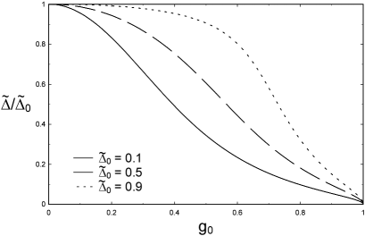
Figure 6: Numerical solution of Eq. (76) for $g_{c,0}=0$ as function of $g_{0}=g_{n,0}$ for different values of $\tilde{\Delta}_{0}=(k^{+}_{0}-k^{-}_{0})/\Lambda_{0}$.

The confinement transition for $g_{0}\rightarrow 1$ is clearly visible. In fact, the behavior of $\tilde{\Delta}$ for $g_{0}\rightarrow 1$ can be obtained analytically. In this case $\tilde{\Delta}\ll\sqrt{1-g_{0}^{2}}$, so that we may approximate

$$R(\tilde{\Delta}) \approx \frac{2}{\sqrt{1-g_{0}^{2}}}\ln\left[\frac{2\sqrt{1-g_{0}^{2}}}{\tilde{\Delta}}\right]\;.$$ (79)

The self-consistency condition (76) for $\tilde{\Delta}$ then reduces to

$$\tilde{\Delta}\approx\sqrt{1-g_{0}^{2}}\left[\frac{\tilde{\Delta}_{0}}{2\ln\left(\frac{2\sqrt{1-g_{0}^{2}}}{{\tilde{\Delta}}}\right)}\right]\;.$$ (80)

For $\tilde{\Delta}\ll\sqrt{1-g_{0}^{2}}$ the second factor in the square braces of Eq. (80) is small compared with unity, so that it is consistent to take the limit $g_{0}\rightarrow 1$ in this expression. If we identify $\Delta$ with the order parameter of the confinement transition transition (with $\Delta\neq 0$ corresponding to the deconfined phase), then Eq. (80) predicts mean-field behavior with logarithmic corrections.

Our simple one-loop approximation thus predicts that for $g_{0}\rightarrow 1$ there is a confinement transition where the true Fermi point distance $\Delta$ collapses, corresponding to vanishing effective interchain hoping $t_{\bot}^{\ast}=0$. In pseudo-spin language, the quantum critical point $g_{0}=1$ corresponds to a vanishing magnetization in $z$-direction, in spite of the fact that there is a uniform magnetic field. For $g_{0}>1$ our one-loop approximation suggests that there is long-range ferromagnetic order in $xy$-direction. However, in one dimension we do not expect true long-range order, so that fluctuations beyond the one-loop approximation should be important. It is therefore important to go beyond this approximation, which we shall do in the following subsection.

IV.3 Including the renormalization of the effective interaction

We now improve the above calculation by taking the flow of the effective interaction into account. For simplicity, we focus again on the special case without chiral interactions, so that we need to keep track only of the flowing non-chiral interaction $g_{n,l}=g_{l}$. Furthermore, in the absence of chiral couplings $r_{l}^{\sigma}=\sigma r_{l}$. The self-consistency equation (62) for the Fermi point distance then reduces to

$$\tilde{\Delta}=\tilde{\Delta}_{0}-\int_{0}^{\infty}dle^{-l}\frac{2\Theta(1-\tilde{\Delta}_{l})\tilde{\Delta}_{l}g_{l}^{2}}{\sqrt{1-g_{l}^{2}(1-\tilde{\Delta}_{l})^{2}}}\;,$$ (81)

where

$$\tilde{\Delta}_{l}=\tilde{\Delta}_{l}^{\ast}-2r_{l}=\tilde{\Delta}e^{l}-2r_{l}\;,$$ (82)

and the flow of $r_{l}$ and $g_{l}$ is determined by

$$\partial_{l}r_{l} = r_{l}+A(g_{l},\tilde{\Delta}_{l})\;,$$ (83)

$$\partial_{l}g_{l} = B(g_{l},\tilde{\Delta}_{l})\;,$$ (84)

with

$$A(g_{l},\tilde{\Delta}_{l})=\frac{\Theta(1-\tilde{\Delta}_{l})\tilde{\Delta}_{l}g_{l}^{2}}{\sqrt{1-g_{l}^{2}(1-\tilde{\Delta}_{l}^{2})}}\;,$$ (85)

and

$$B(g_{l},\tilde{\Delta}_{l}) = -2\eta_{l}g_{l}$$ (86)

$$=\frac{-2\Theta(1-\tilde{\Delta}_{l})g_{l}^{3}}{\sqrt{1-g_{l}^{2}(1-\tilde{\Delta}_{l}^{2})}\left[1+\sqrt{1-g_{l}^{2}(1-\tilde{\Delta}_{l}^{2})}\right]}\;.$$

The initial value $r_{0}$ has to be fine tuned such that $\lim_{l\rightarrow\infty}r_{l}$ remains finite. This leads to the self-consistency equation (81) for the true Fermi point distance. We emphasize again that our approximation scheme is not based on a weak coupling expansion, so that the $\beta$-function given in Eq. (86) is non-perturbative in the coupling $g_{l}$. Instead of Eq. (LABEL:eq:Rres1) we now obtain for the dimensionless renormalization factor $R(\tilde{\Delta})$ defined in Eq. (76),

$$R(\tilde{\Delta}) = \frac{2}{\tilde{\Delta}}\int_{0}^{\infty}dle^{-l}A(g_{l},\tilde{\Delta}_{l})$$ (87)

$$=2\int_{0}^{\infty}dl(1-2e^{-l}r_{l}/\tilde{\Delta})\frac{\Theta(1-\tilde{\Delta}_{l})g_{l}^{2}}{\sqrt{1-g_{l}^{2}(1-\tilde{\Delta}_{l}^{2})}}\;.$$

Note that formally the confinement transition manifests itself via a divergence of the function $R(\tilde{\Delta})$ for $\tilde{\Delta}\rightarrow 0$. However, as shown in Fig. 7, the renormalization factor remains now finite so that also the self-consistent $\tilde{\Delta}$ is finite for $g_{0}=1$, as shown in Fig. 8.

Figure 7: Numerical solution of the renormalization factor $R(\tilde{\Delta})$ defined in Eq. (87) as a function of the bare coupling $g_{0}$ for different values of $\tilde{\Delta}_{0}$.

Figure 8: Numerical solution of the true Fermi point distance $\tilde{\Delta}=(k^{+}-k^{-})/\Lambda_{0}$ as a function of the bare coupling $g_{0}$ for different values of the bare distance $\tilde{\Delta}_{0}=(k^{+}_{0}-k^{-}_{0})/\Lambda_{0}$.

We conclude that the confinement transition obtained in the previous subsection is an artefact of the approximations (72) and (73).

Let us take a closer look at the point $g_{0}=1$ where the one-loop approximation predicts a confinement transition. The RG flow of the couplings $g_{l}$ and $r_{l}$ as well as the flowing anomalous dimension $\eta_{l}$ for this case is shown in Fig. 9.

Figure 9: RG flow of the couplings $g_{l}$, $r_{l}$ and the anomalous dimension $\eta_{l}$ as a function of the logarithmic flow parameter $l$ for $\tilde{\Delta}_{0}=0.1$ and $g_{0}=1$.

One clearly sees that the initially large flowing anomalous dimension drives the running coupling $g_{l}$ towards smaller values; eventually $g_{l}$ approaches a finite limit for large $l$. Furthermore, the running coupling $r_{l}$ approaches its asymptotic value for large $l$ non-monotonously. The true Fermi point distance $\Delta$ as a function of the bare one for $g_{0}=1$ is shown in Fig. 10.

Figure 10: Numerical solution of the true Fermi point distance $\tilde{\Delta}$ for $g_{0}=1$ as a function of the bare distance $\tilde{\Delta}_{0}$.

We see that large interchain backscattering strongly reduces the Fermi point distance, although the Fermi surface never collapses, in agreement with scenario suggested by the weak coupling analysis Ledowski05 .

V Conclusions

In this work we have used a functional RG approach to calculate self-consistently the true distance $\Delta=k^{+}-k^{-}$ between the Fermi points of the bonding and the antibonding band in a system consisting of two chains of spinless fermions connected by weak interchain hopping $t_{\bot}$. Using the insight from our earlier weak coupling analysis Ledowski05 that the renormalization of the Fermi surface is essentially determined by interchain backscattering, we have treated this scattering process non-perturbatively by representing it in terms of a collective bosonic field $\chi$. In pseudospin language, where $t_{\bot}=h$ corresponds to a uniform magnetic field in $z$-direction and the interchain backscattering interaction corresponds to a ferromagnetic $xy$-interaction, the field $\chi$ can be viewed as a fluctuating transverse magnetic field, which competes with the uniform field $h$ in $z$-direction. A self-consistent one-loop approximation predicts that for sufficiently strong interchain backscattering there is indeed a quantum critical point were the renormalized Fermi point distance $\Delta\propto t_{\bot}^{\ast}$ vanishes. However, a more accurate calculation taking vertex corrections and wave-function renormalizations into account shows that the renormalized $\Delta\propto t_{\bot}^{\ast}$ remains finite. This is in agreement with the expectation that a ferromagnetic $xy$-interaction in a one-dimensional itinerant electron gas cannot give rise to long-range ferromagnetic order. Previous studies of the spinless two-chain problem Bourbonnais91 ; Caron02 came to the conclusion that the system exhibits a confinement transition if the anomalous dimension $\eta_{0}$ of the Luttinger liquid for $t_{\bot}=0$ is unity. The important difference between these earlier works and our calculations is that we have completely neglected pair tunneling. In a subsequent article Ledowski06 we shall show how the inclusion of this process stabilizes again the flow of the interchain backward scattering and enhances the tendency towards confinement. In the same article we shall also show that our approach can be generalized to study the more interesting and physically more relevant confinement problem in an infinite array of weakly coupled metallic chains. In this case the Fermi surface consists of two disconnected sheets, which self-consistently develop completely flat sectors at the confinement transition. We have preliminary evidence that in this case there exists a confined phase where the renormalized interchain hopping vanishes. The essential scattering process driving this transition is the non-chiral part of the density-density interaction which transfers momentum within a given sheet of the Fermi surface.

Finally we point out that this work describes also some technical progress: we have been able to find a sensible extrapolation of the weak coupling functional RG approach to the strong coupling regime. Our truncation strategy of the formally exact hierarchy of functional RG equations relies on the classification of the vertices according to their relevance. An obvious disadvantage of this approach is that we cannot give reliable error estimates, which is a common feature of most truncations of the coupled functional RG flow equations for the vertex functions. Note, however, that a similar truncation of the functional RG equations for the interacting Bose gas gave quite accurate results for the shift in the critical temperatureLedowski04 . In the present problem we know a priori from the weak coupling analysis that the physics is dominated by a single scattering channel, the inter-chain backscattering. However, an extension of our approach to problems where several scattering channels compete seems to be possible.

Appendix: Justification of the adiabatic approximation

We give here a justification for the adiabatic approximation for the rescaled spin-flip susceptibility given in Eq. (56). Let us therefore use a more general two-cutoff procedure where we impose a band-width cutoff $\Lambda^{F}_{\tau}=\Lambda_{0}^{F}e^{-\tau}$ on the fermionic propagator in addition to the bosonic momentum transfer cutoff $\Lambda_{l}=\Lambda_{0}e^{-l}$. All vertices and coupling constants then depend on both logarithmic flow parameters $l$ and $\tau$. Instead of Eq. (44) the rescaled fermionic propagator can then be approximated by

$$\tilde{G}_{l,\tau}^{\sigma}(q,i\epsilon,\alpha)\approx\frac{\Theta(1<|q|<e^{\tau})}{i\epsilon-\alpha\tilde{v}_{l,\tau}^{\sigma}q-r_{l,\tau}^{\sigma}}\;,$$ (A.88)

and the corresponding single-scale propagator is

$$\dot{\tilde{G}}_{l,\tau}^{\sigma}(q,i\epsilon,\alpha)\approx\frac{\delta(|q|-1)}{i\epsilon-\alpha\tilde{v}_{l,\tau}^{\sigma}q-r_{l,\tau}^{\sigma}}\;.$$ (A.89)

We recover the vertices of the momentum transfer cutoff scheme by taking first the limit $\tau\rightarrow\infty$. Of course, the result of the RG should be independent of how we reach a certain point in two-dimensional cutoff space spanned by $\Lambda_{l}$ and $\Lambda_{\tau}^{F}$. Suppose we first fix $\Lambda^{F}_{\tau}=\Lambda^{F}_{0}$ and perform the reduction of the momentum transfer cutoff $\Lambda_{0}\rightarrow\Lambda_{l}$. As a second step we reduce the fermionic cutoff $\Lambda^{F}\rightarrow 0$. On the right-hand side of the flow equation for the spin-flip susceptibility there are then two additional diagrams Schuetz05 involving the fermionic single-scale propagator, which are shown in Fig. 11.

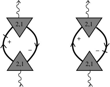
Figure 11: Additional diagrams contributing to the flow of the spin-flip susceptibility in a cutoff scheme with a fermionic band-width cutoff. The solid arrow with slash is the fermionic single-scale propagator.

For a fixed scale $l$ the corresponding flow equation is (for simplicity we set $\alpha=1$ and omit the chirality label)

$$\partial_{\tau}\tilde{\Pi}^{\sigma\bar{\sigma}}_{l,\tau}(\bar{Q}) = -[\bar{q}\partial_{\bar{q}}+\bar{\epsilon}\partial_{\bar{\epsilon}}]\tilde{\Pi}^{\sigma\bar{\sigma}}_{l,\tau}(\bar{Q})+\dot{{\Pi}}^{\sigma\bar{\sigma}}_{l,\tau}(\bar{Q}),$$ (A.90)

with

$$\dot{\Pi}^{\sigma\bar{\sigma}}_{l,\tau}(\bar{Q}) = -{\gamma}_{l,\tau}^{2}\int_{Q}\Bigl{[}\dot{\tilde{G}}_{l,\tau}^{\sigma}({Q}){\tilde{G}}^{\bar{\sigma}}_{l,\tau}(Q+\bar{Q}+\sigma\tilde{\Delta}^{\ast}_{\tau})$$ (A.91)

$$+{\tilde{G}}_{l,\tau}^{\sigma}({Q})\dot{\tilde{G}}^{\bar{\sigma}}_{l,\tau}(Q+\bar{Q}+\sigma\tilde{\Delta}_{\tau}^{\ast})\Bigr{]}\;,$$

where $\tilde{\Delta}_{\tau}^{\ast}=\Delta/\Lambda_{\tau}^{F}$. The flow equation for the spin-flip vertex is now of the form

$$\partial_{\tau}{\gamma}_{l,\tau}=\Theta(\lambda+l-\tau)C(l,\tau)\;,$$ (A.92)

where $C(l,\tau)$ is some function of the flow parameters and of the running coupling constants, and $\lambda=\ln(\Lambda_{0}^{F}/\Lambda_{0})$. For simplicity we choose $\Lambda_{0}=\Lambda_{0}^{F}$, so that $\lambda=0$. The $\Theta$-function is due to the fact that the internal loop momenta are restricted by the momentum transfer cutoff $\Lambda_{0}$. Obviously, $\partial_{\tau}{\gamma}_{l,\tau}=0$ for $\tau>l$, so that $\gamma_{l}\equiv\gamma_{l,\tau>l}$ is independent of $\tau$. Similarly, the flow equation for $r_{l,\tau}^{\sigma}$ is of the form

$$\partial_{\tau}{r}^{\sigma}_{l,\tau}={r}^{\sigma}_{l,\tau}+\Theta(l-\tau)A(l,\tau)\;,$$ (A.93)

with some other function $A(l,\tau)$. This implies $r_{l,\tau}^{\sigma}=e^{\tau-l}r^{\sigma}_{l,\tau=l}$ for $\tau>l$, so that the flowing Fermi point distance $\tilde{\Delta}_{l,\tau}$, defined analogous to Eq. (57) via

$$\tilde{\Delta}_{l,\tau}=\frac{\Delta}{\Lambda_{\tau}^{F}}-(r^{+}_{l,\tau}-r^{-}_{l,\tau})\;,$$ (A.94)

is for $\tau>l$ of the form

$$\tilde{\Delta}_{l,\tau>l} = \frac{\Delta}{\Lambda_{\tau}^{F}}-e^{(\tau-l)}(r^{+}_{l,l}-r^{-}_{l,l})$$ (A.95)

$$= e^{\tau-l}\left[\frac{\Delta}{\Lambda_{l}}-(r^{+}_{l}-r^{-}_{l})\right]$$

$$= e^{\tau-l}\tilde{\Delta}_{l}\;,$$

where we have defined $r_{l}^{\sigma}=r_{l,\tau=l}^{\sigma}$ and $\tilde{\Delta}_{l}=\Delta/\Lambda_{l}-(r_{l}^{+}-r_{l}^{-})$, see Eq. (57). For $\tau\rightarrow\infty$ the solution of Eq. (A.90) can therefore be written as

$$\tilde{\Pi}^{\sigma\bar{\sigma}}_{l}(\bar{Q}) = \int_{0}^{\infty}\!\!\!d\tau\>\dot{\Pi}^{\sigma\bar{\sigma}}_{l,\tau}(\bar{Q}e^{\tau-l};\tilde{\Delta}_{l,\tau})$$ (A.96)

$$= \int_{0}^{{l}}\!\!\!d\tau\>\dot{\Pi}^{\sigma\bar{\sigma}}_{l,\tau}(\bar{Q}e^{\tau-l};\tilde{\Delta}_{l,\tau})$$

$$+ \int_{{l}}^{\infty}\!\!\!d\tau\;\dot{\Pi}^{\sigma\bar{\sigma}}_{l,\tau}(\bar{Q}e^{\tau-l};\tilde{\Delta}_{l}e^{\tau-l})\;.$$

Using the fact that in the integral of the last term we may pull out a factor of $\gamma_{l}^{2}$ and approximating the fermionic Green functions by Eqs. (A.88) and (A.89) with $\tilde{v}^{\sigma}_{l,\tau}$ and $r_{l,\tau}$ set equal to zero, we recover from the last term the adiabatic approximation (56). Actually, to calculate the flow of the fermionic self energy, we only need the bosonic Green function at $q=\pm 1$. For $\tilde{\Delta}_{l}<1$ the non-adiabatic contribution to the polarization then vanishes, leaving us just with the adiabatic part. For larger $\tilde{\Delta}_{l}$ there is a crossover to the more general expression. However, the leading contribution to the flow of $\tilde{\Delta}_{l}$ itself stems from the region where the adiabatic approximation is valid.

Finally we note that the adiabatic approximation (56) is also consistent with the flow equation for the spin-flip susceptibility in the momentum transfer cutoff scheme shown in Fig. 4: taking the derivative of the right-hand side of Eq. (56) with respect to the flow parameter and inserting for the derivative of the fermionic self-energy its flow equation (14), we find that the right-hand side can be written in terms of a symmetrized closed fermion loop with four bosonic legs and renormalized propagators. This corresponds to the adiabatic approximation for the vertex $\Gamma^{(0,4)}_{\Lambda}$ which according to Fig. 4 drives the flow of the spin-flip susceptibility.

References

- (1) I. J. Pomeranchuk, Zh. Eksp. Teor. Fiz. 35, 524 (1958) [Sov. Phys. JETP 8, 361 (1958)].
- (2) I. M. Lifshitz, Zh. Eksp. Teor. Fiz. 38, 1569 (1960) [Sov. Phys. JETP 11, 1130 (1960)].
- (3) J. Quintanilla and A. J. Schofield, Phys. Rev. B 74, 115126 (2006).
- (4) A. Luther, Phys. Rev. B 50, 11446 (1994).
- (5) A. T. Zheleznyak, V. M. Yakovenko, and I. E. Dzyaloshinskii, Phys. Rev. B 55, 3200 (1997).
- (6) A. Ferraz, Phys. Rev. B 68, 075115 (2003); H. Freire, E. Correa, and A. Ferraz, Phys. Rev. B 71, 165113 (2005).
- (7) C. Honerkamp, M. Salmhofer, N. Furukawa, and T. M. Rice, Phys. Rev. B 63, 035109 (2001).
- (8) S. Ledowski and P. Kopietz, unpublished.
- (9) A. Neumayr and W. Metzner, Phys. Rev. B 67, 035112 (2003).
- (10) S. Dusuel and B. Douçot, Phys. Rev. B 67, 205111 (2003).
- (11) J. Feldman, M. Salmhofer, and E. Trubowitz, J. Stat. Phys. 84, 1209 (1996); Commun. Pure Appl. Math. 51, 1133 (1998); ibid. 52, 273 (1999).
- (12) P. Kopietz and T. Busche, Phys. Rev. B 64, 155101 (2001).
- (13) S. Ledowski and P. Kopietz, J. Phys.: Condens. Matter 15, 4779 (2003).
- (14) S. Ledowski, P. Kopietz, and A. Ferraz, Phys. Rev. B 71, 235106 (2005).
- (15) F. Schütz, L. Bartosch, and P. Kopietz, Phys. Rev. B 72, 035107 (2005); F. Schütz and P. Kopietz, J. Phys. A: Math. Gen. 39, 8205 (2006).
- (16) M. Fabrizio, Phys. Rev. B 48, 15838 (1993).
- (17) S. A. Brazovskii and V. M. Yakovenko, Zh. Eksp. Teor. Fiz. 89, 2318 (1985) [Sov. Phys. JETP 62, 1340 (1985)].
- (18) C. Bourbonnais and L. G. Caron, Int. J. Mod. Phys. B 5, 1033 (1991).
- (19) F. Kusmartsev, A. Luther, and A. A. Nersesyan, Pis’ma Zh. Eksp. Teor. Fiz. 55, 692 (1992) [JETP Lett. 55, 724 (1992)]; V. M. Yakovenko, ibid. 56, 523 (1992) [56, 510 (1992)].
- (20) A. M. Finkelstein and A. I. Larkin, Phys. Rev. B 47, 10461 (1993).
- (21) D. Boies, C. Bourbonnais and A.-M. S. Tremblay, Phys. Rev. Lett. 74, 968 (1995).
- (22) L. Balents and M. P. A. Fisher, Phys. Rev. B 53, 12133 (1996); H.-H. Lin, L. Balents, and M. P. A. Fisher, Phys. Rev. B 56, 6569 (1997).
- (23) E. Arrigoni, Phys. Rev. Lett. 80, 790 (1998); Phys. Rev. B 61, 7909 (2000).
- (24) U. Ledermann and K. Le Hur, Phys. Rev. B 61, 2497 (2000).
- (25) K. Louis, J. V. Alvarez, and C. Gros, Phys. Rev. B 64, 113106 (2001); K. Hamacher, C. Gros, and W. Wenzel, Phys. Rev. Lett. 88, 217203 (2002).
- (26) L. G. Caron and C. Bourbonnais, Phys. Rev. B 66, 045101 (2002).
- (27) C. Bourbonnais, B. Guay, and R. Wortis, in Theoretical Methods for Strongly Correlated Electrons, ed. D. Sénéchal, A. M. Tremblay and C. Bourbonnais (Springer-Verlag, New York, 2004).
- (28) J. C. Nickel, R. Duprat, C. Bourbonnais, and N. Dupuis, Phys. Rev. B 73, 165126 (2006).
- (29) M. Tsuchiizu, Phys. Rev. B 74, 155109 (2006).
- (30) There are several possibilities to write the Hubbard interaction in the form (LABEL:eq:action1). One possibility is to set and , where is the lattice spacing. An alternative is and . This freedom translates into similar ambiguities in the choice of decoupling of the Hubbard interaction in terms of bosonic collective fields. For a discussion of this point see C. A. Macêdo and M. D. Coutinho-Filho, Phys. B 43, 13515 (1991), and S. De Palo, C. Castellani, C. Di Castro, and B. K. Chakraverty, Phys. Rev. B 60, 564 (1999).
- (31) J. Solyom, Adv. Phys. 28, 201 (1979).
- (32) C. Wetterich, Phys. Lett. B 301, 90 (1993).
- (33) T. R. Morris, Int. J. Mod. Phys. A 9, 2411 (1994).
- (34) C. Wetterich, cond-mat/0208361v3.
- (35) T. Baier, E. Bick, and C. Wetterich, Phys. Rev. B 70, 125111 (2004).
- (36) M. Salmhofer and C. Honerkamp, Prog. Theor. Physics 105, 1 (2001).
- (37) J. Polchinski, Nucl. Phys. B 231, 269 (1984).
- (38) S. Ledowski, N. Hasselmann, and P. Kopietz, Phys. Rev. A 69, 061601(R) (2004); N. Hasselmann, S. Ledowski, and P. Kopietz, ibid. 70, 063621 (2004).