Optical Sum Rule in Finite Bands

Abstract

In a single finite electronic band the total optical spectral weight or optical sum carries information on the interactions involved between the charge carriers as well as on their band structure. It varies with temperature as well as with impurity scattering. The single band optical sum also bears some relationship to the charge carrier kinetic energy and, thus, can potentially provide useful information, particularly on its change as the charge carriers go from normal to superconducting state. Here we review the considerable advances that have recently been made in the context of high $T_{c}$ oxides, both theoretical and experimental.

I Introduction

Much is known about the properties of the superconducting state in the cuprates, yet after 20 years of intense research there is, as yet, no consensus as to the driving interactions responsible for the pairing (mechanism). It is well established that the superconducting order parameter has $d$-wave rather than conventional $s$-wave symmetry. Angular resolved photoemission spectroscopyref1 ; ref2 (ARPES) finds that the leading edge of the electron spectral density at the Fermi energy shifts below the chemical potential as a result of the onset of superconductivity. The observed shift is zero in the nodal direction $(\pi,\pi)$ and maximum in the antinodal direction $(0,\pi)$. More recently a non monotonic increase of the gap amplitude as a function of direction has been observed in an electron doped cuprate but the symmetry is again $d$-wave.ref3

Many other independent experimental techniques have provided additional compelling evidence for $d$-wave symmetry. One such technique is microwave spectroscopy which gives a linear in temperature $(T)$ dependence of the superfluid density at low $T$ [ref4, ]. Complimentary to the above techniques are phase sensitive experimentsref5 based on Josephson tunneling and flux quantization which provide direct evidence for a change in sign of the order parameter not just that it has a zero.

Another important observation which points directly to a non conventional mechanism is the so called collapse of the inelastic scattering rateref6 ; ref7 ; ref8 ; ref9 in the superconducting state which results in a large peak at intermediate $T$ below the critical temperature $(T_{c})$ in the real part of the microwave conductivity.ref6 ; ref7 ; ref10 ; ref11 The origin of this peak is understood in terms of a readjustment in the excitation spectrum involved in the interaction as superconductivity develops. This is expected in electronic mechanismsref6 ; ref9 involving the spin or charge susceptibility which looses weight at small energies corresponding to a hardening of the spectrum and little inelastic scattering remains at low $T$.

All the evidence reviewed above points to deviations from a simple BCS $s$-wave phonon driven superconductivity, but, nevertheless, the search goes on for other essential differences which could help identify the underlying mechanism. An avenue to explore is the idea of kinetic as opposed to potential energy driven superconductivity. The idea is that it is a reduction in kinetic energy (KE) that drives the condensation into the superconducting state in contrast to BCS theory where the potential is decreased sufficiently to overcome a KE increase and provides as well a reduction in total energy. The possibility of KE driven superconductivity was considered by Hirschref12 and explicitely demonstrated for the hole mechanism of superconductivityref13 ; ref14 ; ref15 for which the effective mass of the holes decreases in the superconducting state by pairing. It is also expected in other theoretical frameworks for highly correlated systems.ref16 ; ref17

In a single finite tight binding band with nearest neighbors hopping only, the KE is related to the optical sum defined as the total optical spectral weight under the real part of the optical conductivity $\sigma_{1}(T,\omega)$ integrated over energy $\omega$.ref19 This fact applies whatever the interactions involved, the temperature, and also when impurities are present. Of course, for this to hold the conductivity needs to be computed exactly including vertex corrections. At first sight the restriction to a tight binding band with nearest neighbors only appears restrictive but in reality it has been found that KE and optical sum (OS) track each other reasonably well even when higher neighbors are considered (second, third, etc.). In view of this fact several recent experimental and theoretical papers have appeared concerning the temperature dependence of the OS in the normal state and its change in the superconducting state. Here, we review this body of work with the aim of understanding what it tells us about the underlying interactions involved. We will restrict our discussion to the cuprates and to their in-plane response. For the $c$-axis motion a sum rule violation was noticed by Basov et al.ref18 but the KE involved in the $c$-axis motion is small.ref20 ; ref21 To investigate its relation to the total condensation energy of the transition to the superconducting state, it is necessary to consider the $ab$-plane of the cuprates. Exactly how to treat the $c$-axis transport also complicates the interpretation. Some possible mechanisms include strong intra layer scattering,ref22 non Fermi liquid ground states,ref23 confinement,ref16 inter-plane and in-plane charge fluctuations,ref24 indirect $c$-axis coupling through the particle-particle channel,ref25 resonant tunneling on localized states in the blocking layer,ref26 two band models,ref27 ; ref28 and coherent and incoherent tunneling.ref29 ; ref30 ; ref31 ; ref32 ; ref33 Clearly this problem is worth further study but is not part of this review which will deal only with the cuprates and their $ab$-plane response.

The in-plane optical sum (OS) in the cuprates is observed to increase as the temperature is decreased below room temperature. In the normal phase it is often, but not always, found to follow a $T^{2}$ law. The changes are small but larger than is expected on a rigid band model neglecting interactions. In the superconducting phase, on the other hand, a change in slope of this $T^{2}$ behavior is seen. While there remain some differences in details between the various experimental groups, for underdoped samples it is agreed that the OS falls above the extrapolated normal state value. This is clearly seen in Fig. 14 which was reproduced from van der Marel et al.ref34 and deals with Bi₂Sr₂CaCu₂O_8+x (BSCCO, Bi2212). This behavior is opposite to that expected on the basis of BCS theory for which the OS is predicted to decrease. This fact can be traced to an increase in KE due to the formation of Cooper pairs. On the other hand, such a conventional behavior of the OS or change in KE on entering the superconducting state was observed in overdoped samples of BSCCO by Deutscher et al.ref87a Their data is reproduced in our Fig. 20. These authors also find that the crossover from negative to positive KE change occurs around, but slightly above optimum doping (see Fig. 21). These findings have been largely confirmed by Carbone et al.ref33a It is these facts that this review is directly concerned with and seeks to understand. Theoretically we will find that the temperature dependence of the OS can in some cases be dominated by a term which is proportional to a specific average over energy of the quasiparticle inelastic scattering rates and this need not give a $T^{2}$ law. This term is missing in all theories that do not explicitly treat damping effects. Further, this non $T^{2}$ dependence has implications for the accuracy of experimental results on the OS difference between superconducting and normal state which require an extrapolation to low temperatures of normal state data known only above $T_{c}$.

The paper is structured as follows. We begin with theoretical considerations and then review experimental information as it relates to the calculations. Section II.1 introduces the optical sum and its relation to the kinetic energy. In Sec. II.2 we provide simple analytic formulas for the KE and OS in a free electron model which allows one to understand some qualitative aspects of this relationship. It also contains a general formulation of the OS for a simplified tight binding model which averages over anisotropies and greatly simplifies the mathematics. We argue that the temperature dependence of the OS is governed mainly by the inelastic scattering. Both, real and imaginary part of the charge carrier self energy are important. In Sec. II.3 we describe the Nearly Antiferromagnetic Fermi Liquid model (NAFFL), give the set of generalized Eliashberg equations needed for numerical work, and also specify the electron-spin fluctuations interaction (MMP model). We give results for the temperature dependence of the OS and of the KE in the normal and superconducting state. In Sec. II.4 we introduce the Hubbard model and Dynamical Mean Field Theory (DMFT) and give results.

In Sec. III.1 we summarize some of the important effects a finite band cutoff has on the self energy. Section III.2 is devoted to results for the OS when a delta function, and Sec. III.3 when an MMP form (spin fluctuations) is used for the electron-boson interaction. Section III.4 provides an analysis of the temperature dependence of the OS for coupling to a low energy boson which results in a linear rather than quadratic in $T$ law. It is argued that other temperature dependences could arise when different model interactions are used.

In Sec. IV.1 we investigate within the NAFFL model the effect on the OS of the collapse of the inelastic scattering on entering the superconducting state which can lead to an increase in the OS rather than the usual BCS behavior. We also present experimental results in the BSCCO cuprates. Section IV.2 deals with a simplified qualitative model based on a temperature dependent scattering rate which decreases with $T$ as $T^{4}$. While this model is not accurate, it shows clearly how the KE in the superconducting state can decrease below its normal state value due to the collapse of the inelastic scattering. In Sec. IV.3 we describe a related, more phenomenological model due to Norman and Pépin which has several common elements with the model discussed in Sec. IV.1. We also provide comparison with experiment and additional theoretical results for the KE change on condensation into the superconducting state in Sec. IV.4. Section IV.5 gives DMFT results for the normal as well as superconducting state in the $t$-$J$ model. KE and potential energy are discussed and compared with experiment. Further results based on the Hubbard model are commented on as are those based on the negative $U$ Hubbard model used to describe the BCS - BE (Bose - Einstein) crossover.

Section V deals with models of the pseudogap state above $T_{c}$ (the superconducting critical temperature) that exists up to a temperature $T^{\ast}>T_{c}$, with $T^{\ast}$ the pseudogap temperature. In Sec. V.1 we discuss KE changes in the preformed pair model in which pairs form at the pseudogap temperature $T^{\ast}$ and superconductivity sets in only at a lower temperature when phase coherence is established. In Sec. V.2 we consider an alternative model to phase fluctuations of the pseudogap state, namely the $D$-density wave model, a competing ordered state with bond currents and associated magnetic moments. In Sec. VI we deal briefly with the problem of spectral weight distribution as a function of energy. A short summary is provided in Sec. VII.

II THEORY

II.1 General considerations

The single band OS is defined asref34

$$\int\limits_{-\Omega}^{\Omega}\!d\omega\,\Re{\rm e}[\sigma_{1xx}(\omega)]=\frac{\pi e^{2}}{\hbar^{2}V}\sum\limits_{{\bf k},\sigma}n_{{\bf k},\sigma}\frac{\partial^{2}\varepsilon_{\bf k}}{\partial k_{x}^{2}}=\frac{\pi e^{2}}{\hbar^{2}}W.$$ (1)

Here $\sigma_{1xx}(\omega)$ is the real part of the $(x,x)$-component of the optical conductivity, $e$ is the electron charge, $\hbar$ Planck’s constant, k momentum, $\sigma$ spin, and $V$ the crystal volume. The limits $-\Omega$ to $\Omega$ on the conductivity integral are to be taken to include all the contributions to $\sigma_{1xx}(\omega)$ from the band of interest and from no other. The integration from $-\Omega$ to $\Omega$ can be restricted to $(0,\Omega)$ by making use of the fact that the real part of the conductivity is an even function of $\omega$. Often the integration on $\Omega$ is also extended to infinity under the condition that only transitions from the one band of interest are included. The sum over k extends over the entire first Brillouin zone, $n_{{\bf k},\sigma}$ is the probability of occupation of a state $|{\bf k},\sigma\rangle$, and $\varepsilon_{\bf k}$ is the electron dispersion relation. $W$ is the OS divided by $\pi e^{2}/\hbar^{2}$ and will be quoted in meV. In deriving this OS rule the one body part of the Hamiltonian gives the single particle orbitals of energy $\varepsilon_{\bf k}$ and the two body piece provides correlation effects beyond those included in

Table 1: The two tight binding models used within this paper. Model A corresponds to the tight binding model discussed by van der Marel et al.ref34 $t$ and $t^{\prime}$ are given in meV, the critical temperature $T_{c}$ in K, and the filling $\langle n\rangle$ is defined in Eq. (22).

Model	$t$	$t^{\prime}$	$\langle n\rangle$	$T_{c}$
A	$148.8$	$40.9$	$0.425$	$90$
B	$100.0$	$16.0$	$0.4$	$100$

$\varepsilon_{\bf k}$ (referred to as kinetic energy even though it can contain effects of interactions). If all bands are included rather than just the one in Eq. (1) one would obtain the exact sum rule proportional to $n/m$ with $m$ the bare electron mass and $n$ the total electron density. This is a constant independent of temperature. It does not change when the system undergoes a phase transition to the superconducting state by charge conservation. This also applies to the free electron infinite band and is the basis for the Ferrell-Glover-Tinkham sum ruleref123 ; ref124 which will be elaborated upon in Sec. VI.

Figure 1: Optical sum $W$ and kinetic energy, $-W_{\rm KE}/2$, as a function of $T^{2}$. Solid circles and squares are for the non interacting case while solid up-triangles and solid down-triangles include interactions. The left hand frame applies to Model A of Table 1 and an MMP model parameter $\omega_{SF}=82\,$meV [see Eq. (19)] was used. Here, the interacting and non interacting cases show similar temperature dependencies. The right hand frame is for Model B of Table 1 with an MMP model parameter $\omega_{SF}=10\,$meV. Note the difference in temperature dependence between interacting and non interacting case.

The important observation for this review is that for tight binding bands with nearest neighbors hopping, $t$, only, i.e.:

$$\varepsilon_{\bf k}=-2t\left[\cos(ak_{x})+\cos(ak_{y})\right],$$ (2)

where $a$ is the CuO₂ plane lattice parameter,

$$W\equiv-\frac{1}{2}W_{KE}\equiv-\frac{1}{2}\frac{a^{2}}{V}\sum\limits_{{\bf k},\sigma}n_{{\bf k},\sigma}\varepsilon_{\bf k}.$$ (3)

$W_{KE}$ is the kinetic energy per copper atom. Thus, for this simple case an experimental measurement of $W$ gives a measure of the KE. The band structure in the oxides is not, in general, limited to first neighbor hopping and one may well wonder if the above observation is of any practical use.

For second neighbor hopping ($t,\,t^{\prime}$ model)

$$\varepsilon_{\bf k} = -2\left\{t\left[\cos(ak_{x})+\cos(ak_{y})\right]\right.$$ (4)

$$\left.-2t^{\prime}\cos(ak_{x})\cos(ak_{y})\right\}-\mu,$$

with $\mu$ the chemical potential. In Fig. 1 we compare results for $W$ (solid circles) with results for $-W_{KE}/2$ (solid squares) for two models, A and B, left and right hand frame, respectively. Parameters of the models are defined in Table 1 where $\langle n\rangle$ is the filling factor which determines the chemical potential; with $\langle n\rangle=0.5$, half filling, $\mu=0$ and $t^{\prime}=0$ in Eq. (4). No interactions are included beyond those giving rise to the tight binding band structure. It is clear that while $W$ in both cases is a few percent smaller than $-W_{KE}/2$ their dependence on temperature track each other fairly well. Thus, it makes sense to pursue this avenue as a means to get information on the KE and its variation with temperature and also when it undergoes a phase transition to the superconducting state. One should be aware, however, that for some sets of tight binding parameters the difference between OS and KE can be much larger and they may no longer track each other (see the very recent paper by Marsiglio et al.ref124a for more discussion). A final point should be stressed. To compute the OS in Eq. (1) it is not necessary, although one can if one wishes, to calculate the conductivity which depends on a two-particle Green’s function and is to be calculated with vertex corrections. The right hand side of Eq. (1), instead, depends only on the one particle spectral density $n_{{\bf k},\sigma}$ which determines the probability of occupation of the state $|\textbf{k},\sigma\rangle$. On the other hand, if one is interested in the optical spectral weight integrated only to $\omega_{M}$ with $\omega_{M}<\Omega$ one can no longer avoid calculating the conductivity. For this reason the problem of optical weight distribution is left to a last section VI.

II.2 The Continuum Limit and Quadratic Dispersion; Simple Results

To get some insight into the significance of the OS, we consider next several simplifications. The probability of occupation of the state $|{\bf k}\rangle$ (both spins) is related to the charge carrier spectral density $A({\bf k},\omega)$ by

$$n_{\bf k}(T)=\int\limits_{-\infty}^{\infty}\!d\omega\,f(T,\omega)A({\bf k},\omega),$$ (5)

where $f(T,\omega)$ is the Fermi-Dirac distribution function at temperature $T$. For tight binding electrons with no correlation effects the spectral function $A({\bf k},\omega)=\delta(\varepsilon_{\bf k}-\omega)$ and $n_{\bf k}(T)=f(\varepsilon_{\bf k},T)$. Before proceeding to include interactions it is convenient in what follows to rewrite Eq. (1) in an equivalent form through integration by parts with the surface integral equal to zero by symmetry in a periodic band:

$$\bar{W}=-\frac{2}{V}\sum\limits_{\bf k}\left(\frac{\partial\varepsilon_{\bf k}}{\partial{\bf k}}\right)^{2}\frac{dn_{\bf k}}{d\varepsilon_{\bf k}}.$$ (6)

Knigavko et al.ref49 have found this second form to be very useful when making approximations. In the Kubo formula which defines the conductivity $\sigma_{1xx}(\omega)$ which appears on the left hand side of Eq. (1) it is the velocity squared, $(\partial\varepsilon_{\bf k}/\partial k_{x})^{2}$ that enters naturally. In making approximations to the band structure in order to get simplified expressions it is important to have the same quantity $(\partial\varepsilon_{\bf k}/\partial k_{x})^{2}$ on both sides of Eq. (1) and, indeed, in Ref. ref49, it is verified that the right hand side (RHS) of Eq. (1) and $\bar{W}$ of Eq. (6) agree to high accuracy for the two simplified band structure models they considered, namely free electron bands cut off to $-D/2$ and $D/2$ at half filling and another model designed to treat the tight binding case which we will define later. In both cases the density of states was approximated by a constant. Such an approximation, however, is not completely compatible with the assumed Fermi velocity model and this explains why we use $\bar{W}$ rather than $W$. In the continuum limit of Eq. (4) with $t^{\prime}=\mu=0$ as the lattice parameter $a\to 0$ one gets

$$\varepsilon_{\bf k}=-4t+\frac{\hbar^{2}}{2m}\left(k_{x}^{2}+k_{y}^{2}\right),$$

with $\hbar^{2}/2m=ta^{2}$ (where this product is assumed to be finite as $a\to 0$) or $a^{2}=\frac{\hbar^{2}}{m}\frac{4}{D}$ and $D/2=4t$. For these approximations

$$W=\bar{W}=\frac{(\hbar\Omega_{p})^{2}}{4\pi e^{2}},$$

the well known result for free electron bands, with $\Omega^{2}_{p}=4\pi ne^{2}/m$ the plasma frequency squared and $n$ the electron density. We can also show that

$$W_{KE}=-W,$$

so that the relationship between KE and OS found for tight binding bands with first neighbors is profoundly changed when these are approximated by their continuum limit (free electron case). This is, in a sense, the extreme opposite case to the nearest neighbor only tight binding model. These results were obtained at zero temperature. At finite $T$ things are not quite as simple. $W$ and $\bar{W}$ undergo no change with temperature but $W_{KE}$ does and is

$$W_{KE}=\frac{N(0)D\hbar^{2}}{m}\left[\frac{\pi^{2}}{3}\left(\frac{k_{B}T}{D/2}\right)^{2}-1\right],$$

which is the well known result that the KE increases as the square of the temperature normalized to the half band width $D/2$. These results show that the correspondence between $W$ and $W_{KE}$ can be rather subtle and it can be lost when approximations to the tight binding band are made. Here $N(0)$ is the charge carrier density of states at the Fermi energy.

Knigavko et al.ref49 used a somewhat more sophisticated model to approximate a tight binding band. This model was used previously by Marsiglio and Hirsch.ref50 In this approach the square of the electron velocity is replaced by

$$\left(\frac{1}{\hbar}\frac{\partial\varepsilon_{\bf k}}{\partial k_{x}}\right)^{2}=\frac{D}{4m_{b}}\left[1-\left(\frac{\varepsilon_{\bf k}}{D/2}\right)^{2}\right]$$

and

$$\bar{W}(T)=\frac{\hbar^{2}}{m_{b}}\left(-\int\limits_{-\infty}^{\infty}\frac{d\omega}{D/2}\,f(T,\omega)\int\limits_{-D/2}^{D/2}\frac{d\epsilon}{D/2}\,\epsilon A(\epsilon,\omega)\right).$$ (7)

Here, $m_{b}$ is a band electronic mass. In this model the rule that $\bar{W}=-W_{KE}/2$ still holds. For $A(\epsilon,\omega)=\delta(\epsilon-\omega)$ (no correlations) we recover

$$\bar{W}(T)=\frac{\hbar^{2}}{m_{b}}\left[1-\frac{1}{3}\left(\frac{k_{B}T}{D/2}\right)^{2}\right],$$ (8)

which is a result obtained by van der Marel et al.ref34 and often used to interpret experiments. It is important to contrast this result with the free electron case for which

$$\left(\frac{1}{\hbar}\frac{\partial\varepsilon_{\bf k}}{\partial k_{x}}\right)^{2}=\frac{D/2+\varepsilon_{\bf k}}{m}$$

and

$$\bar{W}(T)=\frac{\hbar^{2}n}{m}\left[1-\frac{2}{n}\int\limits_{-\infty}^{\infty}\!d\omega\,f(T,\omega)A(D/2,\omega)\right],$$ (9)

where $n$ is the charge carrier density.

To treat interactions it is convenient to rewrite Eq. (7) in the form

$$\bar{W}(T)=\frac{\hbar^{2}}{2m_{b}}\left[1-\int\limits_{-\infty}^{\infty}\!d\omega\,f(T,\omega)h(T,\omega)\right],$$ (10)

where

$$h(T,\omega)=\frac{4}{(D/2)^{2}}\int\limits_{0}^{D/2}\!d\epsilon\,\epsilon A(\epsilon,\omega).$$ (11)

Note also that the probability of occupation of the state $\epsilon$ given in Eq. (5) is closely related to Eqs. (10) and (11). We can apply the Sommerfeld expansion to Eq. (11) to get

$$\bar{W}(T) = \frac{\hbar^{2}}{2m_{b}}\left[1-\int\limits_{-\infty}^{0}\!d\omega\,h(T,\omega)-\frac{\pi^{2}}{6}\left(k_{B}T\right)^{2}\right.$$ (12)

$$\times\left.\left.\frac{d\,h(T,\omega)}{d\,\omega}\right|_{\omega=0}\right].$$

For no interactions $h(T,\omega)=4\omega/(D/2)^{2}$ for $\omega\geq 0$ and zero for $\omega<0$ [note that the derivative in Eq. (12) (non interacting case) is to be weighted by $1/2$ at $\omega=0$] so that the second term in Eq. (12) vanishes and the third term gives the first correction in (8). In terms of the real and imaginary part of the self energy we can work out $h(T,\omega)$ to get

$$h(T,\omega) = \frac{4}{\left(\frac{D}{2}\right)^{2}}\left\{\frac{\chi}{\pi}\left[\tan^{-1}\left(\frac{\frac{D}{2}-\chi}{y}\right)+\tan^{-1}\left(\frac{\chi}{y}\right)\right]\right.$$ (13)

$$\left.+\frac{y}{2\pi}\ln\left|\frac{y^{2}+\left(\frac{D}{2}-\chi\right)^{2}}{y^{2}+\chi^{2}}\right|\right\},$$

where $\chi=\omega-\Sigma_{1}(\omega)$ and $y=-\Sigma_{2}(\omega)$ with $\Sigma_{1}(\omega)$ [$\Sigma_{2}(\omega)$] the real [imaginary] part of the self energy $\Sigma(\omega)$. If the real part of $\Sigma$ is neglected and its imaginary part is assumed to be a constant $\Gamma$ as it would be for impurities in an infinite band we can work out the integral in Eq. (12) and get:

$$\bar{W}(T)=\frac{\hbar^{2}}{2m_{b}}\left[1-\frac{8\Gamma}{D\pi}-\frac{\pi^{2}}{3}\left(\frac{k_{B}T}{D/2}\right)^{2}\right].$$ (14)

Note that the second term which deals directly with interactions between the electrons is of order some scattering rate over $D/2$ while the third which has often been emphasized in literature, is of order $[k_{B}T/(D/2)]^{2}$ and, therefore, can be expected to be much smaller than the first. In the oxides, as an example, $\Gamma$ is known to be of order $T$.ref126 Eq. (14) was arrived at independently by Benfatto et al.ref52 and by Karakozov and Maksimov.ref53 It is central to any discussion of single band sum rule. While the approach taken in Refs. ref52, and ref53, are somewhat different much of the basic content is similar.

Finally, we consider the superconducting state at $T=0$ for which in BCS theory

$$n_{\bf k}=\frac{1}{2}\left(1-\frac{\varepsilon_{\bf k}}{\sqrt{\varepsilon_{\bf k}^{2}+\Delta_{\bf k}^{2}}}\right),$$ (15)

where the gap $\Delta_{\bf k}$ can have $d$-wave symmetry of the form $\Delta_{\bf k}=\Delta\cos(2\phi)$. Here $\Delta$ is the gap amplitude and $\phi$ an angle along the cylindrical Fermi surface. To keep things simple, we start with the $s$-wave case and obtain

$$W^{S}_{KE}-W^{N}_{KE}=\frac{4\hbar^{2}}{m}\frac{N(0)}{D}\Delta^{2}\left[\ln\left(\frac{D}{\Delta}\right)-\frac{1}{2}\right].$$ (16a)

Eq. (16a) is the difference in KE between superconducting (S) and normal (N) state which has increased as expected since $$n_{\bf k}$$ given by Eq. (15) populates states above the chemical potential while the step function of the normal state does not. We have also worked out the difference in OS to give

$$\bar{W}^{S}-\bar{W}^{N}=-\frac{N(0)\hbar^{2}}{m}\frac{2\Delta^{2}}{D},$$ (16b)

which has dropped in the superconducting state. Knigavko et al.ref49 argued that $\bar{W}$ is the quantity to use when discussing the OS. Here we note that $W$ itself shows no change with superconducting transition. Taking ratios with the normal state in Eqs. (16a) and (16b) we obtain

$$\frac{W^{S}_{KE}-W^{N}_{KE}}{\left|W^{N}_{KE}\right|}=\left(\frac{2\Delta}{D}\right)^{2}\left[\ln\left(\frac{D}{\Delta}\right)-\frac{1}{2}\right],$$ (17a)

and

$$\frac{\bar{W}^{S}-\bar{W}^{N}}{\bar{W}^{N}}=-\frac{1}{2}\left(\frac{2\Delta}{D}\right)^{2}.$$ (17b)

Note that because $\ln\left(D/\Delta\right)$ is expected to be greater than one, the normalized KE change is greater than the value of the OS drop in this very simplified model. So far we have considered only $s$-wave. The formulas given above hold for $d$-wave with $\Delta\to\Delta\cos(2\phi)$ and an average over angles is required. When this is done

$$\frac{W^{S}_{KE}-W^{N}_{KE}}{\left|W^{N}_{KE}\right|}=\left(\frac{2\Delta}{D}\right)^{2}\frac{1}{2}\left[\ln\left(\frac{2D}{\Delta}\right)-\frac{1}{2}\right],$$ (18a)

and

$$\frac{\bar{W}^{S}-\bar{W}^{N}}{\bar{W}^{N}}=-\frac{1}{4}\left(\frac{2\Delta}{D}\right)^{2}.$$ (18b)

These are useful expressions to understand qualitatively the physics but are not believed to be accurate. They do represent an extreme case where the OS does not follow the temperature dependence of the KE and they differ in the superconducting case as well.

II.3 The Nearly Antiferromagnetic Fermi Liquid Model

So far we have not considered interactions yet the oxides are highly correlated systems. A phenomenological approach to correlations is embodied in the Nearly Antiferromagnetic Fermi Liquid model (NAFFL) of Pines and coworkersref35 ; ref36 ; ref37 and this approach is convenient to obtain some information on the effect of interactions. In this approach the important interactions proceed through the exchange of spin fluctuations and the imaginary part of the spin susceptibility enters a generalized set of Eliashberg equations. A model susceptibility often used isref37

$$\Im{\rm m}\left\{\chi({\bf q},\omega)\right\}=\frac{(\omega/\omega_{SF})\chi_{\bf Q}}{\left[1+\zeta^{2}({\bf q}-{\bf Q})^{2}\right]^{2}+(\omega/\omega_{SF})^{2}}.$$ (19)

The parameters are $\chi_{\bf Q}$ the static susceptibility, Q the commensurate antiferromagnetic wave vector $(\pi/a,\pi/a)$ in the upper right hand quadrant of the first Brillouin zone and symmetry related points. $\zeta$ is the magnetic coherence length set at $\zeta=2.5\,a$ in this paper and $\omega_{SF}$ is a characteristic spin fluctuation frequency. Finally, $g$ is the coupling between charge carriers and the spin fluctuations. The Eliashberg equations for renormalized Matsubara frequencies $\tilde{\omega}({\bf k},i\omega_{n})$, renormalized energies $\xi({\bf k},i\omega_{n})$, and pairing energy (gap) in the

Figure 2: The occupation number $n_{\bf k}$ for selected directions in the CuO₂ Brillouin zone. Model A of Table 1 was used. Top frame: the non interacting case at $T=0$. It is included for comparison. Center frame: The interacting case at a temperature $T=20\,$K. We show normal state (solid line) and superconducting state (dashed line) results. Bottom frame: The temperature influence on the normal state $n_{\bf k}$ for $T=20\,$K (solid line) and $T=150\,$K (dashed line).

superconducting state $\phi({\bf k},i\omega_{n})$ areref35 ; ref38 ; ref39 ; ref40 ; ref40a

$$\tilde{\omega}({\bf k},i\omega_{n}) = \omega_{n}+T\sum\limits_{m}\sum\limits_{{\bf k}^{\prime}}\lambda_{SF}({\bf k}-{\bf k}^{\prime},i\omega_{n}-i\omega_{m})\frac{\tilde{\omega}({\bf k}^{\prime},i\omega_{m})}{D({\bf k}^{\prime},i\omega_{m})},$$ (20a)

$$\xi({\bf k},i\omega_{n}) = -T\sum\limits_{m}\sum\limits_{{\bf k}^{\prime}}\lambda_{SF}({\bf k}-{\bf k}^{\prime},i\omega_{n}-i\omega_{m})\frac{\epsilon_{{\bf k}^{\prime}}+\xi({\bf k}^{\prime},i\omega_{m})}{D({\bf k}^{\prime},i\omega_{m})},$$ (20b)

$$\phi({\bf k},i\omega_{n}) = -T\sum\limits_{m}\sum\limits_{{\bf k}^{\prime}}\lambda_{SF}({\bf k}-{\bf k}^{\prime},i\omega_{n}-i\omega_{m})\frac{\phi({\bf k}^{\prime},i\omega_{m})}{D({\bf k}^{\prime},i\omega_{m})},$$ (20c)

with

$$D({\bf k},i\omega_{n})=\tilde{\omega}^{2}({\bf k},i\omega_{n})+\left[\epsilon_{\bf k}+\xi({\bf k},i\omega_{n})\right]^{2}+\phi^{2}({\bf k},i\omega_{n}),$$ (20d)

and

$$\lambda_{SF}({\bf q},i\nu_{n})=\frac{g^{2}\chi_{\bf Q}}{1+\zeta^{2}({\bf q}-{\bf Q})^{2}+(|\nu_{n}|/\omega_{SF})}.$$ (21)

Here q is the momentum transfer and $i\omega_{n}$, $i\nu_{n}$ are the electron and boson Matsubara frequencies, respectively. Finally, the filling $\langle n\rangle$ is determined from

$$\langle n\rangle=\frac{1}{2}-\sum\limits_{\bf k}\sum\limits_{n\geq 0}\frac{\epsilon_{\bf k}+\xi({\bf k},i\omega_{n})}{\tilde{\omega}^{2}({\bf k},i\omega_{n})+\left[\epsilon_{\bf k}+\xi({\bf k},i\omega_{n})\right]^{2}+\phi^{2}({\bf k},i\omega_{n})}.$$ (22)

For fixed filling $\langle n\rangle$ this last equation determines the chemical potential which changes with temperature for bands which do not have particle-hole-symmetry.

We solved the Eliashberg equationsref40 for the two models of Table 1 with the single parameter not yet specified, $g$, adjusted to get a critical temperature of $90\,$K and $100\,$K, respectively, for model A and model B. The results for $W$ (solid down-triangles) and $-W_{KE}/2$ (solid up-triangles) are shown in Fig. 1 in which they are compared with the non interacting results. [A $128\times 128$ sampling of the k-space, $ak_{x}$, $ak_{y}\in[0,\pi]$ was used which accounts for the wiggles. In one case (not shown in the figure) the k-space sampling was increased to $512\times 512$. This made the curves smoother but there were no other changes.] In both models the interactions have lowered the value of each integral but the temperature dependence of $W$ and $-W_{KE}/2$ still largely track each other. The role played by the interactions can be traced simply in Eqs. (1) and (3) as changing the probability of occupation of the state $|{\bf k},\sigma\rangle$ factor $n_{{\bf k},\sigma}$. This factor depends on correlations as seen in Fig. 2 where we show results for model A. The top frame gives $n_{\bf k}$ (for both spins) along $\Gamma\to X\to M\to\Gamma$ in the first Brillouin zone for the non interacting case while the bottom frame shows results at $T=20\,$K (solid curve) and $T=150\,$K (dotted curve) in the normal state. We see that the effect of interactions is to make the probability of occupation of the state $|{\bf k}\rangle$ non zero even in regions where there is no occupation in the non interacting case. Also, there is considerable “smearing” of the interacting case distribution which changes with temperature and with the onset of superconductivity (center frame). On comparing bottom and center frame we note an increase in temperature of about $100\,$K in the normal state corresponds roughly to the same amount of extra smearing as is due to the onset of superconductivity. This smearing in the occupation factor means an increase in kinetic energy. This is expected in a BCS mechanism. In the Cooper pair model two electrons are introduced at the Fermi surface of a quiescent Fermi sphere. Because of an effective attractive potential between them they prefer to go into a superposition of plane wave states with $|{\bf k}|$ equal or slightly greater than $k_{F}$, the Fermi momentum, and so reduce their potential energy. Although the kinetic energy in the process is increased over the free electron value of $2\varepsilon(k_{F})$, the potential is sufficiently reduced to compensate for this increase.

Returning to Fig. 1 several features are to be noted. For the case of no interactions the numerical data for both $W$ and $W_{KE}$ is well fit by a $T^{2}$ law as is also the interacting case based on Model A. But this is clearly not so for Model B for which the OS and also $-W_{KE}/2$ turns up from a $T^{2}$ law as $T$ is lowered towards zero with turn up onset occurring around $T=100\,$K. In this case the change in $W$ between $T=0$ and $200\,$K is 6.4% which is much larger than for the non interacting case (1.5%). While the two models A and B have a different Fermi surface, dispersion relation, and filling, the most important parameter

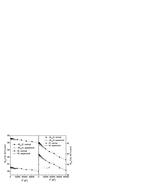
Figure 3: Comparison of normal and superconducting state for the optical sum and the kinetic energy. The left hand frame applies to Model A of Table 1 and $\omega_{SF}=82\,$meV and the right hand frame is for the band structure Model B of Table 1 and $\omega_{SF}=10\,$meV. The dotted line in this frame shows a $T^{2}$ law extrapolation of the normal state data for $T>T_{c}$ to zero temperature. Adapted from Ref. ref40, .

which gives the deviation from the $T^{2}$ law noted above is the small value of the spin fluctuation frequency $\omega_{SF}=10\,$meV used in Model B. This implies that the thermally activated scattering is larger in this model than it is for Model A. Later, when we consider simpler versions of our interaction model, we will return to this issue where it will become much easier to trace these dependencies.

In Fig. 3 we compare normal and superconducting state for the two models of Table 1. We see that both KE and OS (open squares and up triangles, respectively) fall below their normal state values (solid squares and up triangles, respectively) at the same temperature. This corresponds to an increase in KE as the superconducting state is entered. The changes are small in all cases. The KE in meV has increased by 0.2% for Model A and by 0.77% in Model B between superconducting and normal state at $T=0$. For the OS the differences are 0.22% and 0.6%, respectively, very comparable to what is found for the KE but not identical. We note that in the NAFFL model once the susceptibility (21) is specified, superconducting solutions with $d$-wave symmetry result. These are not put in by hand as to symmetry or functional form. The gap involves a harmonic $[\cos(ak_{x})-\cos(ak_{y})]$ as well as many of the higher harmonics consistent with the $d_{x^{2}-y^{2}}$ irreducible representation of the symmetry group for the square CuO₂ lattice. The solutions are far from simple BCS. In $d$-wave BCS an ansatz on the pairing potential $V_{{\bf k},{\bf k}^{\prime}}$ is made that it have the form $\eta_{\bf k}V\eta_{{\bf k}^{\prime}}$ with $\eta_{\bf k}\sim[\cos(ak_{x})-\cos(ak_{y})]$. This leads to a $d$-wave gap consisting of the lowest harmonic only. Early solutionsref38 based on Model A with $\omega_{SF}=7.76\,$meV showed that the gap had maximum amplitude at the $X$-point $(\pi,0)$ of the two dimensional CuO₂ Brillouin zone with $\Delta_{max}^{BZ}=33\,$meV. On the other hand the maximum gap on the Fermi surface was $\Delta_{max}^{FS}=27\,$meV at $T=20\,$K far below its BZ maximum. The value of $2\Delta_{max}^{FS}/(k_{B}T_{c})=6.27$ is quite different from the BCS value of 4.28. Also shown on the right hand panel is a dotted straight line which indicates the least squares fit extrapolation of the normal state data to zero temperature from $T>T_{c}$. It represents a $T^{2}$ law. It is important to notice, for later reference, that both, the superconducting as well as normal state $W$ data are above this dotted line for all temperatures $T<T_{c}$.

II.4 The Hubbard Model and Dynamical Mean Field

Another approach used to treat strongly correlated systems such as the cuprates is Dynamical Mean Field Theory (DMFT).ref41 The approach is numerical and based on the Hubbard model with hopping $t$, onsite Coulomb repulsion $U$, and chemical potential $\mu$. The half bandwidth $D=8\,t$ is taken to be $1.2\,$eV in what follows with $U=3D/2=12\,t$, so that the antiferromagnetic super exchange $J=4\,t^{2}/U\simeq 100\,$meV. For large values of $4U/D$ at half filling the system is a Mott insulator. Away from half filling, the weight of the quasiparticle peak at the Fermi level denoted by $Z$ and related to the self energy $\Sigma(\omega)$ by

$$Z=\left[1-\left.\frac{\partial\Sigma(\omega)}{\partial\omega}\right|_{\omega=0}\right]^{-1}$$

is non zero but small and is a measure of the metalicity.

The Hamiltonian used has the form

$$H=-t\sum\limits_{\langle ij\rangle\sigma}c^{\dagger}_{i\sigma}c_{j\sigma}+U\sum\limits_{i}n_{i\uparrow}n_{j\downarrow}-\mu\sum\limits_{i}\left(n_{i\uparrow}+n_{i\downarrow}\right),$$ (23)

where $\sigma$ is spin $\uparrow$, $\downarrow$, $c_{i\sigma}$ ($c^{\dagger}_{i\sigma}$) are annihilation (creation) operators for fermions of spin $\sigma$ on site $i$, $n_{i\sigma}=c^{\dagger}_{i\sigma}c_{i\sigma}$, and the sum $\langle ij\rangle$

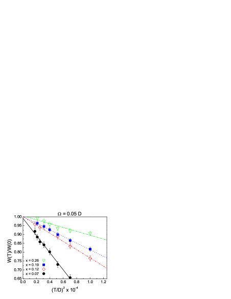
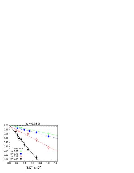
Figure 4: (Color online) $W(\Omega,T)$ normalized to its $T=0$ value as a function of $T^{2}$ for the Hubbard model, for $\Omega=0.05\,D$ (top frame) and $\Omega=0.75\,D$ (bottom frame). Symbols are the results of the DMFT calculations; lines are best fits to them. The various symbols give four dopings $(x)$. Adapted from Ref. ref42, .

is restricted to nearest neighbors only. In DMFT the full many body system with strong interactions is modeled as a single site problem with relevant interactions between, say, two electrons at that site plus coupling to a bath which represents on average the remaining degrees of freedom. The bath and local problem is to be solved for in a self consistent way. The method is now well developed and has proved its ability to simultaneously describe low and high energy features in Mott systems. Toschi et al.ref42 have calculated the real part of the optical conductivity in this model and obtained the results

Figure 5: The relative variation of spectral weight between the lowest $T$ and $300\,$K as a function of doping $x$ for various cuprates (full symbols) is compared with DMFT calculations (open squares) and with the predictions of non interacting models [tight binding model (solid line), constant density of states approximation (dashed line)]. The dotted line is a guide to the eye. The simple inclusion of correlation effects allows one to reproduce the observed absolute values with no need of fitting parameters. Data for LSCO are obtained from Refs. ref43, and ref44, , and for BSCCO from Refs. ref45, ; ref46, ; ref47, (BSCCO₁) and from Ref. ref48, (BSCCO₂). Adapted from Ref. ref42, .

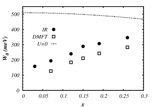
Figure 6: The $T=0$ spectral weight $W_{0}$ for $\Omega=0.75D$ as a function of doping $x$ for the Hubbard model (open squares) and the experimental observation of Lucarelli et al. Ref. ref44, (solid circles) obtained by integrating data on $\sigma_{1}(\omega)$ for LSCO. The dotted curve is for reference and gives results for $U=0$ (no correlations included). Adapted by A. Toschi from Ref. ref42, .

shown in Fig. 4 for various values of the doping $x$ as indicated in the figure which gives $W(\Omega,T)/W(\Omega,T=0)$ as a function of $(2T/D)^{2}$. The left hand frame employs a cutoff $\Omega$ in Eq. (1) of $0.05D$ while the right hand frame is for $\Omega=0.75D$. All curves appear to follow a $T^{2}$ behavior and the slope of these lines becomes smaller with increasing $\Omega$. A comparison of their DMFT results with experiment is also offered by the same authors and we reproduce it in Fig. 5 where we show the difference $\Delta W\equiv W(T=0)-W(T=300\,{\rm K})$ for $\Omega=1.5\,D$ renormalized to $W_{0}=W(T=0)$ denoted by $\Delta W/W_{0}$ on the figure as a function of doping $x$ (open squares).

Experimental results are for La_2-xSr_xCuO₄ (LSCO, solid circles), Refs. ref43, and ref44, , and Bi₂Sr₂CaCu₂O_8+x. Solid squares are from Refs. ref45, ; ref46, ; ref47, (BSCCO₁) and solid triangles from Ref. ref48, (BSCCO₂). Also shown for comparison are results for tight binding with no interactions (solid line) and in a constant density of states approximation (dashed line). It is clear that correlations dominate the observed change in $W$ between zero and $300\,$K to its $T=0$ value. DMFT provides a reasonable fit to the data while tight binding fails badly, giving values that are too small.

In Fig. 6 DMFT results (open squares) as a function of doping $x$ are compared with the experimental results (sold circles) of Lucarelli et al.ref44 for the optical sum of LSCO at $T=0$. The theory reproduces well the doping dependence of $W_{0}\equiv W(\Omega=0.75D,0)$. While the absolute value of $W_{0}$ is somewhat underestimated its large decrease as the Mott transition is approached is well captured by the model calculations. Also shown on the same figure (dotted line) are results obtained in the limit $U=0$ (no Hubbard $U$). We see that in this case the observed trend with doping is not reproduced and $W_{0}$ is much too large, particularly at small dopings indicating, as expected, that near the Mott transition $W_{0}$ goes like $x$ rather than $1-x$. Finally, we note that the inclusion of $U$ (correlation effects) reduces $W_{0}$ just as we have seen in the NAFFL model. We note, however, that this model is not well suited to describe doping differences because the phenomenological spin susceptibility (19) really needs to be fixed to some experimental observation at each doping level, particularly as the Mott transition is approached.

One thing to note about the DMFT results shown in Fig. 4 is that even for the smaller value of the cutoff $\Omega$ on the OS, a $T^{2}$ behavior is observed at least for the limited data available in the figure. By contrast, we have seen in the NAFFL calculations of Figs. 2 and 3 that deviations from $T^{2}$ can occur when the characteristic spin fluctuation energy $\omega_{SF}$ is small even when the sum is taken over the entire band, i.e.: $\Omega$ is large enough to include all contributions. Thus, the two calculations differ in this important point. We will see later that there is no guarantee that a given model for the interactions should always give a $T^{2}$ law.

To end we mention related Hubbard model work by Maier et al.ref89c They work directly with the KE rather than with the conductivity as did Toschi et al.ref42 and use the dynamical cluster approximation (DCA). They present results in both normal and superconducting state for two doping levels, namely $x=0.05$ and $x=0.2$. In both cases the KE is found to decrease with decreasing temperature even in the superconducting state and this decrease, in fact, drives superconductivity. The changes are of order a few percent at most.

As we have been so far mainly interested in the normal state we postpone further discussion of this work to a later section which deals explicitly with the superconducting state. We will also describe the recent work of Haule and Kotliarref89b which deals with the $t$-$J$ model (see Sec. IV).

III The effect of interactions in isotropic boson exchange models

III.1 Self Energy in Finite Bands

Recent studies of finite band effects have revealed that the self energy due to impurities or to interaction with bosons is profoundly changed by the application of a cutoff $\pm D/2$ in a half filled band.ref54 ; ref55 ; ref56 ; ref57 ; ref58 ; ref59 ; ref62 In a finite band, the normal state self energy due to the electron-phonon (or some other boson) interaction is given by

$$\Sigma(z) = T\sum\limits_{m}\lambda(z-i\omega_{m})\eta(i\omega_{m})$$

$$+\int\limits_{0}^{\infty}\!d\nu\,\alpha^{2}F(z)\left\{[f(T,\nu-z)+n(T,\nu)]\right.$$

$$\left.\times\eta(z-\nu)+[f(T,\nu+z)+n(T,\nu)]\eta(z+\nu)\right\},$$

in the mixed representation of Marsiglio et al.ref60 Here,

$$\lambda(z)=\int\limits_{0}^{\infty}\!d\nu\alpha^{2}F(\nu)\frac{2\nu}{\nu^{2}-z^{2}}$$ (24b)

and

$$\eta(z)=\int\limits_{-\infty}^{\infty}\!d\epsilon\,\frac{N_{0}(\epsilon)}{N_{0}(0)}\frac{1}{z-\epsilon-\Sigma(z)}.$$ (24c)

These equations need to be solved self consistently as $\Sigma(z)$ itself depends on itself through Eq. (24c). Here $z$ is a complex variable, $n(T,\nu)$ is the Bose thermal factor, $\alpha^{2}F(z)$ the electron-phonon spectral density and $N_{0}(\epsilon)/N_{0}(0)$ the normalized bare electronic density of states taken here to be constant and confined to $[-D/2,D/2]$. This provides a band cutoff in $\eta(z)$ of Eq. (24c) and makes Eq. (LABEL:eq:23) self consistent. These equations are also given by Karakozov and Maksimovref53 where they are written either in pure Matsubara notation or fully on the real frequency axis rather than in the mixed notation of Eqs. (24) which includes both versions, Matsubara and real axis. We have found the mixed notation more convenient for numerical work. For coupling to a single Einstein boson mode $\alpha^{2}F(\omega)=a\delta(\omega-\Omega_{E})$ where $\Omega_{E}$ and $a$ are taken in units of $D/2$. The electron mass renormalization is given by $\lambda=2a/\Omega_{E}$ which is dimensionless. For an infinite band at $T=0$ we recover from Eqs. (24) the very familiar resultref62

$$\Sigma_{1}(\omega)=a\ln\left|\frac{\omega-\Omega_{E}}{\omega+\Omega_{E}}\right|,$$ (25)

and

$$\Sigma_{2}(\omega)=-\pi a\theta\left(|\omega|-\Omega_{E}\right),$$ (26)

where $\theta(x)$ is the theta function equal to one for $x>0$ and zero otherwise. For positive values of $\omega$ the real part $\Sigma_{1}(\omega)\leq 0$ and approaches zero as $\omega\gg\Omega_{E}$. The imaginary part $\Sigma_{2}(\omega)$ is zero till $|\omega|=\Omega_{E}$ at which point it jumps to a value of $\pi a$ and then stays constant. Finite band effects change this behavior radically.

In Fig. 7 we show results of Knigavko and Carbotteref58 for minus the imaginary part $[-\Sigma_{2}(\omega)]$ of the self energy in frame (a) and its real part $[\Sigma_{1}(\omega)]$ in frame (b) for

Figure 7: Evolution of the self energy vs frequency dependence with temperature for the Einstein spectrum with $a=0.1$ and $\Omega_{E}=0.1$ $(\lambda=2)$. Frame (a) is for minus the imaginary part, $-\Sigma_{2}(\omega)$, while frame (b) is for the real part, $\Sigma_{1}(\omega)$. In each frame the different curves correspond to temperatures $t\equiv 2T/D=0.1$ (dash-dotted line), 0.05 (dotted line), 0.01 (dashed line), 0.001. All energies are in units of $D/2$. Adapted from Ref. ref58, .

coupling to a single Einstein phonon at $\Omega_{E}=0.1$ with mass enhancement parameter $\lambda=2$ for different temperatures, all in units of $D/2$. The temperatures are as given in the figure caption. The sharper curves correspond to the lower temperatures. For $T=0$, $\Sigma_{1}(\omega)$ has a logarithmic like singularity at $\omega=\Omega_{E}$ as in the infinite band case of Eq. (25) but now, rather than remain negative as it goes towards zero for $\omega\gg\Omega_{E}$, $\Sigma_{1}(\omega)$ crosses the $\omega$-axis and takes on large positive values before dropping towards zero from above. Equally different from the infinite band case, $-\Sigma_{2}(\omega)$ is not a constant equal to $\pi a$ [see Eq. (26)] above $\omega>\Omega_{E}$ but rather drops as we approach the bare band edge at $\omega=1.0$ after which it becomes small for $\omega\stackrel{{\scriptstyle>}}{{\sim}}1.5$ which is where the renormalized density of states $\tilde{N}(\omega)$ also becomes small. For further discussion of finite band features we refer the reader to Refs. ref54, to ref62, as well as to Ref. ref53, where a somewhat different density of states model is used but this does not change the qualitative behavior of the self energy seen in Fig. 7. An advantage of Karakozov and Maksimov’s choice of DOS, however, is that they can get a simple analytic expression for the self energy which they also show to be accurate by comparing with numerical results based on the full Eliashberg equations.

We return next to the OS of Eq. (10). One can get insight into the relative importance of the temperature dependence carried by the thermal factor $f(T,\omega)$ in $\bar{W}(T)$ and the temperature

Figure 8: The probability of occupation $n(\epsilon)$ of a state of energy $\epsilon$ vs normalized energy $2\epsilon/D$. (a) The results for the case when only the temperature dependence of the self energy is included. The normalized temperatures are $t\equiv 2T/D=0.0$ (solid line), 0.01 (dashed line), 0.03 (dotted line), and 0.05 (dash-dotted line). (b) Comparison of the results when the complete temperature dependence of $n(\epsilon)$ [see Eq. (10)] is accounted for (solid lines) with the case presented in frame (a). The normalized temperatures are $t=0.01$ (dashed line) and 0.05 (dash-dotted line). (All energies are in units of $D/2$.) A constant density of states model with cutoff $\pm D/2$ is used. Adapted from Ref. ref49, .

dependence solely due to the interactions in $A(\epsilon,\omega)$. In Fig. 8 we show results obtained by Knigavko et al.ref49 for $n(\epsilon)$, Eq. (5). Frame (a) shows $n(\epsilon)$ vs the renormalized energy $2\epsilon/D$ for four values of reduced temperatures $t=2T/D$, namely 0.0 (solid line), 0.01 (dashed line), 0.03 (dotted line), and 0.05 (dash-dotted line) when only the temperature dependence in $A(\epsilon,\omega)$ is included, i.e.: the $f(T,\omega)$ factor in $n(\epsilon)$ was excluded. Here we have considered coupling to a single phonon of energy $\Omega_{E}=0.04$ with mass enhancement $\lambda=1$. It is clear that considerable temperature dependence comes from this source alone and will influence the temperature dependence of the OS. In frame (b) of Fig. 8 we show results (solid curves) when both sources of $T$ dependence in $n(\epsilon)$ are included and compare with the two equivalent curves of frame (a) for $t=0.01$ (dashed line) and 0.05 (dash-dotted line). It is clear from these figures that the temperature dependence of the self energy is always important in determining the probability of occupation, $n(\epsilon)$, of a state of energy $\epsilon$ and hence the OS’s $T$ dependence.

III.2 Results for a delta-function boson model

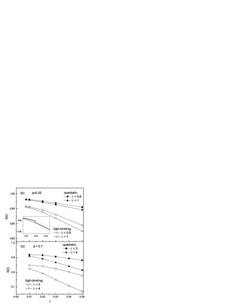
Figure 9: The variation of the optical sum $S$ vs reduced temperature $t=2T/D$ for the interaction strengths (a) $a=0.02$ and (b) $a=0.1$. The results are for both the quadratic (solid symbols) and tight binding (open symbols) bands, as indicated. In the top frame the mass enhancement factor $\lambda=0.8$ (squares) and $\lambda=1$ (triangles), while in the bottom frame $\lambda=2$ (squares) and $\lambda=4$ (triangles). The inset in the top frame illustrates the behavior of the optical sum during a sudden “undressing transition” at $t_{undress}=0.02$ with 20% hardening of the normalized boson frequency $\Omega$ and a corresponding reduction of the mass enhancement factor from $\lambda=1.0$ to 0.8. Adapted from Ref. ref49, .

Results for the OS normalized by a factor of $\hbar^{2}/(2m_{b})$ for the tight binding case (10) and by $\hbar^{2}\,n/m$ for the quadratic dispersion, both denoted by $S(t)$, are given in Fig. 9 reproduced from Knigavko et al.ref49 The parameters are as shown on the figure and given in the caption. The top frame is for $a=0.02$ and the bottom frame for $a=0.1$. The former corresponds to a conventional metal while the latter may be more characteristic of the cuprates. Two representative values of the boson energy $\Omega_{E}$ have been chosen to get $\lambda=0.8$ (squares) and 1.0 (triangles) in the top frame and $\lambda=2$ (squares) and $\lambda=4$ (triangles) in the bottom frame. Both tight binding (open symbols) and quadratic (solid symbols) dispersion relations are considered. It is quite clear from these results that the temperature dependence of the OS needs not be quadratic and depends on the size of the coupling to the phonons ($\lambda$ value) and also on the dispersion relation used to describe the electron dynamics. An important observation for what will follow is contained in the inset of the top frame of Fig. 9. The heavy solid line follows the temperature evolution of the OS when a sharp “undressing” transition is assumed to take place at $t=0.02$ where a 20% hardening of the phonon spectrum occurs. This corresponds to a shift in the mass enhancement parameter from $\lambda=1$ to 0.8. Such a hardening of the phonon energy leads to an increase in the OS corresponding to a decrease in the KE of the charge carriers.ref49

III.3 Results for an MMP spin fluctuation model

The delta function spectra used in the work of Knigavko et al.ref49 while giving us insight into the mechanism that leads to temperature dependences in the OS is not realistic for the cuprates. If one wishes to remain within the framework of a boson exchange mechanism one should at the very least choose a different form for $\alpha^{2}F(\omega)$. For spin fluctuation exchange a much used choice is the MMP model of Millis et al.ref37 ; ref61 ; ref63 In its simplest form $\alpha^{2}F(\omega)$ which will now be denoted $I^{2}\chi(\omega)$ is taken as

$$I^{2}\chi(\omega)=I^{2}\frac{\omega/\omega_{SF}}{1+(\omega/\omega_{SF})^{2}},$$ (27)

with $I$ a coupling between charge carriers and spin susceptibility and $\omega_{SF}$ a spin fluctuation frequency. Here, the coupling $I$ is adjusted to get a superconducting transition temperature $T_{c}$ of

Figure 10: Top frame: minus the imaginary part of the carrier self energy $-\Sigma_{2}(\omega,T)$ vs $\omega$ at the various temperatures shown. Middle frame: minus the real part of the carrier self energy $\Sigma_{1}(\omega,T)$ vs $\omega$. Bottom frame: the function $h(T,-\omega)$ of Eq. (11) vs $\omega$. The calculation is for an MMP model, Eq. (27), with $\omega_{SF}=20\,$meV, $I^{2}=0.82$, and $D=800\,$meV.

$100\,$K when used in the corresponding Eliashberg equations generalized for a $d$-wave gap symmetry. In this section we concentrate on the normal state only. Thus, Eqs. (24) apply with $\alpha^{2}F(\omega)$ replaced by Eq. (27). Results for a case with $\omega_{SF}=20\,$meV, $I^{2}=0.82$, and $D/2=400\,$meV are shown in Fig. 10 which has three frames. In the top frame we show $-\Sigma_{2}(T,\omega)$ for four temperatures as labeled, in the center frame $\Sigma_{1}(T,\omega)$, and in the bottom frame $h(T,-\omega)$ vs $\omega$. It is clear that both real and imaginary part of $\Sigma(T,\omega)$ have important $T$ dependencies which get reflected in $h(T,\omega)$ and consequently in the OS given by Eq. (10) and more approximately by Eq. (12) with

Figure 11: The reduced optical sum $S(T)$ according to Eq. (28) vs temperature $(T)$ squared. The left hand frame is for an MMP model (27) with $\omega_{SF}=20\,$meV and $I^{2}=0.82$ while the right hand frame is for $\omega_{SF}=82\,$meV and $I^{2}=0.655$.

the last term dropped. In this instance it is simply the area under $h(T,\omega)$ for negative $\omega$ that determines the OS while in Eq. (10) it is its overlap with the Fermi distribution and this has an additional temperature dependence due to $f(T,\omega)$ but it is small. Results for

$$S(T)=2\bar{W}(T)\frac{m_{b}}{\hbar^{2}}$$ (28)

are shown in Fig. 11 which has two frames. In the left hand frame we show results for $S(T)$ vs $T^{2}$ up to $40000\,$K² for our MMP model with $\omega_{SF}=20\,$meV and $I^{2}=0.82$ while in the right hand frame $\omega_{SF}$ is increased to $82\,$meV with $I^{2}=0.655$. In both cases the full band width $D$ ranges over 2500 (dashed line), 800 (solid line), and $500\,$meV (dash-dotted line). It is clear that decreasing $D$ reduces the value of $S(T=0)$ and gives a stronger $T$ dependence which, nevertheless, remains near a $T^{2}$ behavior for the right hand frame but not in the left hand frame. These results are in qualitative agreement with those shown in the previous section, Figs. 1 and 3 obtained in a tight binding model with a k-point sampling method of the Brillouin zone and the full momentum dependent Eliashberg equations (20). Also shown in both frames as a dotted curve for the case $D=800\,$meV are straight lines which allow us to judge better the deviations from a $T^{2}$ law at small $T$ in the curves of the left hand frame. For the right hand frame there is little deviation. Note that both these behaviors are completely consistent with numerical results of Fig. 3 and show that the upward deviation at small $T$ of the solid curve as compared with the dotted $(T^{2})$ is a robust result not dependent on the model used, provided that the spin fluctuation frequency is small. Note also that Eq. (10) includes $T$ variations in $h(T,\omega)$ as well as the thermal factor $f(T,\omega)$, but this latter factor can be neglected. The differences are very small confirming our previous claim that the temperature dependence in $S(T)$ is mainly due to variations in the interaction term at least for these cases. Finally, we stress again that the $T^{2}$ law found in the DMFT calculations for the Hubbard model and often confirmed in experiments also arises in the NAFFL model with an MMP interaction provided the spin fluctuation energy is fairly large and $D$ not too small. In principle, however, there is no fundamental reason for an exact $T^{2}$ law. The actual $T$ dependence of $S(T)$ comes from the $T$ dependence of the area under the curves for $h(T,-\omega)$ (bottom frame of Fig. 10). We see that these curves change most at small $\omega$ as $T$ is increased but there are also important changes at large $\omega$ and we are sampling an average of these changes. Nevertheless, the $\omega$ dependence of $\alpha^{2}F(\omega)$ or $I^{2}\chi(\omega)$ at low energies $\omega$ will determine most strongly the temperature dependence of $h(T,-\omega)$ at those energies and, thus, plays an important role in the temperature dependence of $S(T)$. However, even at higher energies there is still significant $T$ dependence in $h(T,-\omega)$.

III.4 The non $T^{2}$ temperature dependence of the optical sum

Benfatto et al.ref52 have reconsidered the effect of

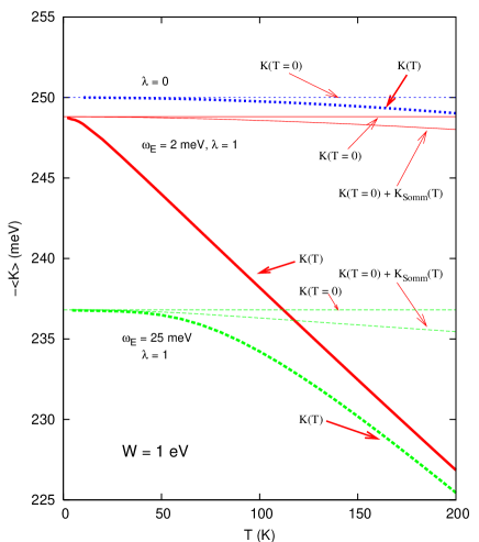
Figure 12: (Color online) The negative of the KE, $-\langle K\rangle$, vs temperature showing the breakdown for the various contributions. The solid curves are for a small boson frequency $\omega_{E}=2\,$meV with $\lambda=1$. The two thin lines show how the zero temperature value is modified by the Sommerfeld term by a very small amount. A similar size contribution (actually a bit larger) is illustrated for the noninteracting case by dotted curves, where only the Sommerfeld term is responsible for the temperature variation. Finally, for higher boson frequencies, the dashed curves illustrate the amount of temperature variation due to the Sommerfeld term compared with the rest. The band width $W\equiv D=1\,$eV. Adapted from Ref. ref52, .

interaction on the temperature dependence of $S(T)$ with an aim at providing simple analytic expressions that would help trace more directly the dependence on the interactions. In Fig. 12 we reproduce some of their results for the temperature dependence of the negative of the KE, $-\langle K\rangle\equiv K(T)$, in meV. The two dotted lines at the top of the graph represent the noninteracting case $(\lambda=0)$ and are for reference. As expected, there is little difference between $K(T)$ and its zero temperature value $K(T=0)$. The three solid curves are for a system with coupling to a boson of frequency $\omega_{E}=2\,$meV and $\lambda=1$. We see that $K(T=0)$ and $K(T=0)+K_{\rm Somm}(T)$, the Sommerfeld contribution, are not significantly different. Thus, $K_{\rm Somm}(T)$ is not the important contribution to the temperature dependence of the complete KE [heavy solid line, denoted $K(T)$] which develops a linear temperature dependence for $T\sim 20\,$K. The same holds for the case $\omega_{E}=25\,$meV (three dashed curves) but the variation in $T$ of $K(T)$ in this case is less pronounced and closer to a $T^{2}$ law as was found for the MMP spectrum. The band width in all three cases was $W\equiv D=1\,$eV. Benfatto et al.ref52 trace these $T$ dependences in detail using analytic as well as numerical techniques. They concluded that both the real and imaginary parts of $\Sigma$ contribute. Karakozov and Maksimovref53 also find deviations from a $T^{2}$ law and provide an approximate analytic formula for these deviations in a particular case. For different models of $\alpha^{2}F(\omega)$ other $T$ dependencies are possible. This means that in principle one can learn about some features of this underlying $\alpha^{2}F(\omega)$ from a study of the temperature dependence of the OS, but the correspondence is not necessarily simple or unique. On the other hand, a complete study of the temperature and frequency dependence of the optical self energyref64 as is now done routinely, provides much more detailed information than does the OS. Recall that $h(T,\omega)$ is dependent on an average over the real and imaginary part of $\Sigma$, the quasiparticle self energy. This information is accessible directly from angular resolved photoemission spectroscopy (ARPES) at each point in the Brillouin zone separately.

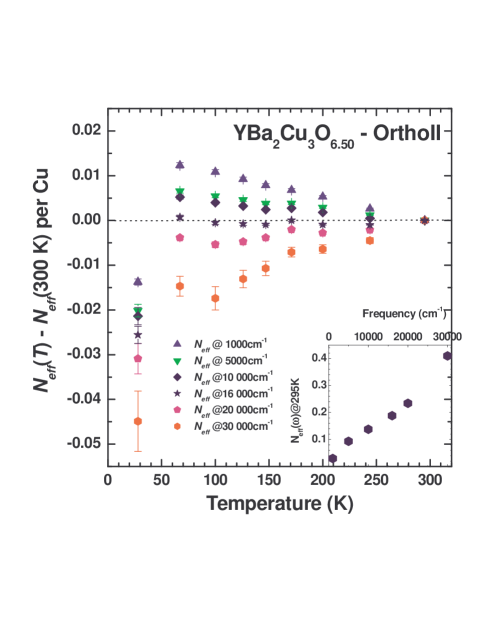
Figure 13: (Color online) The partial spectral weight integrated up to various frequencies as a function of temperature. Below $16\,000\,$cm^-1 there is an increase in spectral weight as the temperature is lowered signaling a line narrowing on this frequency scale. Below $T_{c}$ there is strong loss of spectral weight to the superconducting condensate. There is no evidence of any precursors to superconductivity at $67\,$K. In the inset we show $N_{eff}(\omega)$ at $295\,$K. Adapted from Ref. ref64, .

While many experiments give a $T^{2}$ dependence in the normal state within the precision of measurement there is some evidence for other dependences in the cuprates. In Fig. 13 we reproduce data from the paper of Hwang et al.ref64 for the partial sum to $\omega_{c}$ in units of carriers per Cu atom denoted by $N_{eff}(T)$. What is shown is the difference $N_{eff}(T)-N_{eff}(300\,{\rm K})$ as a function of temperature $T$ to $300\,$K. The data is for underdoped YBa₂Cu₃O_6.50 (YBCO_6.50) Ortho II material of high quality and purity. There are 5 values of $\omega_{c}$, namely 1000, 5000, $10\,000$, $16\,000$, and $20\,000\,$cm^-1. It is clear that the temperature dependence of $N_{eff}(T)$ is not necessarily quadratic in $T$ for the partial sums and also for the case most relevant for our discussions with $\omega_{c}=16\,000\,$cm^-1. These samples are, however, underdoped and a pseudogap is involved which could have some effect on the temperature dependence of the OS as we will discuss later within a phase fluctuation model for the pseudogap and alternatively a $D$-density wave model.

IV The Optical Sum in the Superconducting State

IV.1 Superconducting optical sum including of inelastic scattering collapse

Figure 14: Experimental values of the $ab$-plane spectral function $\rho_{L}$ defined in Eq. (29). Adapted from Ref. ref34, .

Next we return to a more detailed look at the superconducting state. In Fig. 14 we reproduce the original results of Molegraaf et al.ref48 for two samples of BSCCO as they were presented by van der Marel et al.ref34 The top frame is for optimally doped and the bottom frame for an underdoped sample. What is shown is

$$\rho_{L}\equiv C\frac{\hbar^{2}}{\pi e^{2}}\int\limits_{-\Omega}^{\Omega}\!d\omega\,\Re{\rm e}[\sigma(\omega)]$$ (29)

in meV with $C$ a constant to be specified shortly. It is striking that in these two samples the OS appears to increase faster in the superconducting state than in the underlying normal state extrapolated to low temperatures (dotted line). This was interpreted by Molegraaf et al.ref48 as indicating a decrease in KE in the superconducting state as compared with the underlying normal state which also shows a decrease in KE as $T\to 0$ but by less than in the superconducting state. This behavior clearly goes beyond ordinary BCS theory and also Eliashberg theory as formulated for phonons.

There remains some controversy about the interpretation of such data with some authors finding the opposite effect.ref65 We will not go into these details here but refer the reader to some relevant literatureref65 ; ref66 ; ref67 and note that Santander-Syroref47 confirm the basic results of Molegraaf et al.ref48 See also the recent work of Carbone et al.ref33a

We have already seen in Fig. 9 [inset in frame (a)] for the normal state, that undressing effects associated with a hardening of the phonon spectra at a particular onset temperature can give an OS curve that behaves very much like those seen in Fig. 14. While in principle phonon frequencies can shift as a result of the onset of superconductivity these effects are small and usually negligible. For an electronic mechanism, however, we have already discussed in the introduction the idea of the collapse of the inelastic scattering as superconductivity sets in which leads directly to a peak in the real part of the microwave conductivity at some intermediate temperature below $T_{c}$. Within a spin fluctuation mechanism this translates into a hardening of the spin fluctuation spectrum and the modification of $I^{2}\chi(\omega)$ of Eq. (27) as the $d$-wave superconducting gap opens. An analysis of the optical scattering rates in YBCO_6.95 by Carbotte et al.ref68 showed that

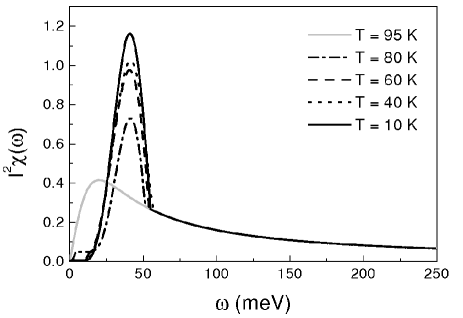
Figure 15: The charge carrier-spin spectral density $I^{2}\chi(\omega)$ determined from optical scattering data of YBCO_6.95 at various temperatures. Solid gray curve $T=90\,$K, dash-dotted $T=80\,$K, dashed $T=60\,$K, dotted $T=40\,$K, and black solid $T=10\,$K. Note the growth in strength of the $41\,$meV optical resonance as the temperature is lowered. Adapted from Ref. ref70, .

there is a reduction in $I^{2}\chi(\omega)$ at small $\omega$ as the temperature is reduced. Results obtained by Schachinger et al.ref69 ; ref70 for the temperature evolution of $I^{2}\chi(\omega)$ in YBCO_6.95 are reproduced in Fig. 15. We see a reduction in spectral weight at low $\omega$ as well as the growth of an optical resonance at $41\,$meV, the energy of the spin one resonance seen in neutron scattering.ref71 When these spectra are used in a

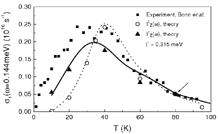
Figure 16: Temperature dependence of the conductivity $\sigma_{1}(\omega)$ at microwave frequency $\omega=0.144\,$meV in YBCO_6.95. The open circles are results based on our model spectral density (see Fig. 15) obtained from inversion of optical conductivity data and the dashed line is based on an MMP model with low frequency cutoff. The solid triangles include impurities with the solid line from Ref. ref74, . The solid squares represent experimental data by Bonn et al.ref75 Adapted from Ref. ref69, .

generalization of the ordinary Eliashberg equations that includes the possibility of $d$-wave symmetry with gap $\Delta(\phi)=\Delta_{0}\cos(2\phi)$ where $\phi$ is an angle on the Fermi surface taken to be cylindrical, Schachinger and Carbotte,ref70 ; ref72 find excellent agreement for the microwave data of Hosseini et al.ref73 taken at five different microwave frequencies on high quality samples of YBCO_6.99. In Fig. 16, reproduced from Ref. ref69, , we show older results obtained by Bonn et al.ref75 fit by Schachinger et al.ref74 by simply applying a low frequency cutoff to an MMP form.ref74 ; ref76 The data are given as the solid squares while the theoretical calculations without impurities (open circles and dashed line) and with impurities (solid triangles and solid line) are shown for comparison. Here $t^{+}$ gives the impurity scattering rate in Born approximation. Open circles and solid triangles are based on the spectra of Fig. 15 which include the $41\,$meV spin resonance. The dashed and solid lines are from earlier calculations based on an MMP spectrum with application of a low frequency cutoff without resonance.ref74 ; ref76 We see that such a procedure gives results that are very close to those based on the more exact results of Fig. 15.

Calculations in the model of Eqs. (20) of the OS and KE of optimally doped BSCCO have been carried out by Schachinger and Carbotteref40 who simulated

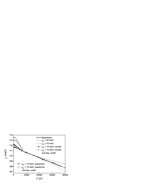
Figure 17: The optical sum of optimally doped BSCCO as a function of the square of the temperature for the band structure Model A of Table 1 with different values of $\omega_{SF}$. Also in one case a low frequency cutoff is applied to the spin susceptibility. Note the significance of the $T^{2}$-variation on the value of $\omega_{SF}$. The thick solid line represents experimental normal state data of Molegraaf et al.ref48 also shown in the top frame of Fig. 14. Adapted from Ref. ref40, .

the expected hardening of the spin fluctuation spectra in the superconducting state by applying a low frequency cutoff to the interaction of Eq. (21). This cutoff varies with temperature. It is zero at $T_{c}$ and has a maximum amplitude of $23\,$meV at $T=0$ with intensity changed according to a mean field BCS $d$-wave order parameter temperature dependence. Their results are shown in Fig. 17. The quantity $\rho_{L}$ according to Eq. (29) on the vertical axis is in meV and the horizontal scale is $T^{2}$ in K². The heavy solid line are normal state experimental data of Molegraaf et al.,ref48 also shown in the top frame of Fig. 14 of this review. The theoretical results for the OS are all based on Model A of Table 1 but were scaled upward by a factor [$C$ of Eq. (29)] of approximately two to fit the data. The spin fluctuation frequency $\omega_{SF}$ was also adjusted to improve the fit; $\omega_{SF}=13\,$meV is best. To reduce the discrepancy in absolute value of the OS the value of the nearest neighbor hopping parameter $t$ in our band structure model would need to be increased. This would, however, also decrease the sensitivity of the OS to temperature variations and so $\omega_{SF}$ would have to be adjusted downwards as well. Markiewicz et al.ref77 have suggested significantly larger values of nearest neighbor hopping $t$ for the bare band structure of BSCCO than used to fit ARPES data. As is well known, there can be a factor of two or more. We have used the dispersion relation of Table I of Ref. ref77, (specifically we used $t=360\,$meV, $t^{\prime}=-100\,$meV, and $\langle n\rangle=0.4$. We also included further neighbors, namely $t^{\prime\prime}=35\,$meV and $t^{\prime\prime\prime}=20\,$meV) and found a value of $W(T=0)$ of $230\,$meV well above the experimental value with $\omega_{SF}=8\,$meV giving the proper temperature dependence. It is clear that a value of $t$ intermediate between that of Markiewicz et al.ref77 and the one in Table 1 for Model A would be needed to get agreement with the OS data without any adjustment and a $\omega_{SF}$ value between 8 and $13\,$meV. Schachinger and Carbotteref40 did not attempt such a fit as their aim was not to fit any particular case but rather see how a low frequency cutoff applied to a spin fluctuation model changes the OS. The solid squares in Fig. 17 show the normal state results while the solid triangles are in the superconducting state. These are obtained without cutoff and so the KE has increased with respect to its normal state. The open squares and triangles show results for the same two cases but now the low frequency cutoff is applied to simulate the hardening of the spectrum as $T$ is reduced below $T_{c}$. We see a large decrease in KE as compared to the case without cutoff and the superconducting state would then show a decrease in KE as compared to the normal state without cutoff in agreement with the data of Fig. 14. It is the modification of the underlying interactions that have lead to this effect. It is clear that a modest hardening of the spectra consistent with the changes seen in the electron-boson spectral functions of Fig. 15 would be sufficient to explain the data in Fig. 14. Of course, in a complete theory as yet not attempted, it would be necessary to find an interaction which can give not only the correct OS but also the microwave peak and all the other properties of the superconducting state. Finally, we note that in Fig. 17 the OS shows a non $T^{2}$ behavior at low temperatures even without the low frequency cutoff which has the effect of making it more pronounced. If we did not have the normal state data below $T_{c}$ and simply extrapolated the normal state data above $T_{c}$ with a $T^{2}$ law to $T=0$ we would have to conclude that the OS is higher in the superconducting state than in the extrapolated “normal state” yet in this case the mechanism for pairing is not exotic in any way, i.e.: there is no low frequency cut off. (See also Fig. 3.) With the introduction of a low frequency cutoff this effect becomes even more pronounced and for the case shown the rise in the superconducting state is larger than seen in the experiments of Fig. 14. We caution the reader, however, that while this rise is seen by several experimental groups and is not controversial, its actual size is.

IV.2 The Temperature Dependent Scattering Time Model

Recently Marsiglioref90 has given calculations that provide support for the results of Fig. 17 using a related but much simpler model. He notes that in an infinite band for an elastic scattering rate $\Gamma$ the probability of occupation of the state $|{\bf k}\rangle$ at finite temperature is given by

$$n_{N}(\epsilon_{\bf k})=\frac{1}{2}-\frac{1}{\pi}\,\Im{\rm m}\psi\left(\frac{1}{2}+\frac{\Gamma}{4\pi T}+i\frac{\epsilon_{\bf k}}{2\pi T}\right)$$ (30)

for the normal state and, to a good approximation, by

$$n_{S}(\epsilon_{\bf k})=\frac{1}{2}-\frac{\epsilon_{\bf k}}{E_{\bf k}}\frac{1}{\pi}\Im{\rm m}\,\psi\left(\frac{1}{2}+\frac{\Gamma}{4\pi T}+i\frac{E_{\bf k}}{2\pi T}\right)$$ (31)

for the superconducting state with $E_{\bf k}=\sqrt{\epsilon_{\bf k}^{2}+\Delta_{\bf k}^{2}}$, with $\Delta_{\bf k}$ the superconducting gap and $\psi(z)$ is the digamma function. Note that at zero temperature

$$n_{S}(\epsilon_{\bf k})=\frac{1}{2}\left[1-\frac{\epsilon_{\bf k}}{E_{\bf k}}\frac{2}{\pi}\tan^{-1}\left(\frac{2E_{\bf k}}{\Gamma}\right)\right],$$ (32)

which, in the limit $\Gamma\to 0$, reduces to the well known expression $(1-\epsilon_{\bf k}/E_{\bf k})/2$, Eq. (15) introduced in Sec. II.2. It is clear from Eq. (32) that both, the appearance of a gap in $E_{\bf k}$ and the elastic scattering $\Gamma$ smear $n_{S}(\epsilon_{\bf k})$.

Figure 18: (Color online) Minus the kinetic energy, $-\langle T_{xx}\rangle$, vs temperature squared for various degrees of elastic scattering. Below $T_{c}$ we change the elastic scattering rate smoothly to zero [as $\Gamma_{0}(T/T_{c})^{4}$] as the temperature is lowered. Adapted from Ref. ref90,

From these expressions for $n(\epsilon_{\bf k})$ it is easy to work out the average KE which Marsiglio denotes by $-\langle T_{xx}\rangle$. He uses a tight binding band and a constant $\Gamma_{0}=1/\tau=0$, 2, 5, 10, and $15\,$meV from top to bottom in Fig. 18. For the superconducting state $\Gamma_{0}$ is changed to $\Gamma(T)$ with $\Gamma(T)=\Gamma_{0}(T/T_{c})^{4}$ which is observed in the work of Hosseini et al.ref73 This introduces phenomenologically the idea of the collapse of the scattering rate. We see in Fig. 18 that for $1/\tau=5\,$meV and larger the KE decreases below its normal state extrapolation as the system becomes superconducting. The change is of the order of a few percent for the largest $1/\tau$ considered and is large enough to explain the measured KE changes in the underdoped cuprates.

IV.3 The model of Norman and Pépin

The mechanism described above which leads to an OS increase as superconductivity sets in has some common elements with the ideas of Norman and Pépinref78 ; ref79 although there are also important differences. These authors use a less fundamental, more phenomenological approach based on ARPESref80 and optical conductivity data from which they construct directly a model for the self energy $\Sigma(\omega)$. For the normal state they begin with a constant, frequency independent scattering rate $\Gamma_{0}=\Im{\rm m}\Sigma(\omega)$ (taken to be of order $100\,$meV) to simulate the very broad (incoherent) line shapes seen in ARPES at the anti nodal point $(0,\pi)$. In the superconducting state a sharp coherence peak appears which signals increased coherence. To model this fact a low frequency cutoff $\omega_{0}$ is applied to the imaginary part of $\Sigma(\omega)$ making it zero for $\omega\leq\omega_{0}$ and $\Gamma_{0}$ above. The value of $\omega_{0}$ is chosen as the energy of the spectral dip feature seen in ARPES in the superconducting state. Here, as in the model described in Sec. IV.2, the underlying normal state on top of which superconductivity develops effectively has reduced scattering, i.e.: is more coherent which is a critical additional feature not contained in ordinary BCS and this leads to a reduction in KE and, consequently, in an increase of the OS. To arrive at their final estimates for the KE increase Norman and Pépin include further complications in their model such as the anisotropy observed in scattering ratesref81 ; ref82 ; ref83 ; ref84 ($\Gamma_{\bf k}$ instead of $\Gamma_{0}$)

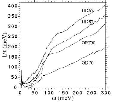
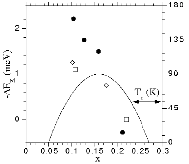
Figure 19: Top frame: The optical scattering rate $1/\tau(\omega)$ vs $\omega$ for various BSCCO samples from Ref. ref87, (OD overdoped, OPT optimal doped, UD underdoped). Bottom frame: Calculated sum rule violation $(-\Delta E_{K})$ vs doping $x$ (solid circles). The curve is $T_{c}$. Also shown in this frame are the experimental results (open squares from Ref. ref46, , open diamonds from Ref. ref48, ). The theoretical doping trend in (b) is due to the increasing offset in $1/\tau$ seen in (a). Adapted from Ref. ref78, .

going from anti nodal to nodal direction as well as an $\omega$ dependence (proportional to a momentum independent parameter $\alpha$) in the self energy modeled on the Marginal Fermi Liquid modelref85 ; ref86 with parameters determined from optical data on scattering rates. We reproduce in Fig. 19 their final estimates for the KE change $-\Delta E_{K}$ between superconducting and normal state. The left hand frame shows the optical scattering rate denoted $1/\tau(\omega)$ for four BSCCO samples from Puchkov et al.ref87 which they use to fit parameters. The right hand frame presents the results for the change in KE $(-\Delta E_{K})$ associated with the formation of the superconducting state in meV as a function of doping $x$. The solid circles give the theoretical results and the open squares and open diamonds experimental data from Santander-Syro et al.ref46 and Molegraaf et al.,ref48 respectively. The theoretical estimates are deemed reasonable but not accurate. On the overdoped side the OS behaves in a conventional fashion while for the underdoped side it is anomalous representing a lowering of KE as compared with what is expected in conventional BCS. Note that the lowest open square in this graph shown as being zero for the overdoped sample represents an early not very accurate estimate. In Ref. ref46, it is actually negative rather than zero bringing it closer in agreement with the lowest solid circle (theory). This point was further discussed by Deutscher et al.ref87a

IV.4 Additional data on kinetic energy changes

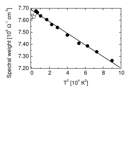
Figure 20: Spectral weight of the overdoped Bi2212 sample, integrated up to $1\,$eV, plotted vs $T^{2}$, from Ref. ref46, . Closed symbols: spectral weight in the normal state, open symbols: spectral weight in the superconducting state, including the weight of the superfluid. The errors in the relative variations of the spectral weight are of the size of the symbols. Adapted from Ref. ref87a, .

We reproduce in Fig. 20 the data of Santander-Syro et al.ref46 for their overdoped sample as presented by Deutscher et al.ref87a What is shown is the optical spectral weight in units $10^{6}\,\Omega^{-1}\,{\rm cm}^{-2}$ as a function of $T^{2}$. The solid circles are in the normal state and the open circles in the superconducting state below $T_{c}=63\,$K. A clear $T^{2}$ law is noted above $T_{c}$ and a reduction in spectral weight below, as expected in ordinary BCS theory. For the optimally doped sample

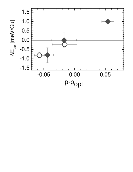
Figure 21: Change $\Delta E_{kin}$ of the KE, in meV per copper site vs the charge $p$ per copper site with respect to $p_{opt}$ [Eq. (33)] in BSCCO. Full diamonds: data from Ref. ref47, , high-frequency cutoff $1\,$eV. Open circles: data from Ref. ref48, , high frequency cutoff $1.25\,$eV. Error bars: vertical, uncertainties due to the extrapolation of the temperature dependence of the normal state spectral weight down to zero temperature; horizontal, uncertainties resulting from $T_{c}/T_{c,max}$ through Eq. (33). Deutscher et al.ref87a took $T_{c,max}=(83\pm 2)\,$K for films and $(91\pm 2)\,$K for crystals. Adapted from Ref. ref87a, .

(not shown) the normal state temperature dependence is closer to linear than quadratic and the underdoped sample shows a very flat region before entering the superconducting state. This demonstrates once more that there is as yet no strong consensus in the literature as to the $T$ dependence of the normal state. (Please see also Ref. ref89a, .) The same paper also analyses the data in terms of KE change for three samples UND70K, OPT80K, and OVR63K, as shown in Fig. 21 reproduced from Deutscher et al.ref87a The horizontal axis is $p-p_{opt}$ where $p$ is the charge per Cu atom related to $T_{c}$ by

$$\frac{T_{c}}{T_{c,opt}}=1-86.2\left(p-p_{opt}\right)^{2},$$ (33)

with $T_{c,opt}$ the maximum critical temperature for the Bi2212 series.ref89 What is clear from this figure is that there is a smooth crossover from standard behavior on the overdoped side to anomalous behavior on the underdoped side. The very recent data of Carbone et al.ref33a lends further support to this conclusion.

IV.5 Cluster dynamical mean field of the $t$–$J$ model

Recently Haule and Kotliarref89b calculated the optical conductivity of the $t$–$J$ model within a cluster DMFT (CDMFT). (Please see also earlier work by Maier et al.ref89c

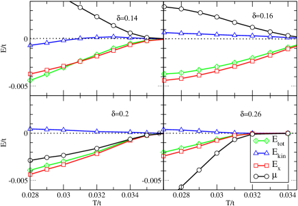
Figure 22: (Color online) The difference between the superconducting and normal state energies as a function of temperature. The following curves are shown: up-triangles - $E_{kin-S}-E_{kin-N}$; squares - $E_{x-S}-E_{x-N}$; diamonds - $E_{tot-S}-E_{tot-N}$; circles - $\mu_{S}-\mu_{N}$. Adapted from Ref. ref89b, .

based on the Hubbard model.) Haule and Kotliarref89b treat the temperature and doping dependence and address the issue of the change in KE of the holes when superconductivity sets in. They find, in agreement with experiment, that on the overdoped side the KE makes a negative contribution to the condensation energy as in conventional BCS theory but that there is a crossover to the opposite case on the underdoped side. This is shown in Fig. 22 reproduced from Ref. ref89b, . What is shown is the difference between the superconducting and normal state energies $(E)$ as a function of temperature, both in units of $t$ (nearest neighbor hopping). The up-triangles give the KE contribution $(E_{kin})$, the squares are the super exchange $(E_{x})$, and the diamonds the total energy $(E_{tot})$. We see a change in sign in the KE contribution upon condensation as we go from the overdoped to the underdoped regime. ($\delta$ denotes the doping.) These results contrast with earlier work of Maier et al.ref89c also based on the Hubbard model. There, the KE is found to be lower in the superconducting state than in the normal state for both values of doping presented, namely $\delta=0.05$ and $\delta=0.2$ (overdoped). In the underdoped case the potential energy increases slightly above its normal state value below $T=T_{c}$. For the overdoped case it does decrease very slightly but plays a much smaller role in the condensation than the corresponding drop in KE.

We end this section by mentioning two related worksref127 ; ref128 based on the negative $U$ Hubbard model which has been used successfully to describe the BCS - Bose Einstein (BE) crossover. Toschi et al.ref127 employ DMFT and Kyung et al.ref128 a cellular DMFT and obtain very similar results. Both normal and superconducting states are considered. Both groups find a change of sign in the KE difference between superconducting and

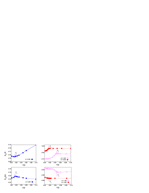
Figure 23: (Color online) Low-temperature behavior of the normalized kinetic energy $E_{\rm kin}/D$ (upper panels) and the normalized potential energy $E_{\rm pot}/|U|$ (lower panels) as a function of the normalized temperature $T/D$. Here $U$ is the Hubbard attraction. The critical temperature is marked by arrows. Adapted from Ref. ref127, .

normal state as one goes from underdoping (anomalous) to overdoping (conventional BCS behavior) as seen in Fig. 21. In Fig. 23 we reproduce from Ref. ref127, results for KE $(E_{\rm kin})$ in units of the band width $D$ vs the normalized temperature $T/D$ (upper frames) and for the potential energy $E_{\rm pot}$ in units of $|U|$ (lower frames). Three values of $U$ are considered, $U=0.4\,D$ in the left frames and $U=1.2\,D$ and $3.2\,D$ in the frames on the right. These values correspond to BCS, intermediate, and BE (Bose - Einstein) regimes, respectively. The frames on the left show conventional behavior with a small increase in KE in the superconducting state and a decrease in potential energy. On the other hand, in the frames on the right the KE decreases while the potential energy increases which is referred to as KE driven superconductivity.

V Models of the Pseudogap State

V.1 The Preformed Pair Model

Another model for superconductivity in the oxides is the preformed pair model.ref91 ; ref92 ; ref93 ; ref94 ; ref95 ; ref96 The idea is that the pairs form at a temperature $T^{\ast}$, the pseudogap formation temperature. The superconducting state emerges from the preformed pair state at a lower temperature $T_{c}$ when phase coherence sets in. The pseudogap regime is then due to superconducting phase fluctuations. In a recent paper Eckl et al.ref97 considered the effect of phase fluctuations on the OS, i.e.: the KE in the pseudogap regime. [See also the related work of Kopeć, Ref. ref97a, .] They start with a Hamiltonian which contains two terms, the KE

$$K=-t\sum\limits_{\langle ij\rangle\sigma}\left(c^{\dagger}_{i\sigma}c_{j\sigma}+c^{\dagger}_{j\sigma}c_{i\sigma}\right)$$ (34)

and a pairing term

$$-\frac{1}{4}\sum\limits_{i\delta}\left(\Delta_{i\delta}\left\langle\Delta^{\dagger}_{i\delta}\right\rangle+\Delta^{\dagger}_{i\delta}\left\langle\Delta_{i\delta}\right\rangle\right),$$ (35)

where $\delta$ connects the site $i$ to its nearest neighbors only and $\langle ij\rangle$, as before, is limited to nearest neighbors as well. Furthermore,

$$\Delta^{\dagger}_{i\delta}=\frac{1}{\sqrt{2}}\left(c^{\dagger}_{i\uparrow}c^{\dagger}_{i+\delta\downarrow}-c^{\dagger}_{i\downarrow}c^{\dagger}_{i+\delta\uparrow}\right).$$ (36)

Its average $\left\langle\Delta^{\dagger}_{i\delta}\right\rangle\equiv\Delta\,\exp\left(i\Phi_{i\delta}\right)$ with $\Delta$ the gap amplitude is assumed to have $d$-wave symmetry and the phase

$$\Phi_{i\delta}=\begin{cases}\left(\phi_{i}+\phi_{i+\delta}\right)/2&\mbox{for $\delta$ along $x$},\\ \left(\phi_{i}+\phi_{i+\delta}\right)/2+\pi&\mbox{for $\delta$ along $y$}.\end{cases}$$ (37)

The phases are assumed to fluctuate according to classical XY free energy. In this model the Kosterlitz-Thouless transition $T_{KT}$ is identified with

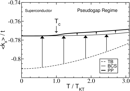
Figure 24: Kinetic energy per bond, $\langle k_{x}\rangle$, as a function of temperature for non interacting tight-binding electrons (TB), the BCS solution (BCS), and the phase fluctuation (PP) model for $\mu=0$ $(\langle n\rangle=1)$. The large vertical arrows indicate the increase in KE upon pairing, relative to the free tight-binding model, and the small arrows indicate the additional increase due to phase fluctuations. This additional phase fluctuation energy rapidly vanishes near $T_{c}=T_{KT}$, which causes the significant change in the OS upon entering the superconducting state at $T_{KT}=0.1\,t$. Note that the thick line follows the actual KE encountered in this model, when going from the pseudogap to the superconducting regime. Adapted from Ref. ref97, .

the superconducting transition temperature $T_{c}$ and the mean field temperature $T_{MF}$ at which the pairs form, is identified with the pseudogap temperature $T^{\ast}$. They take $T_{KT}\simeq T_{MF}/4$ with $T_{KT}=0.1\,t$. In Fig. 24, reproduced from Ref. ref97, , we show the KE per bond, $\langle k_{x}\rangle$ as a function of the reduced temperature $T/T_{KT}$. Here

$$\langle k_{x}\rangle=-t\sum\limits_{\sigma}\left\langle c^{\dagger}_{i\sigma}c_{i+x,\sigma}+c^{\dagger}_{i+x.\sigma}c_{i\sigma}\right\rangle.$$ (38)

The dashed curve is the result of the simple tight-binding Hamiltonian [$K$ of Eq. (34) only] for zero chemical potential and $\langle n\rangle=1$. The light solid line is the result of BCS mean field and the heavy solid line the result obtained by taking into account phase fluctuations within the preformed pair model. The mean field BCS condensation increases the KE above its tight-binding value and the phase fluctuations provide an additional KE increase which vanishes at $T_{c}=T_{KT}$ and this causes significant

Figure 25: Kinetic energy contribution from phase fluctuations $\delta\langle k_{x}\rangle\equiv\langle k_{x}\rangle_{PP}-\langle k_{x}\rangle_{BCS}$. One can clearly see the sharp decrease of KE near the Kosterlitz-Thouless transition $T_{KT}=0.1\,t\equiv T_{c}$. $\Delta E_{k}$ gives an estimate of the kinetic condensation energy. Adapted from Ref. ref97, .

change in the OS as the superconducting state is entered at $T_{KT}=0.1\,t$ in this model calculations. The KE gain from the phase fluctuations $\delta\langle k_{x}\rangle\equiv\langle k_{x}\rangle_{PP}-\langle k_{x}\rangle_{BCS}$ is shown in Fig. 25 which shows a sharp decrease in KE near the Kosterlitz-Thouless transition and $\Delta E_{k}$ gives an estimate of the KE condensation $\propto 0.003\,t$ of the same order as was found in other models. However, this is not the KE change between normal and superconducting state at $T=0$ as discussed previously. Rather it is a change in KE due to the suppression of phase fluctuations present in the pseudogap state. At $T_{c}=T_{KT}$ the phases become locked in and $\delta\langle k_{x}\rangle$ consequently becomes zero. The change in KE on formation of the Cooper pairs is never explicitly considered in this model as the pairs are assumed to form at a much higher temperature $T=T^{\ast}=0.4\,t$.

V.2 The $D$-density Waves, Competing Order Model

There are other very different models that have been proposed for the pseudogap state which exists at temperatures above the superconducting state in the underdoped regime. One proposal is $D$-density wavesref98 ; ref99 ; ref100 ; ref101 ; ref102 ; ref103 ; ref103a ; ref104 ; ref105 ; ref106 (DDW) which falls into the general category of competing interactions. The view is that a new phase, not superconducting, but having a gap with $d$-wave symmetry, forms at $T^{\ast}$ and the superconductivity which arises only at some lower temperature $T_{c}$ is based on this new ground state.ref98 ; ref99 ; ref100 ; ref101 ; ref102 ; ref103 ; ref103a ; ref104 ; ref105 ; ref106 ; ref107 ; ref108 ; ref109 ; ref110 ; ref111 ; ref112 ; ref113 ; ref114 The DDW state breaks time reversal symmetry because it introduces bond currentsref115 ; ref116 with associated small magnetic moments and a gap forms at the antiferromagnetic Brillouin zone boundary. The mean field DDW Hamiltonian is

$$H=\sum\limits_{{\bf k},\sigma}\left[\left(\epsilon_{\bf k}-\mu\right)c^{\dagger}_{{\bf k}\sigma}c_{{\bf k}\sigma}+iD_{\bf k}c^{\dagger}_{{\bf k}\sigma}c_{{\bf k}+{\bf Q}\sigma}\right],$$ (39)

where the sum on k ranges over the entire Brillouin zone and Q is the commensurate wave vector $(\pi/a,\pi/a)$. Here $D_{\bf k}=D_{0}\left[\cos(k_{x}a)-\cos(k_{y}a)\right]/2$ with $D_{0}$ the gap amplitude. Within a mean field approximation the probability of occupation of the state $|{\bf k}\sigma\rangle$ is given byref112

$$n_{{\bf k}\sigma}(T) = \frac{1}{2E_{\bf k}}\left\{E_{\bf k}\left[f(T,\xi_{+{\bf k}})+f(T,\xi_{-{\bf k}})\right]\right.$$ (40)

$$\left.+\epsilon_{\bf k}\left[f(T,\xi_{+{\bf k}})-f(T,\xi_{-{\bf k}})\right]\right\},$$

where $\xi_{\pm{\bf k}}=-\mu\pm E_{\bf k}$ and $E_{\bf k}=\sqrt{\epsilon_{\bf k}^{2}+D_{\bf k}^{2}}$. The number density is

$$n(T)=\frac{2}{N}\sum\limits_{{\bf k}\in{\rm MBZ}}\left[f(T,\xi_{-{\bf k}})+f(T,\xi_{+{\bf k}})\right],$$ (41)

where the sum over k is restricted to half the original Brillouin zone, i.e.: to the magnetic Brillouin zone (MBZ). The KE from Refs. ref108, , ref113, , and ref114, is denoted by $W(D,T)$ and is

$$W(D,T)=\frac{2}{N}\sum\limits_{{\bf k}\in{\rm MBZ}}\frac{\epsilon_{\bf k}^{2}}{E_{\bf k}}\left[f(T,\xi_{+{\bf k}})-f(T,\xi_{-{\bf k}})\right].$$ (42)

Here and later in this section we give formulas only for the simpler case of $t^{\prime}=0$, i.e.: only nearest neighbors. The results to be presented, however, are based on straightforward generalizations that include second nearest neighbors hopping.

Aristov and Zeyherref119 calculated the optical conductivity in the DDW model with and without vertex corrections to the usual current operator. The previous work of Valenzuela et al.ref110 was without vertex corrections as is the more recent work of Gerami and Nayakref120 who, however, consider the effect of anisotropic scattering. These authors use a current operator which includes a term proportional to the gap velocity $\nabla_{\bf k}D_{\bf k}$ which is

Figure 26: Restricted optical sums with (solid line) and without (dot-dashed line) vertex corrections, and Drude weights with (dashed line) and without (dotted line) vertex corrections. Adapted from Ref. ref119, .

introduced so as to ensure charge conservation as is discussed in more detail by Benfatto et al.ref113 Here we follow Aristov and Zeyherref119 and show in Fig. 26 their results for the optical spectral weight as a function of temperature $T$ in units of the hopping parameter $t$. The solid curve is with and the dash-dotted curve is without vertex corrections. We see that while vertex corrections have changed the magnitude of the OS they have changed much less its temperature dependence which is somewhat more pronounced in the solid curve. In both cases the OS decreases with decreasing temperature as was the case in BCS theory. Also shown in Fig. 26 are results for the Drude weight separately, dashed and dotted lines with and without vertex corrections. We see that it is also strongly enhanced by vertex corrections. In Fig. 27 we reproduce results of Aristov and Zeyherref119 for the conductivity $\sigma(\omega)$ vs frequency $\omega$ for $t=0.25\,$eV, $t^{\prime}=0.076$, $T=0.001$, $n=0.4$ and a scattering rate of $1/\tau=0.01$. It is seen that both the Drude region (intra-band) and the inter-band transitions which set in at higher $\omega\geq 0.2$ are larger when vertex corrections are included but that beyond $\omega\geq 0.3$ the two curves merge and the vertex corrections are no longer important.

In the continuum limit of the DDW model Valenzuela et al.ref110 have obtained useful analytic results for intra (Drude) and inter (verticle transitions) separately. Vertex

Figure 27: Optical conductivity $\sigma(\omega)$ with (solid line) and without (dashed line) vertex corrections. Adapted from Ref. ref119, .

corrections are neglected and the limit of zero impurity scattering was taken. They find

$$\sigma_{intra}(T,\omega)=-\delta(\omega)\pi e^{2}\int\limits_{-\infty}^{\infty}\!d\nu\,\left[\frac{\partial f(t,\nu)}{\partial\nu}\right]g_{1}(\nu),$$ (43)

with

$$g_{1}(\nu)=(\hbar v_{F})^{2}N(0)\frac{2}{\pi}\int\limits_{0}^{\pi/2}\!d\theta\,\Re{\rm e}\sqrt{1-\frac{D_{0}^{2}}{(\mu+\nu)^{2}}\cos^{2}\theta},$$ (44)

which can be written in terms of elliptic integrals. Here, $v_{F}$ is the Fermi velocity. Note also that the Fermi factor $f(T,\nu)$ has $\mu=0$ and the chemical potential has been transfered to $g_{1}(\nu)$. For the inter-band

$$\sigma_{inter}(T,\omega)=(\hbar v_{F})^{2}N(0)\frac{1}{\pi}\left(\frac{2D_{0}}{\omega}\right)^{2}\int_{0}^{\pi/2}\!d\theta\,\Re{\rm e}\left[\frac{\cos^{2}\theta}{\sqrt{1-\left(\frac{2\Delta}{\omega}\right)^{2}\cos^{2}\theta}}\right]B(T,\omega),$$ (45)

where $B(T,\omega)$ is a universal thermal factor

$$B(T,\omega)=\frac{\pi e^{2}}{\omega}\frac{\sinh(\beta\omega/2)}{\cosh(\beta\mu)+\cosh(\beta\omega/2)},\qquad\beta=\frac{1}{k_{B}T},$$ (46)

which at $T=0$ becomes proportional to a theta function $\theta(\omega-2|\mu|)$. This provides a low energy cutoff to the inter-band transitions. When impurity scattering is included the delta function $\delta(\omega)$ in Eq. (43) broadens into a Lorentzian and temperature leads to the overlap of the two contributions as seen in Fig. 27.

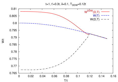
Figure 28: (Color online) Optical spectral weight in the presence of a $t^{\prime}$ term in the band dispersion. Here $W(D,T)$ (Eq. (42), dash-dotted line), $W^{DDW}(D,T)$ (Eq. (47) (solid line) are shown together with $W(T)$ (dashed line) which is for the non interacting case. The parameters are $t^{\prime}=0.3\,t$, $T_{DDW}=0.12\,t$, $D(0)=4T_{DDW}$, and the doping $\delta=0.1$. The chemical potential is evaluated self consistently at each temperature. Observe that near $T_{DDW}$ a small decrease of $W^{DDW}$ with respect to $W(T)$ is seen, due to the change of chemical potential near $T_{DDW}$. Adapted from Ref. ref113, .

We note that the kinetic energy shows the same trend in its temperature dependence as does the OS of Fig. 26. This is shown in Fig. 28 which we took from the work of Benfatto et al.ref113 and where it is denoted by $W(D,T)$ as the dash-dotted curve for the parameters shown in the figure and described in the caption. We see the same decreasing trend with decreasing temperatures as for the OS. There are two other curves, the dashed one is for a pure tight-binding band with no DDW and is included for comparison. The solid curve is for $W^{DDW}(D,T)$ given by

$$W^{DDW}(D,T)=-\frac{1}{N}\sum\limits_{\bf k}^{MBZ}E_{\bf k}\left[f(T,\xi_{+{\bf k}})-f(T,\xi_{-{\bf k}})\right]$$ (47)

(again in units of $\pi e^{2}/\hbar^{2}$) in the notation of Benfatto et al.ref113 ; ref114 and requires explanation. It was obtained from a current operator which was modified to ensure charge conservation without the need for vertex corrections. This current operator has been used in other worksref108 ; ref120 as well. As noted by Aristov and Zeyherref119 , however, such a procedure tends to overestimate the conductivity at higher frequencies and the OS now shows an increase as $T$ is decreased.

We can also add a mean field BCS term

$$H^{\prime}=\sum\limits_{\bf k}\left[\Delta^{\ast}_{\bf k}c_{-{\bf k}\downarrow}c_{{\bf k}\uparrow}+h.c.\right],$$ (48)

to the Hamiltonian (39), where $\Delta_{\bf k}$ is the superconducting order parameter. $\Delta_{\bf k}=\Delta_{0}\left[\cos(k_{x}a)-\cos(k_{y}a)\right]$ with $\Delta_{0}$ the superconducting gap amplitude. In this case the OS in units of $\pi e^{2}/\hbar^{2}$ is given by

$$W^{DDW}(D,\Delta,T) = \frac{2}{N}\sum\limits_{\bf k}^{\rm MBZ}E_{\bf k}\left[\frac{\xi_{+{\bf k}}}{E_{+{\bf k}}}\tanh\left(\frac{E_{+{\bf k}}}{2T}\right)\right.$$ (49)

$$\left.-\frac{\xi_{-{\bf k}}}{E_{-{\bf k}}}\tanh\left(\frac{E_{-{\bf k}}}{2T}\right)\right],$$

with $E_{\pm{\bf k}}=\sqrt{\xi^{2}_{\pm{\bf k}}+\Delta^{2}_{\bf k}}$.

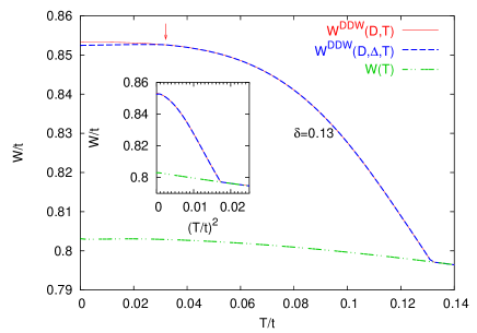
Figure 29: (Color online) Optical spectral weight in units of $e^{2}\pi/\hbar^{2}$ in the normal state (dash double-dotted line), in the DDW state Eq. (47) (solid line) and in DDW+SC state Eq. (49) (dashed line). The values of parameters are for the doping $\delta=0.13$ [$D_{0}(T=0)=0.92\,t$, $\Delta(T=0)=0.064\,t$, see Refs. ref107, and ref108, for further details. The critical temperature is marked by the arrow. Observe that the decrease of $W^{DDW}(D,\Delta,T)$ below $T_{c}$ is small. Inset: spectral weight plotted as a function of $(T/t)^{2}$. Adapted from Ref. ref114, (see also Ref. ref108, ).

In Fig. 29 we show results reproduced from Benfatto and Sharapovref114 for the effect of combined DDW and superconducting transition described by Eq. (49). The optical weight is given in units of $t$ (nearest neighbor hopping) as is the temperature. The dash-double-dotted curve $[W(T)]$ is for reference and gives results for the tight binding band without interactions while the solid lines gives $W^{DDW}(D,T)$ as before and the dashed curve is for $W^{DDW}(D,\Delta,T)$ which includes the effect of a $d$-wave superconducting gap of amplitude $\Delta$. We note that, as expected, this leads to an increase in KE with respect to the pure DDW case and, therefore, a drop in the OS.

It is clear that, as yet, a complete theory of the OS in the DDW model does not exist. The calculations of Aristov and Zeyherref119 with vertex corrections properly accounted for give the opposite temperature dependence than found experimentally. This theory, however, does not include correlations beyond those directly responsible for the DDW transition. It is clear from what we have described here that correlations leading to lifetime effects need to be included as these are very closely related to the observed temperature dependence of the OS and cannot be ignored.

VI Optical Spectral Weight Distribution

In this review we focused mainly on the OS for a single band

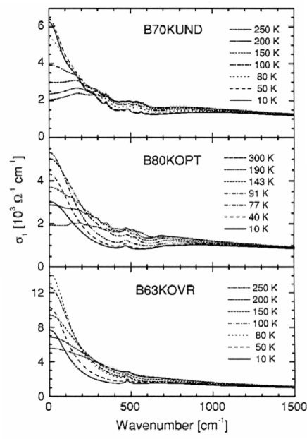
Figure 30: Selection of conductivity spectra for three BSCCO samples, underdoped, $T_{c}=70\,$K (B70KUND, top frame), optimally doped, $T_{c}=80\,$K (B80KOPT, middle frame), and overdoped, $T_{c}=63\,$K (B63KOVR, bottom frame). For the B70KUND sample, within the showed spectral range, the spectra at $50\,$K and $10\,$K are indistinguishable. Adapted from Ref. ref47, .

integrated over all energies of relevance. As is seen from Eq. (1) this quantity can be computed from a knowledge of the single electron spectral density $A({\bf k},\omega)$ which determines the probability of occupation $n_{{\bf k},\sigma}$ of the state $|{\bf k},\sigma\rangle$. This is a much simpler problem than computing the frequency dependent conductivity from a Kubo formula which involves the two-particle Green’s functions. However, calculating the full frequency dependent conductivity cannot be avoided if one wishes to discuss the optical spectral weight distribution. The partial integration of $\sigma_{1}(T,\omega)$ to a maximum $\omega$ equal to $\omega_{M}$ has proved be very useful and has provided valuable information about normal and superconducting state beyond what is obtained from the OS itself. We give here only two examples. In Fig. 30 we reproduce the conductivity data of Santander-Syro et al.ref47 in three BSCCO samples, underdoped $T_{c}=70\,$K (B70KUND), optimally doped at $T_{c}=80\,$K (B80KOPT), and overdoped at $T_{c}=63\,$K (B63KOVR) at the various temperatures noted in the figure. From these data it is possible to calculate $W(T,\omega_{M})=\int_{0^{+}}^{\omega_{M}}d\omega\,\sigma_{1}(T,\omega)$ at various temperatures. Here the $0^{+}$ indicates that

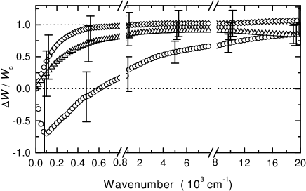
Figure 31: Rato $\Delta W/W_{S}$ vs frequency showing the exhaustion of the Ferrell-Glover-Tinkham sum rule at conventional energies for the OVR (diamonds) and OPT (triangles) samples. An unconventional ($\sim 16000\,$cm^-1 or $2\,$eV) energy scale is required for the UND sample (circles). Note that the frequency scale changes at 800 and $8000\,$cm^-1. The changes in spectral weight are taken between $80\,$K - $10\,$K, $91\,$K - $10\,$K, and $100\,$K - $10\,$K for the OVR, OPT, and UND samples, respectively. Adapted from Ref. ref47, .

the delta function representing the condensate has been left out. In Fig. 31 we reproduce the experimental results of Santander-Syro et al.ref47 for the normalized change in spectral weight $\Delta W/W_{S}$ vs $\omega_{M}$ in $10^{3}\,$cm^-1 based on the data of Fig. 30. Open diamonds, triangles, and circles are for B63KOVR, B80KOPT, and B70KUND, respectively. Note the two breaks in the horizontal scale for $\omega_{M}$ at 800 and $8000\,$cm^-1. The change in optical spectral weight is slightly different

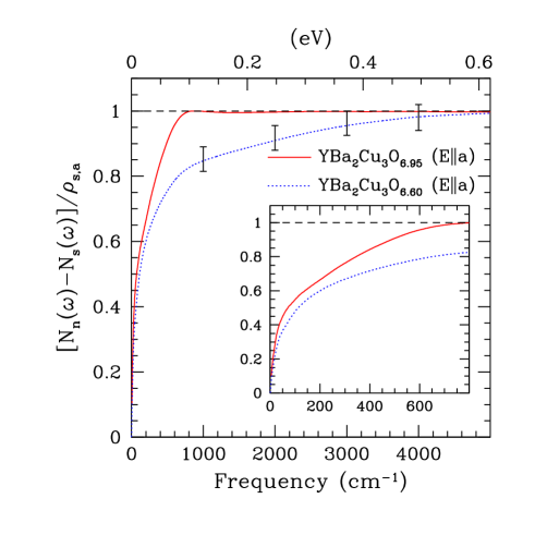
Figure 32: (Color online) The normalized weight of the condensate [$N_{n}(\omega)-N_{s}(\omega)]/\rho_{s,a}$ vs $\omega$ for optimally doped YBCO_6.95 (solid line) and underdoped YBCO_6.60 (dotted line) along the $a$-axis direction. The condensate for the optimally doped material has saturated by $\simeq 800\,$cm^-1, while in the underdoped material the condensate is roughly 80% formed by this frequency, but the other 20% is not recovered until much higher frequencies. The error bars on the curve for the underdoped material indicate the uncertainty associated with the Ferrell-Glover-Tinkham sum rule. Inset: The low-frequency region. Adapted from Ref. ref121, .

for the OVR, OPT, and UND samples as indicated in the caption. Note the approach to its asymptotic value of one. For the overdoped case the scale is $\sim 600\,$cm^-1 while for the UND sample it is much larger and of order $2\,$eV. These experiments clearly reveal a fundamental difference in behavior between overdoped and underdoped samples. This was also observed in the YBCO series. Data from Homes et al.ref121 are reproduced in Fig. 32 for electric field E parallel to the $a$-axis in YBCO_6.95 (solid line) and YBCO_6.60 (dotted line). For the optimally doped sample the OS is rapidly saturated ($\omega_{M}\simeq 800\,$cm^-1) while for the underdoped case a frequency of about $9000\,$cm^-1 is needed.

For a BCS $s$-wave superconductor the expectation is that the saturation of the OS should occur at a frequency $\omega$ a few times the gap $\Delta$ even if the system is dirty with scattering rates $\stackrel{{\scriptstyle>}}{{\sim}}2\Delta$, Refs. ref121, and ref122, . However, superconductors are better described by Eliashberg theory which properly accounts for coupling of the electrons to phonons. In this case the weight in the coherent quasiparticle part of the spectral function is $Z=1/(1+\lambda)$ where $\lambda$ is the mass enhancement factor. The rest of the spectral weight lies in an incoherent phonon induced band at higher energy, usually in the infrared. This part of the spectral function $A({\bf k},\omega)$ contributes the so called Holstein band to the optical conductivity. Only the quasiparticle part is included in BCS theory, yet for $\lambda>1$, say, more of the electron spectral weight is in the incoherent part than one finds in the coherent part. This part introduces a new energy scale into the problem, namely, an average phonon energy and it is no longer true to say that readjustment of optical spectral weight on entering the superconducting state can only occur on the scale of twice the gap. In fact, one should expect that when the electrons pair, an absorption process involving a phonon $\omega_{E}$ would be changed and shifted to an energy of $2\Delta+\omega_{E}$, thus shifting the Holstein band to higher energies and, hence, the incoherent part of the optical spectral weight in the superconducting state extends to higher energies. This implies that

Figure 33: Top frame: Optical spectral weight $W(\omega,T)=\int_{0^{+}}^{\omega}\!d\nu\,\sigma_{1}(\nu)$ for various cases as a function of $\omega$. The dotted (dash-double-dotted) curve is for the normal state at $T=10\,$K ($T=95\,$K), the solid curve for the superconducting state at $T=10\,$K. The dashed (dash-dotted) curve is the difference curve between superconducting at $T=10\,$K and normal states at $T=10\,$K ($T=95\,$K). The approach of the difference curve to its saturated large $\omega$ value depends significantly on the temperature used for the subtracted normal state. The thin dash-double-dotted horizontal line is the value of the condensate contribution (penetration depth). The bottom frame shows the real part of the conductivity for the normal state at $T=293\,$K (dashed curve), $T=95\,$K (dash-dotted curve), $T=10\,$K (dotted curve), and for the superconducting state at a $T=10\,$K (solid curve). All curves are for YBCO_6.95 with the impurity parameter given in Ref. ref122a, .

$\int_{0^{+}}^{\omega}\!d\nu\,[\sigma_{N}(T,\nu)-\sigma_{S}(T,\nu)]$ for large $\omega$ should saturate from above rather than from below as is the case in BCS. This is known from the $s$-wave phonon mediated caseref129 and is illustrated in Fig. 33 taken from Carbotte and Schachingerref122a for a $d$-wave superconductor using for $I^{2}\chi(\omega)$ an MMP form. What is shown in the top frame are numerical results for $W(T,\omega)$ defined as $W(T,\omega)=\int_{0^{+}}^{\omega}\!d\nu\,\sigma_{1}(T,\nu)$. The real part of the conductivity $\sigma_{1}(T,\omega)$ in arbitrary units on which these various curves are based are shown in the bottom frame. These calculations are all done for infinite bands and corresponding Eliashberg equations for a $d$-wave superconductor so that the Ferrell-Glover-Tinkham sum rule holds, i.e.: the total optical spectral weight is conserved between normal and superconducting state.ref123 ; ref124 Parameters were varied to get a good fit to data on YBCO_6.95. The reader is referred to the paper of Schachinger and Carbotteref33 for details. Some impurity scattering in the unitary limit is included to get Fig. 33. $W(T,\omega)$ is shown for $\omega$ up to $250\,$meV. The solid curve is in the superconducting state at $T=10\,$K and the dotted the normal state at the same temperature. $W_{N}(T)$ (normal state) rises much more rapidly at small $\omega$ than does $W_{S}(T)$ (supercond. state) and goes to much larger values. The difference $W_{N}(T=10\,{\rm K},\omega)-W_{S}(T=10\,{\rm K},\omega)$ (dashed curve) is the amount of optical spectral weight that has been transferred to the condensate between $(0^{+},\omega)$. This curve rapidly grows to a value slightly below the horizontal line representing the condensate contribution to the total sum rule. After this the remaining variation is small with a shallow minimum around $30\,$meV followed by a broad peak around $60\,$meV which falls above the thin dash-double-dotted horizontal line before gradually falling again towards its asymptotic value which must be equal to the condensate contribution. All these features can be understood from a consideration of the curves for $\sigma_{1}(T,\omega)$ given in the bottom frame. Comparing dotted and solid curves, we see that they cross at three places on the frequency axis at $\omega_{1}\approx 8\,$meV, $\omega_{2}\approx 32\,$meV, and $\omega_{3}\approx 130\,$meV. These features are a result of the shift in incoherent background towards higher energies due to the opening of the superconducting gap.

In an actual experiment it is usually not possible to access the normal state at $T=10\,$K (say) so that $W_{N}(T=95\,{\rm K},\omega)$ just above $T_{c}=92\,$K needs to be used (dash-double dotted curve). The difference $W_{N}(T=95\,{\rm K},\omega)-W_{S}(T=10\,{\rm K},\omega)$ is shown as the dash-dotted curve in the top frame and is seen to merge with the dashed curve only at higher values of $\omega$. Reference to the bottom frame shows that the real part of the normal state conductivity at $T=95\,$K (dash-dotted curve) is much broader than at $T=10\,$K (dotted curve) and this accounts for the slower rise towards saturation of the dash-dotted as compared to the dashed curve in the top frame. We note, however, that $W_{N}(T=95\,{\rm K},\omega)-W_{S}(T=10\,{\rm K},\omega)$ still approaches the penetration depth curve from above but much of the structure seen in the dashed curve is lost by using the data for the normal state at $T=95\,$K rather than at $T=10\,$K. Nevertheless, the energy scale over which the condensate is formed is set by the energy of the spin fluctuation spectra which extends up to $400\,$meV in our calculations and not by the gap value $2\Delta_{0}$.

VII Summary

The temperature dependence of the OS has recently been measured up to $\sim 300\,$K in the normal state of several cuprates as well as in the superconducting state. Some controversy remains about details such as the exact temperature dependence followed in the normal state. However, it seems established that underdoped samples show anomalous behavior when they enter the superconducting state. For a normal BCS superconductor the KE should increase while it is seen to decrease over its extrapolated normal state value. This, on its own, does not mean that the condensation is purely driven by the kinetic energy but it does mean that we are faced with non BCS behavior. For optimally doped samples the change in KE is close to zero with a definite crossover to conventional behavior in overdoped samples. For the normal state many experiments, but not all, give a $T^{2}$ dependence of the OS. Recent DMFT calculations for the Hubbard model provide evidence for a universal $T^{2}$ behavior in the normal state. We argue, however, that such a law is not robust when electron-boson theories for the interaction are considered. In this case, if the boson energy is low, a linear in $T$ dependence can result and by implication other dependences on $T$ can arise for different electron-boson spectral densities. The same holds for coupling to spin fluctuations in the NAFFL model. The issue of the temperature dependence of the underlying normal state OS or KE impacts the analysis of the change in KE that results from the superconducting condensation. If the normal state KE decreases faster at low temperatures than it does above $T_{c}$ (as we have seen in some models) this could be interpreted as an anomalous superconducting state, yet it would not be. On the other hand, in the NAFFL model as well as in electronic models more generally, anomalous behavior of the optical sum can be understood as due to the so called collapse of the inelastic scattering rates in the superconducting state if this reduces the effect of spin fluctuations at small $\omega$. Such a hardening of the spin fluctuation spectrum is thought to be a viable explanation for the peak in the microwave conductivity which is observed at a temperature considerably below $T_{c}$. This effect, which can be modeled by a low energy cutoff in the electron-spin fluctuation spectral density, results directly in a decrease in KE of the underlying normal state as additional coherence sets in with the establishment of superconductivity. This idea is related to the work of Norman and Pépinref78 ; ref79 who model directly the charge carrier self energy rather than go through the electron-boson spectral function. They take the imaginary part of the self energy $(\Sigma_{2})$ to be large in the normal state (incoherence) and increase coherence in the superconducting state through a low frequency cutoff below which $\Sigma_{2}$ is zero. Another related model, which is even simpler, is to use a temperature dependent elastic scattering time which collapses in the superconducting state as $\alpha T^{4}$ with $\alpha$ taken from microwave experiments. All these mechanisms can easily provide savings in KE sufficiently large to explain the OS experiments. None, however, are fully quantitative at present. They also need to be extended to the overdoped side of the phase diagram. In this case one would expect the corresponding microwave peak to be greatly reduced and be more conventional. More sophisticated, but perhaps less transparent numerical calculations based on the Hubbard model and on the $t$-$J$ model have also found that, as a function of doping, the KE can favor pairing in underdoped systems while for the overdoped case it behaves as for a conventional superconductor. Earlier calculations based on the Hubbard model, however, give kinetic energy pairing even on the overdoped side of the phase diagram. By contrast, calculations based on the negative $U$ Hubbard model used to describe the BCS-BE crossover do capture the observed change in sign of the kinetic energy difference.

In Ref. ref122, and, more recently, in Ref. ref53, the possibility is raised that some of the effects studied in this review may arise from infinite bands when a finite cutoff is applied to the optical sum integral as it must in the analysis of experimental data. Certainly, for the high $T_{c}$ oxides there is no clear ‘ending’ of one band at a given energy followed by a gap before the next band sets in at higher energies. Instead, only a minimum is observed in the real part of the conductivity as a function of $\omega$ at about $1.2\,$eV. This energy has been taken as the cutoff on the transitions associated with the single band of interest. This cutoff is also roughly consistent with what is known about the width in energy of the bands in the oxides. Nevertheless, ambiguity remains and a theoretical study of overlapping bands and what this might imply for the single band sum rule would be valuable in clarifying this situation further.

Much remains to be done to connect weak coupling approaches with the more numerical strong coupling results. There is also a need to get more accurate data which could resolve the experimental debate that still goes on and to achieve quantitative agreement with experiments. What is clear, however, is that such experiments can give useful information on the correlation effects that are involved and they certainly have shown that superconductivity on the underdoped side of the phase diagram of the cuprates is likely to be unconventional. It cannot be understood on the basis of a simple BCS model or an Eliashberg model with conventional phonons as these are not expected to change much as superconductivity sets in and they are distributed over a large energy range rather than peaked at low $\omega$. However, we stress again that as we have seen in one case, a small upturn in the OS at low temperature in the superconducting state can arise in spin fluctuation models without a readjustment of the electron-spin fluctuation spectrum, when the spin fluctuation energy in the MMP spin susceptibility is sufficiently small. While this upturn is less in the superconducting state than in its normal state at this same temperature (below $T_{c}$) it is above the value extrapolated to $T=0$ from the normal state above $T_{c}$. A second important conclusion of this review is that lifetime effects are important in determining the temperature dependence of the OS in both normal and superconducting state. These have to be accounted for in any definitive theory of this effect.

There is a need to continue to explore other models such as phase fluctuations. In particular, the $D$-density wave model as a possible competing order for the pseudogap phase has not yet included effects of correlations beyond those that lead to the DDW order, i.e: lifetime effects which we have argued to be central to this problem. More work involving other models of interaction effects so as to understand what other temperature laws are possible for the OS vs $T$ would also be useful.

- (1) C. Campuzano, M.R. Norman, and M. Randeria, in: The Physics of Superconductivity; Conventional and High-Tc Superconductors, edited by K.-H. Bennemann and J. B. Ketterson (Springer, Berlin, 2003), Vol. II, p. 167.
- (2) A. Damascelli, Z. Hussain, and Z.X. Shen, Rev. Mod. Phys. 75, 473 (2003).
- (3) H. Matsui, K. Terashima, T. Sato, T. Takahashi, M. Fujita, and K. Yamada, Phys. Rev. Lett. 95, 017003 (2005).
- (4) D.A. Bonn and W.N. Hardy, in: Physical Properties of High Temperature Superconductors, edited by D.M. Ginsberg (World Scientific, Singapore, 1996), Vol. 5, p. 7.
- (5) C.C. Tsuei and J.R. Kirtley, in: The Physics of Superconductivity; Conventional and High-Tc Superconductors, edited by K.-H. Bennemann and J. B. Ketterson (Springer, Berlin, 2003), Vol. I, p. 648.
- (6) M.C. Nuss, P.M. Mankiewich, M.L. O’Malley, E.H. Westerwick, and P.B. Littlewood, Phys. Rev. Lett. 66, 3305 (1991).
- (7) D.A. Bonn, P. Dosanjh, R. Liang, and W.N. Hardy, Phys. Rev. Lett. 68, 2390 (1992).
- (8) D.B. Romero, C.D. Porter, D.B. Tanner, L. Forro, D. Mandrus, L. Mihaly, G.L. Carr, and G.P. Williams, Phys. Rev. Lett. 68, 1590 (1992).
- (9) E.J. Nicol and J.P. Carbotte, Phys. Rev. B 44, 7741 (1991).
- (10) Shih-Fu Lee, D.C. Morgan, R.J. Ormeno, D.M. Broun, R.A. Doyle, J.R. Waldram, and K. Kadowaki, Phys. Rev. Lett. 77, 735 (1996).
- (11) S.M. Broun, D.C. Morgan, R.J. Ormeno, S.F. Lee, A.W. Tyler, A.P. Mackenzie, and J.R. Waldram, Phys. Rev. B 56, R11443 (1997).
- (12) J.E. Hirsch, Phys. Lett. A 134, 451 (1989).
- (13) J.E. Hirsch, Physica C 199, 305 (1992); Physica C 201, 347 (1992).
- (14) J.E. Hirsch and F. Marsiglio, Phys. Rev. B 39, 11515 (1989).
- (15) J.E. Hirsch and F. Marsiglio Physics C 331, 150 (2000); Phys. Rev. B 62, 15131 (2000).
- (16) P.W. Anderson, Science 279, 1196 (1998); in: The Theory of Superconductivity in the High Cuprates (Princeton University Press, Princeton, 1997).
- (17) S. Chakravarty, Eur. Phys. J. B 5, 337 (1998).
- (18) R. Kubo, J. Phys. Soc. Japan 12, 570 (1957).
- (19) D.N. Basov, S.I. Woods, A.S. Katz, E.J. Singley, R.C. Dynes, M. Xu, D.G. Hinks, C.C. Homes, and M. Strongin, Science 283 49 (1999).
- (20) L.B. Ioffe and A.J. Millis, Science 285, 1241 (1999); Phys. Rev. B 61, 9077 (2000).
- (21) Wonkee Kim and J.P. Carbotte, Phys. Rev B 61, 11886R (2000); 62, 8661 (2000); 63, 140505R (2001); 63, 054526 (2001); 64, 104501 (2001).
- (22) N. Kumar and A.M. Jayannavar, Phys. Rev. B 45, 5001 (1992).
- (23) P.W. Anderson and Z. Zou, Phys. Rev. Lett. 60, 132 (1988); 60, 2557 (1988).
- (24) A.J. Leggett, Braz. J. Phys. 22, 129 (1992); M. Turlabov and A.J. Leggett, Phys. Rev. B 62, 064518 (2001).
- (25) Z. Tesanovic, Phys. Rev. B 36, 2364 (1987); 38, 2489 (1988).
- (26) J. Halbritter, J. Supercond. 11, 231 (1998).
- (27) W.A. Atkinson and J.P. Carbotte, Phys. Rev. B 52, 10 601 (1995); 55, 3230 (1997); 55, 12 748 (1997).
- (28) W.C. Wu, W.A. Atkinson, and J.P. Carbotte, J. Supercond. 11, 305 (1997).
- (29) T. Xiang and J.M. Wheatley, Phys. Rev. Lett. 77, 4632 (1996).
- (30) P.J. Hirschfeld, S.M. Quinlan, and D.J. Scalapino, Phys. Rev. B 55, 12 742 (1997).
- (31) E.H. Kim, Phys. Rev. B 58, 2452 (1997).
- (32) M.J. Graf, M. Palumbo, D. Rainer, and J.A. Sauls, Phys. Rev. B 52, 10 588 (1995).
- (33) E. Schachinger and J.P. Carbotte, Phys. Rev. B 64, 094501 (2001).
- (34) D. van der Marel, H.J.A. Molegraaf, C. Presura, and L. Santoso, in Concepts in Electron Correlations, edited by A. Hewson and V. Zlatic (Kluwer, 2003) p. 7.
- (35) G. Deutscher, A.F. Santander-Syro, and N. Bontemps, Phys. Rev. B 72, 092504 (2005).
- (36) F. Carbone, A.B. Kuzmenko, H.J.A. Molegraaf, E. van Heumen, V. Lukovac, F. Marsiglio, D. van der Marel, K. Haule, G. Kotliar, H. Berger, S. Courjault, P.H. Kes, M. Li, cond-mat/0605209 (unpublished).
- (37) R.A. Ferrell and R.E. Glover, Phys. Rev. 109, 1398 (1958).
- (38) M. Tinkham and R.B. Ferrell, Phys. Rev. Lett. 2, 331 (1959).
- (39) F. Marsiglio, F. Carbone, A. Kuzmenk, and D. van der Marel, cond-mat/0606688 (unpublished).
- (40) A. Knigavko, J.P. Carbotte, and F. Marsiglio, Phys. Rev. B. 70, 224501 (2004).
- (41) F. Marsiglio and J.E. Hirsch, Phys. Rev. B 41, 6435 (1990); Physica C 165, 71 (1990).
- (42) M.A. Quijada, D.B. Tanner, R.J. Kelley, M. Onellion, H. Berger, and G. Margaritondo, Phys. Rev. B 60, 14917 (1999).
- (43) L. Benfatto, F. Marsiglio, and J.P. Carbotte, cond-mat/0603661 (unpublished).
- (44) A.E. Karakozov and E.G. Maksimov, cond-mat/0511185 (unpublished).
- (45) P. Monthoux and D. Pines, Phys. Rev. B 47, 6069 (1993); 49, 4261 (1994).
- (46) P. Monthoux, A.V. Balatsky, and D. Pines, Phys. Rev. Lett. 67, 3448 (1991); Phys. Rev. B 46, 14 803 (1992).
- (47) A.J. Millis, H. Monien, and D. Pines, Phys. Rev. B 42, 167 (1990).
- (48) D. Branch and J.P. Carbotte, Can. J. Phys. 77, 531 (1999); J. Superconductivity 12, 667 (1999); 13, 535 (2000).
- (49) A. Abanov, A.V.Chubukov, and J. Schmalian, Adv. in Physics 52, 119 (2003).
- (50) E. Schachinger and J.P. Carbotte, Phys. Rev. B 72, 014535 (2005).
- (51) V. Chubukov, D. Pines, and J. Schmalian, in: The Physics of Superconductivity; Conventional and High-Tc Superconductors, edited by K.-H. Bennemann and J. B. Ketterson (Springer, Berlin, 2003), Vol. I, p. 495.
- (52) A. Toschi, M. Capone, M. Ortolani, P. Calvani, S. Lupi, C. Castellani, Phys. Rev. Lett. 95, 097002 (2005).
- (53) A. Georges, G. Kotliar, M.J. Rozenberg, and W. Krauth, Rev. Mod. Phys. 68, 13 (1996).
- (54) M. Ortolani, P. Calvani, and S. Lupi, Phys. Rev. Lett. 94, 067002 (2005).
- (55) A. Lucarelli, S. Lupi, M. Ortolani, P. Calvani, P. Maselli, M. Capizzi, P. Giura, H. Eisaki, N. Kikugawa, T. Fujita, M. Fujita, and K. Yamada, Phys. Rev. Lett. 90, 037002 (2003).
- (56) A.F. Santander-Syro, R.P.S.M. Lobo, N. Bontemps, Z. Konstantinovic, and H. Raffy, Phys. Rev. Lett. 88, 097005 (2002).
- (57) A.F. Santander-Syro, R.P.S.M. Lobo, N. Bontemps, Z. Konstantinovic, Z.Z. Li, and H. Raffy, Europhys. Lett. 62, 568 (2003).
- (58) A.F. Santander-Syro, R.P.S.M. Lobo, N. Bontemps, W. Lopera, D. Giratá, Z. Konstantinovic, Z.Z. Li, and H. Raffy, Phys. Rev. 70, 134504 (2004).
- (59) H.J.A. Molegraaf, C. Presura, D. van der Marel, P.H. Kes, and M. Li, Science 295, 22 (2002).
- (60) Th.A. Maier, M. Jarrell, A. Macridin, and C. Slezak, Phys. Rev. Lett. 92, 027005 (2004)
- (61) K. Haule and G. Kotliar, cond-mat/0601478 (unpublished).
- (62) G. Grimaldi, E. Cappelutti, and L. Pietrobero, Europhys. Lett. 42, 667 (1998).
- (63) E. Cappelluti, C. Grimaldi, and L. Pietronero, Phys. Rev. B 64, 125104 (2001).
- (64) E. Capeppelluti and L. Pietronero, Phys. Rev. B 68, 224511 (2003).
- (65) F. Doǧan and F. Marsiglio, Phys. Rev. B 68, 165102 (2003).
- (66) A. Knigavko and J.P. Carbotte, Phys. Rev. B 72, 035125 (2005).
- (67) A. Knigavko and J.P. Carbotte, Phys. Rev. B 73, 125114 (2006).
- (68) A. Knigavko, J.P. Carbotte, and F. Marsiglio, Europhys. Lett. 71, 776 (2005).
- (69) F. Marsiglio, M. Schossmann, and J.P. Carbotte, Phys. Rev. B 32, 4965 (1988).
- (70) J.P. Carbotte, E. Schachinger, and J. Hwang, Phys. Rev. B 71, 054506 (2005).
- (71) E. Schachinger and J.P. Carbotte, Phys. Rev. B 62, 9054 (2000).
- (72) J. Hwang, J. Yang, T. Timusk, S.G. Sharapov, J.P. Carbotte, D.A. Bonn, Ruixing Liang, and W.N. Hardy, Phys. Rev. B 73, 014508 (2006).
- (73) A.V. Boris, N.N. Kovaleva, D.V. Dolgov, T. Holden, C.T. Lin, B. Keimer, and C. Bernhard, Science 304, 708 (2004).
- (74) A.B. Kuzmenko, H.J.A. Molegraaf, F. Carbone, and D. van der Marel, Phys. Rev. B 72, 144503 (2005).
- (75) A.F. Santander-Syro and N. Bontemps, Science 304, 708 (2004).
- (76) J.P. Carbotte, E. Schachinger, and D.N. Basov, Nature (London) 401, 354 (1999).
- (77) E. Schachinger, J.P. Carbotte, and D.N. Basov, Europhys. Lett. 54, 380 (2001).
- (78) E. Schachinger and J.P. Carbotte, in: Models and Methods of High-TC Superconductivity: some Frontal Aspects, edited by J.K. Srivastava and S.M. Rao, (Nova Science, Hauppauge, NY, 2003), Vol. II, p. 73.
- (79) P. Bourges, in: The Gap Symmetry and Fluctuations in High Temperature Superconductors, edited by J. Bok, G. Deutscher, D. Pavuna, and S.A. Wolf (Plenum Press, London, 1998), p. 349.
- (80) E. Schachinger and J.P. Carbotte, Phys. Rev. B 65, 064514 (2002).
- (81) A. Hosseini, R. Harris, Saeid Kamal, P. Dosanjh, J. Preston, Ruixing Liang, W.N. Hardy, and D.A. Bonn, Phys. Rev. B 60, 1349 (1999).
- (82) D.A. Bonn, Ruixing Liang, T.M. Risemann, D.J. Baar, D.C. Morgan, K. Zhang, P. Dosanjh, T.L. Duty, A. MacFarlane, G.D. Morris, J.H. Brewer, W.H. Hardy, C. Kallin, and A.J. Berlinsky, Phys. Rev. B 47, 11 314 (1993).
- (83) E. Schachinger and J.P. Carbotte, Phys. Rev. B 57, 13 773 (1998); 57, 7970 (1998).
- (84) E. Schachinger, J.P. Carbotte, and F. Marsiglio, Phys. Rev. B 56, 2738 (1997).
- (85) R.S. Markiewicz, S. Sahrakorpi, M. Lindroos, Hsin Lin, and A. Bansil, cond-mat/0503064 (unpublished) and references therein.
- (86) F. Marsiglio, Phys. Rev. B 73 064507 (2006); Erratum to be published.
- (87) M.R. Norman and C. Pépin, Phys. Rev. B 66, 100506(R) (2002).
- (88) M.R. Norman and C. Pépin, Rep. Progr. Phys. 66, 1547 (2003).
- (89) M.R. Norman and H. Ding, Phys. Rev. B 57, R11089 (1998).
- (90) R. Hlubina and T.M. Rice, Phys. Rev. B 51, 9253 (1995).
- (91) T. Valla, A.V. Fedorov, P.D. Johnson, Q. Li, G.D. Gu, and N. Koshizuka, Phys. Rev. Lett. 85, 828 (2000).
- (92) K.G. Sandeman and A.J. Schofield, Phys. Rev. B 63, 094510 (2001).
- (93) B.P. Stojkovic and D. Pines, Phys. Rev. Lett. 76, 811 (1996).
- (94) C.M. Varma, P.B. Littlewood, S. Schmitt-Rink, A. Abrahams, and A.E. Ruckenstein, Phys. Rev. Lett. 63, 1996 (1989).
- (95) C.M. Varma, Phys. Rev. B 55, 14 554 (1997).
- (96) A.V. Puchkov, D.N. Basov, and T. Timusk, J. Phys.: Condens. Matter 8, 10 049 (1996).
- (97) This was pointed out in footnote 15 of Ref. ref87a, .
- (98) N. Bontemps, R.P.S.M. Lobo, A.F. Santander-Syro, A. Zimmers, cond-mat/0603024 (unpublished).
- (99) J.L. Tallon and J.W. Loram, Physica C 349, 53 (2001).
- (100) A. Toschi, M. Capone, and C. Castellani, Phys. Rev. B 72, 235118 (2005).
- (101) B. Kyung, A. Georges, and A.-M. S. Tremblay, cond-mat/0508645 (unpublished).
- (102) V.J. Emery and S.A. Kivelson, Nature (London) 374, 434 (1995).
- (103) M. Randeria, N. Trivedi, A. Moreo, and R.T. Scalettar, Phys. Rev. Lett. 69, 2001 (1992).
- (104) M. Franz and A.J. Millis, Phys. Rev. B 58, 14 572 (1998).
- (105) N.-J. Kwon and A.T. Dorsey, Phys. Rev. B 59, 6438 (1999).
- (106) I.F. Herbut, Phys. Rev. Lett. 88, 047006 (2002).
- (107) T. Eckl, D.J. Scalapino, E. Arrigoni, and W. Hanke, Phys. Rev. B 66, 140510(R) (2002).
- (108) T. Eckl, W. Hanke, and E. Arrigoni, Phys. Rev. B 68, 014505 (2003).
- (109) T.K. Kopeć, Phys. Rev. B 67, 014520 (2003).
- (110) S. Chakravarty, R.B. Laughlin, D.K. Morr, and C. Nayak, Phys. Rev. B 63, 094503 (2001).
- (111) B. Dòra, A. Virosztek, and K. Maki, Phys. Rev. B 65, 155119 (2002); K. Maki, B. Dòra, M. Kartsovnik, A. Virosztek, B. Korin-Hamzic, and M. Basletic, Phys. Rev. Lett. 90, 256402 (2003).
- (112) S. Chakravarty, H.-Y. Kee, and C. Nayak, Int. J. Mod. Phys. B 15, 2901 (2001).
- (113) J.-X. Zhu, W. Kim, C.S. Ting, and J.P. Carbotte, Phys. Rev. Lett. 87, 197001 (2001).
- (114) X. Yang and C. Nayak, Phys. Rev. B 65, 064523 (2002).
- (115) Q.H. Wang, J.H. Han, and D.H. Lee, Phys. Rev. Lett. 87, 077004 (2001).
- (116) S. Chakravarty, C. Nayak, and S. Tewari, Phys. Rev. B 68, 100504 (2003).
- (117) S. Chakravarty, C. Nayak, S. Tewari, and X. Yang, Phys. Rev. Lett. 89, 277003 (2002).
- (118) S. Tewari, H.-Y. Kee, C. Nayak, S. Chakravarty, Phys. Rev. B 64, 224516 (2001).
- (119) E. Capelutti and R. Zehyer, Phys. Rev. B 59, 6475 (1999).
- (120) L. Benfatto, S. Caprara, and C. DiCastro, Eur. Phys. J. B 17, 95 (2000).
- (121) L. Benfatto, S. Sharapov, and H. Beck, Eur. Phys. J. B 34, 469 (2004).
- (122) D.N. Aristov and R. Zeyher, Phys. Rev. B 70, 212511 (2004).
- (123) B. Valenzuela, E.J. Nicol, and J.P. Carbotte, Phys. Rev. B 71, 134503 (2005).
- (124) Wonkee Kim and J.P. Carbotte, Phys. Rev. B 66, 033104 (2002).
- (125) Wonkee Kim, J.X. Zhu, J.P. Carbotte, and C.S. Ting, Phys. Rev. B 65, 064502 (2002).
- (126) L. Benfatto, S. Sharapov, N. Andrenacci, and H. Beck, Phys. Rev. B 71, 104511 (2005).
- (127) L. Benfatto and S. Sharapov, Low Temp. Phys. 32, 533 (2006).
- (128) B.I. Halperin and T.M. Rice, Solid State Phys. 21, 115 (1968).
- (129) I. Affleck and J.B. Marston, Phys. Rev. B 37, 3774 (1988).
- (130) D.N. Aristov and R. Zeyher, Phys. Rev. B 72, 115118 (2005).
- (131) R. Gerami and C. Nayak, Phys. Rev. B 73, 024505 (2006).
- (132) C.C. Homes, S.V. Dordevic, D.A. Bonn, Ruixing Liang, W.N. Hardy, Phys. Rev. B 69, 024514 (2004).
- (133) A.E. Karakozov, F.G. Maksimov, and O.V. Dolgov, Solid State Commun. 124, 119 (2002).
- (134) W. Shaw and J.C. Swihart, Phys. Rev. Lett. 20, 1000 (1968).
- (135) J.P. Carbotte and E. Schachinger, Phys. Rev. B 69, 224501 (2004).