Amplitude dependent frequency, desynchronization, and stabilization in noisy metapopulation dynamics

Abstract

The enigmatic stability of population oscillations within ecological systems has remained an open theoretical issue for over seven decades. The key models for deterministic description of population dynamics - the Lotka-Volterra prey-predator model and the Nicholson-Bailey host-parasitoid system - fail to support an attractive manifold. Accordingly, in any ecological system described by these models, species must undergo extinction. Dozens of studies regarding this ecological paradox have revealed the important role played by spatial migration and noise, but have yet to pinpoint the generic stabilizing process. This underlying mechanism is presented and analyzed here in the framework of two interacting species free to migrate between two spatial patches. We show that the combined effects of migration and noise cannot account for the stabilization. The missing ingredient is the dependence of the oscillations’ frequency upon their amplitude; with that, noise-induced differences between patches are amplified due to the frequency gradient. Migration among desynchronized regions then stabilizes a ”soft” limit cycle in the vicinity of the homogenous manifold. A simple model of diffusively coupled oscillators allows the derivation of quantitative results, like the functional dependence of the desynchronization upon diffusion strength and frequency differences. Surprisingly, the oscillations’ amplitude is shown to be (almost) noise independent. The results are compared with a numerical integration of the marginally stable Lotka-Volterra equations. An unstable system is extinction-prone for small noise, but stabilizes at larger noise intensity. The methodology presented here may be applied to a wide class of spatially-extended ecological problems. Indeed, this understanding will likely aid in designing strategies for preventing spatial synchronization responsible for species extinction.

The idea that species populations fluctuate in time has been well known since the early days of history. Ancient day naturalists, like Herodotus and Cicero, perceived the persistence of prey species in the face of adversity as a manifestation of divine power and the creator’s design cuddington . In modern times, the mathematical description of prey-predator interacting populations was given, using deterministic, continuous time partial differential equations, by Lotka and Volterra lotka ; volterra ; murray , the analogous model with discrete time step was introduced for a parasitoid-host system by Nicholson and Bailey bailey . Both models allow, essentially, for population oscillations around a steady state. As pointed out by Nicholson nic33 , these oscillations are an intrinsic property of interacting populations. If the density of the host, say, is above its steady value, it will be reduced by the parasite. However, when the host reaches its steady density, the density of parasites will be above its steady value. ”Consequently, there are more than sufficient parasites to destroy the surplus hosts, so the host density is still further reduced in the following generation … Clearly, then, the densities of the interacting animals should oscillate around their steady value” nic33 . Oscillations in populations and metapopulations have been observed in many field studies murray and even in controlled experiments kerr ; holyoak . The stabilization of such oscillations is considered to be a major factor affecting species conservation and ecological balance levin ; blasius .

Lotka, Volterra and Nicholson recognized that the oscillations described by their models are not stable nic33 ; cuddington . The Nicholson-Bailey map admits an unstable steady state where the amplitude of oscillations grows exponentially with time; for the Lotka-Volterra system, the fixed point is marginally stable, rendering the system extinction-prone for any noise amplitude (See Appendix 1). Indeed, experimental and theoretical studies of both systems reveal that the oscillations increase in size until one of the species becomes extinct gillaspee ; gause ; luckinbill .

Nicholson nic33 was perhaps the first propose the idea of migration induced stabilization. Although on a single patch, the oscillation amplitude grows in time and the system is driven to extinction, desynchronization between weakly coupled spatial patches, together with the effect of migration, leads to the appearance of spatial patterns and stabilizes the global populations. This seminal idea has been examined in many studies and the main results, summarized in a recent review article briggs , are as follows:

• For any network of $N$ patches, if the migration between patches is symmetric or almost symmetric (i.e., the diffusion of the prey and the predator are, more or less, the same), there is no diffusion induced instability, and the homogenous manifold is stable allen ; reeve ; crowley . Thus, the effect of migration alone does not cure the instability problem. Diffusion induced instability may occur if the migration rate of the predator is much smaller than that of the prey jansen , or in a case where the reaction parameters vary on different spatial patches mordoch1 ; mordoch2 ; hassel .

• Numerical simulations demonstrate, indeed, that Lotka-Volterra or even Nicholson Bailey dynamics on spatial domains are much more stable wilson ; donaldson ; agam ; t1 . In general these numerical experiments involve some sort of noise, like the intrinsic noise due to the stochasticity associated with discrete individuals (individual-based models), numerical noise etc.

• Accordingly, there is broad agreement that the combined effect of noise and diffusion is a necessary precondition for population stabilization. However, up until now the qualitative nature of the underlying mechanism has remained obscure, and no theoretical framework that allows for quantitative prediction has been presented.

This theoretical gap may be addressed using a toy model for coupled oscillators (see Appendix B). The main new ingredient emphasized by the proposed model is the dependence of frequency on the oscillation amplitude, reflected by the gradient of the angular velocity along the radius $\omega^{\prime}(r)$. The instability induces desynchronization iff the small, noise-induced, differences between patches are amplified by the frequency gradient such that the ”desynchronization parameter” $\langle\phi^{2}\rangle$ acquires a finite value, leading to ”restoring force” toward the origin of the homogenous manifold.

The coupled oscillators model provides the basic theoretical framework with which to explain the emergence of an attractive manifold. In the context of the realistic, Lotka-Volterra model, the lifetime of the system (time until extinction of one of the species) is controlled by that manifold. A two-patch system is then described by:

$$\frac{\partial a_{1}}{\partial t} = -\mu a_{1}+\lambda_{1}a_{1}b_{1}+D_{a}(a_{2}-a_{1})$$

$$\frac{\partial a_{2}}{\partial t} = -\mu a_{2}+\lambda_{1}a_{2}b_{2}+D_{a}(a_{1}-a_{2})$$ (1)

$$\frac{\partial b_{1}}{\partial t} = \sigma b_{1}-\lambda_{2}a_{1}b_{1}+D_{b}(b_{2}-b_{1})$$

$$\frac{\partial b_{2}}{\partial t} = \sigma b_{2}-\lambda_{2}a_{2}b_{2}+D_{b}(b_{1}-b_{2}).$$

The invariant manifold is the two dimensional subspace $a_{1}=a_{2},\ \ b_{1}=b_{2}$. The time evolution of that system, with an additive noise, equal diffusivities, $D_{a}=D_{b}\equiv D$, and symmetric reaction rates (See Appendix A) is obtained through Euler integration. In the limit $D=0$ the patches are unconnected; thus, starting from the homogenous fixed point $a_{1}=a_{2}=b_{1}=b_{2}=1$, the single patch situation (Appendix A) still holds and the system hits the absorbing walls after a characteristic, noise dependent, time. In the opposite limit, $D=\infty$, the system sticks to the invariant manifold and acts like a single patch (with modified noise and interaction parameters), performing again a random walk in the invariant manifold. However, between these two extremes, there is a region where the combined effect of diffusion and noise stabilizes a finite region within the invariant manifold.

The finite nature of the two-patch system ensures that it will reach the absorbing state (hit the walls) as $t\to\infty$. However, if there is an attractive region in the four dimensional phase space, the death of the system is caused by rare events and the typical death times grow considerably. For any noisy two-patch system $Q(t)$ histograms (like those shown for a single patch in Figure 4) were used to extract the typical decay time $\tau(D,\Delta)$ by fitting its tail to exponential decay $exp(-t/\tau)$. In Figure 1, $\tau(D,\Delta)$ is plotted against $D$ for different noise amplitudes, and is shown to increase (faster than exponentially) with $D$ ($1/D$) as $D$ approaches zero (infinity). Evidently, for intermediate diffusivities, an attractive manifold appears in phase space, with a Lyapunov exponent that grows (faster than linearly) with the diffusion constant.

Figure 1: The typical persistence time as a function of the diffusion rate for different levels of noise. The values of $\tau$ were gathered from survival probability plots (like those in Figure 3) and are displayed here for the two-patch system. One sees that the value of $\tau$ grows very rapidly (even faster than exponentially) with the migration rate for small diffusion values, and decays with $D$ for large diffusivities. Data is shown for different noise intensities $\Delta=0.3$ (triangles), $0.5$ (squares) and $1.0$ (circles).

On the other hand, at the vicinity of the homogenous fixed point, the dynamic is similar to a single patch dynamic. The square of the average distance from the fixed point grows linearly with time at the beginning, with a slope that depends on the noise amplitude, as expected for the random walk in the invariant manifold scenario. For ”intermediate” migration (e.g., $D=0.01$), the average distance from the origin saturates, while the chance to find the system at large $H$ becomes exponentially small, as illustrated in Figure 2. In analogy with the results of the toy model, the flow toward the center is correlated with the desynchronization, leading to stabilization of a soft limit cycle at finite $H$. As predicted, while the width of the $\phi^{2}$ distribution depends strongly on the noise amplitude, the oscillation amplitude is almost noise independent.

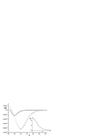
Figure 2: The average $\Delta H$ at an elementary time step (0.001 of a unit time) as a function of the angle $\phi$ between the patches. While a simple phase space random walk yields on average positive $\Delta H$, this property is shown here to hold only for small $\phi$. At larger angles, the diffusion between patches forces the system toward the center and the average $\Delta H$ becomes negative. Results are shown for $\Delta=0.1$ (full line) and $\Delta=1$ (dashed line). The inset shows the probability distribution function for $H$ at these two noise levels.

In conclusion, we suggest a novel solution to a long-standing conundrum: the stabilization of a noisy unstable dynamical system on spatial domains. The basic feature that leads to stabilization is the dependence of angular velocity on phase space coordinates. This dependence allows the noise to desynchronize spatially-coupled patches, and then migration decreases concentration gradients and leads to stabilization of a soft limit cycle close to the homogenous manifold. Clearly, owing to the phase space confinement of the trajectories, the exact nature of the noise becomes quite irrelevant, and thus our conclusions are also applicable to multiplicative noise (individual based dynamics). Furthermore, the effect of rare events - the trapping of the dynamics in the absorbing state for any finite system - should vanish in the thermodynamic limit, and thus one may expect a parametric dependent phase transition in that limit.

Appendix A The noisy Lotka-Volterra model

The Lotka-Volterra predator-prey system is a paradigmatic model for oscillations in population dynamics lotka ; volterra ; murray . It describes the time evolution of two interacting populations: a prey ($b$) population that grows with a constant birth rate $\sigma$ in the absence of a predator (the energy resources consumed by the prey are assumed to be inexhaustible), while the predator population ($a$) decays (with death rate $\mu$), in the absence of a prey. Upon encounter, the predator may consume the prey with a certain probability. Following a consumption event, the predator population grows and the prey population decreases. For a well-mixed population, the corresponding partial differential equations are:

$$\frac{\partial a}{\partial t} = -\mu a+\lambda_{1}ab$$ (2)

$$\frac{\partial b}{\partial t} = \sigma b-\lambda_{2}ab$$

where $\lambda_{1}$ and $\lambda_{2}$ are the relative increase (decrease) of the predator (prey) populations due to the interaction between species, correspondingly.

The system admits two unstable fixed points: the absorbing state $a=b=0$ and the state $a=0,\ \ b=\infty$. There is one marginally stable fixed point at $\bar{a}=\sigma/\lambda_{2},\ \ \bar{b}=\mu/\lambda_{1}$. Local stability analysis yields the eigenvalues $\pm i\sqrt{\mu\sigma}$ for the stability matrix. Moreover, even beyond the linear regime there is neither convergence nor repulsion. Using logarithmic variables $z=ln(a),\ q=ln(b)$ eqs. (2) take the canonical form $\dot{z}=\partial H/\partial q,\ \ \dot{q}=-\partial H/\partial z$, where the conserved quantity $H$ (in the $ab$ representation) is:

$$H=\lambda_{1}b+\lambda_{2}a-\mu\ ln(a)-\sigma\ ln(b).$$ (3)

The phase space, thus, is segregated into a collection of nested one-dimensional trajectories, where each one is characterized by a different value of $H$, as illustrated in Figure 3. Given a line connecting the fixed point to one of the ”walls” (e.g., the dashed line in the phase space portrait, Figure 3), $H$ is a monotonic function on that line, taking its minimum $H_{min}$ at the marginally stable fixed point (center) and diverging on the wall. Without loss of generality, we employ hereon the symmetric parameters $\mu=\sigma=\lambda_{1}=\lambda_{2}=1$. The corresponding phase space, along with the dependence of $H$ on the distance from the center and a plot of the oscillation period vs. $H$, are represented in Figure 3).

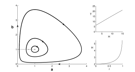
Figure 3: The Lotka-Volterra phase space (left panel) admits a marginally stable fixed point surrounded by close trajectories (three of these are plotted). Each trajectory corresponds to single $H$ defined in Eq. (3), where $H$ increases monotonically along the (dashed) line connecting the center with the $a=0$ wall, as shown in the lower right panel. In the upper right panel, the period of a cycle $T$ is plotted against $H$, and is shown to increase almost linearly from its initial value $T=2\pi/\sqrt{\mu\sigma}$ close to the center.

Given the integrability of that system, the effect of noise is quite trivial: if $a$ and $b$ randomly fluctuate in time (e.g., by adding or subtracting small amounts of population during each time step), the system wanders between trajectories, thus performing some sort of random walk in $H$ with ”repelling boundary conditions” at $H_{min}$ and ”absorbing boundary conditions” on the walls (as negative densities are meaningless, the ”death” of the system is declared when the trajectory hits the zero population state for one of the species). This result was emphasized by Gillespie gillaspee for the important case where intrinsic stochastic fluctuations are induced by the discrete character of the reactants. In that case, the noise is multiplicative (proportional to the number of particles), and the system flows away from the center and eventually hits one of the absorbing states at $0,0$ or $0,\infty$. The corresponding situation for a single patch Lotka-Volterra system with additive noise is demonstrated in Figure 4, where the survival probability $Q(t)$ (the probability that a trajectory does not hit the absorbing walls within time $t$) is shown for different noise amplitudes.

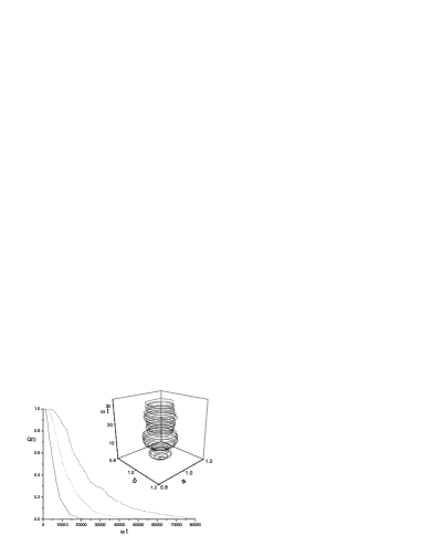
Figure 4: The survival probability $Q(t)$ is plotted versus time for a single patch noisy LV system. Eqs. (2) (with the symmetric parameters) were integrated numerically (Euler integration with time step $0.001$), where the initial conditions are at the fixed point $a=b=1$. At each time step, a small random number $\eta(t)\Delta t$ was added to each population density, where $\eta(t)\in[-\Delta,\Delta]$. A typical phase space trajectory, for $\Delta=0.5$, is shown in the inset. The system ”dies” when the trajectory hits the walls $a=0$ or $b=0$. Using 300 different noise histories, the survival probability is shown here for $\Delta=0.5$ (full line), $\Delta=0.3$ (dotted line) and $\Delta=0.25$ (dashed line). Clearly, the survival probability decays exponentially at long times, $Q(t)\sim exp(-t/\tau)$. As expected for a random walk with absorbing boundary conditions, $1/\tau$ scales with $\Delta^{2}$.

Appendix B Coupled oscillators

The Lotka-Volterra system (Appendix A) is somewhat complicated, since the angular velocity depends not only on $H$, but also on the location along a trajectory. In order to simplify the discussion, let us introduce a toy model that imitates the main features of the real systems. Although that model does not allow for an absorbing state, we believe that it captures the basic mechanism for stabilization of spatially extended systems in the presence of noise.

The toy model deals with the phase space behavior of diffusively coupled oscillators, where the angular frequency depends on the radius of oscillations. With additive noise, the Langevin equations take the form:

$$\frac{\partial x_{1}}{\partial t} = \omega(x_{1},y_{1})y_{1}+D_{1}(x_{2}-x_{1})+\eta_{1}(t)$$

$$\frac{\partial x_{2}}{\partial t} = \omega(x_{2},y_{2})y_{2}+D_{1}(x_{1}-x_{2})+\eta_{2}(t)$$

$$\frac{\partial y_{1}}{\partial t} = -\omega(x_{1},y_{1})x_{1}+D_{2}(y_{2}-y_{1})+\eta_{3}(t)$$ (4)

$$\frac{\partial y_{2}}{\partial t} = -\omega(x_{2},y_{2})x_{2}+D_{2}(y_{1}-y_{2})+\eta_{4}(t).$$

where all the $\eta$-s are taken from the same distribution. If the angular frequency is location independent, $\omega(x,y)=\omega_{0}$, the problem is reduced to coupled harmonic oscillators, a diagonalizable linear problem that admits two purely imaginary eigenvalues in the invariant, homogenous manifold. With the addition of noise, the random walk on that manifold is independent of the motion in the fast manifold, such that the radius of oscillation diverges with the square root of time. As there are no ”absorbing walls” here, the oscillation amplitude will grow indefinitely in the presence of noise.

Now let us define the oscillation radius for each patch, $r_{i}=\sqrt{x_{i}^{2}+y_{i}^{2}}$ for $i=1,2$, and assume that the angular frequency depends only on that radius and is $\theta$-independent [$\theta_{i}\equiv arctg(y_{i}/x_{i})$]. With that, the total phase $\Phi=\theta_{1}+\theta_{2}$ decouples and the 3-dimensional phase space motion is dictated by the equations (we assume $D_{1}=D_{2}=D$ and define $\phi=\theta_{1}-\theta_{2}$):

$$\dot{r_{1}} = -D(r_{1}-r_{2}\cos(\phi))+\tilde{\eta}_{1}(t)$$ (5)

$$\dot{r_{2}} = -D(r_{2}-r_{1}\cos(\phi))+\tilde{\eta}_{2}(t)$$

$$\dot{\phi}=- D \left(\frac{r_{1}^{2}+r_{2}^{2}}{r_{1}r_{2}}\right)sin\phi-\left[\omega(r_{1})-\omega(r_{2})\right]+\left(\frac{\tilde{\eta}_{3}}{r_{1}}-\frac{\tilde{\eta}_{4}}{r_{2}}\right).$$

As before, all the $\tilde{\eta}$-s are taken from the same distribution. In the harmonic limit, $\omega(r_{1})=\omega(r_{2})=\omega_{0}$, the only noisy term for $\phi$ vanishes at large $r$-s, and thus $\phi$ approaches zero. Defining now the new coordinates, $R\equiv r_{1}+r_{2}$, $r\equiv r_{1}-r_{2}$,

$$\dot{R}=-2Dsin^{2}(\phi/2)R+\eta$$ (6)

$$\dot{r}=-2Dcos^{2}(\phi/2)r+\eta,$$ (7)

one notices that at the limit $\phi=0$ the ”restoring force” in the $R$ direction vanishes and the phase space admits an attracting 1d-manifold $\phi=r=0$ (the invariant manifold). The noise, thus, induces random walk on that $R$ manifold, and since the walker cannot cross the origin, its displacement grows like $\sqrt{t}$.

Figure 5: Histograms showing the probability to be at a distance $R$ from the origin as a function of $R$, for two coupled noisy oscillators, where $\omega=1+\alpha r$ with $D=0.01$ and various values of noise strength $\Delta$ and angular velocity gradient $\alpha$. As expected, the phase space confinement is proportional to $\alpha$, from $\alpha=1$ (triangles) to $\alpha=0.5$ (circles) to $\alpha=0.1$ (solid line), all for the same level of noise $\Delta=0.1$. On the other hand, as predicted by the linear analysis close to the invariant manifold, the confinement is noise independent, and the three solid lines corresponding to different levels of noise ($\Delta=0.1,0.5,1$ with the same $\alpha=0.1$ almost coincide. The inset shows the flow lines on the $r=0$ plane. The invariant manifold $\phi=0$ is stable, but there is a ”maximally desynchronized” unstable orbit converging to the center at $\phi=\pi$. If the expectation value of $\phi^{2}$ deviates from zero, there is an effective restoring force toward the center, and the noise-induced random walk on the $\phi=0$ manifold is bounded.

In the generic case, however, where $\omega$ depends on $r$, the system behaves quite differently: if $r_{1}\neq r_{2}$, the two patches oscillate with different radial distance and desynchronize, i.e., $\langle\phi^{2}\rangle$ acquires, on average, some finite value. Migration, then, acts as a restoring force for an overdamped harmonic oscillator [Eq. (6)] and stabilizes the oscillations (if diffusion stabilizes the unstable fixed point this (noise independent) phenomenon is known as ”oscillation death” bareli ).

Following Eq. (6), close to the homogenous manifold (large diffusion, small noise limit), $r^{2}$ typical fluctuation around zero is of order $\Delta^{2}/D$. The $\omega(r_{1})-\omega(r_{2})$ term induces finite noise in the $\phi$ equation of motion, and thus $\langle\phi^{2}\rangle\sim(\omega^{{}^{\prime}}(r))^{2}\Delta^{2}/D^{3}$. This desynchronization, in turn, leads to the appearance of a finite restoring force on the invariant manifold $R$, as $\langle\phi^{2}\rangle\neq 0$, thus (far from the origin) one finds $\langle R^{2}\rangle\sim D^{2}/\omega^{{}^{\prime}}(r))^{2}$. The small $D$ instability (decoupled patches) manifest itself in the divergence of $r^{2}$ as $D\to 0$. It should be noted that, since both the restoring force and the noise in the invariant manifold are proportional to $\Delta^{2}$, the expected $R$ distribution has to be noise independent at that limit, as demonstrated in Figures 5 and 2. All in all, if $\omega$ is radius dependent, the coupled oscillators’ system stabilizes at some finite radius from the origin, giving rise to a soft ”limit cycle” in the 4-dimensional phase space, as indicated in Figure 5. The above considerations are valid only close to the homogenous manifold. For stronger noise, although the qualitative features of the system are the same, it was shown recently that mckane the effect of noise may shift the ”intrinsic” frequency of the system, leading to some shift of the intrinsic frequency.

Eqs. (B) may be generalized to include the case of an unstable focus (in order to imitate the dynamics of the Nicholson-Bailey bailey map) by adding a diagonal repulsive term to any variable (e.g., $\dot{x_{1}}=\omega(x_{1},y_{1})y_{1}+D_{1}(x_{2}-x_{1})+\eta_{1}(t)+\epsilon x_{1}$, where $\epsilon$ measures the ”strength” of the repulsion). The same analysis shows that, for small noise and small repulsion, a noise-induced transition will occur at $\epsilon\sim(\omega^{\prime 2}\ \Delta^{2}/D^{2})$. If the noise is small enough, the desynchronization is weak and cannot stabilize a soft limit cycle, and thus the system is, for real populations, extinction-prone. Strong noise, conversely, stabilizes the system and ensures species conservation.

References

- (1) Cuddington K. The ”balance of nature” methaphore and equilibrium in population ecology. Biology and Philosophy 16, 463-479 (2001).
- (2) Lotka A.J. Analytical note on certein rythmic relations in organic systems. Proc. Natl. Acad. Sci. USA 6, 410-415 (1920).
- (3) Volterra V. Variations and fluctuations of the numbers of individuals in anymal species living together. Lecon sur la Theorie Mathematique de la Lutte pour le via, Gauthier-Villars, Paris, 1931.
- (4) J.D. Murray, Mathematical Biology (Springer-Verlag, New-York, 1993).
- (5) Nicholson, A.J., Bailey, V.A. The balance of animal populations. Proc. Zool. Soc. London Part I 3, 551 598 (1935).
- (6) Nicholson, A.J., 1933. The balance of animal populations. J. Anim. Ecol. 2, 132 178 (1933).
- (7) Kerr B. et. al. Local migration promote competitive restraint in a host-pathogen ’tragedy of commons’. Nature 442, 75-78 (2006).
- (8) Holyoak M. & Lawler S.P., Persistence of an extinction prone predator-prey interaction through metapopulation dynamics. Ecology 77, 1867-1879 (2000).
- (9) Earn D.J.D., Levin S.A. & Rohani P. Coherence and conservation, Science 290, 1360-1363 (2000).
- (10) Blasius B., Huppert A. & Stone L. Complex dynamics and phase synchronization in spatially extended ecological systems, Nature 399, 354-359 (1999).
- (11) Gillespie D. T. Exact stochastic simulation of coupled chemical reactions. Journal of Physical Chemistry, 81, 2340 (1977).
- (12) Gause G.F. The struggle for existance. William and Wilkins, Baltimore (1934).
- (13) Luckinbill L.S. The effect of space and enrichment on a predator-prey system. Ecology 1142-1147 (1974).
- (14) Briggs C.J. & Hoopes M.F. Stabilizing effects in spatial parasitoid-host and predator-prey models: a review. Theoretical Population Biology 65, 299-315 (2004).
- (15) Allen, J.C. Mathematical models of species interactions in space and time. Am. Nat. 109, 319-342 (1975).
- (16) Reeve, J.D. Stability, variability, and persistence in host parasitoid systems. Ecology 71, 422-426 (1990).
- (17) Crowley, P.H. Dispersal and the stability ofpredator prey interactions. Am. Nat. 118, 673-701 (1981).
- (18) Jansen, V.A.A. Regulation of predator prey systems through spatial interactions: a possible solution to the paradox of enrichment. Oikos 74, 384-390 (1995).
- (19) Murdoch, W.W., Oaten, A. Predation and population stability. Adv. Ecol. Res. 9, 1-131 (1975)
- (20) Murdoch, W.W., Briggs, C.J., Nisbet, R.M., Gurney, W.S.C., Stewart- Oaten, A. Aggregation and stability in metapopulation models. Am. Nat. 140, 41-58 (1992).
- (21) Hassell, M.P., May, R.M.. Spatial heterogeneity and the dynamics ofparasitoi d host systems. Ann. Zool. Fenn. 25, 55-62 (1988).
- (22) Wilson, W.G., de Roos, A.M., McCauley, E. Spatial instabilities within the diffusive Lotka Volterra system: individual-based simulation results. Theor. Popul. Biol. 43, 91-127 (1993).
- (23) Bettelheim E., Agam O. & Shnerb N.M. ”Quantum phase transitions” in classical nonequilibrium processes. Physica E 9, 600 (2000).
- (24) Washenberger M.J., Mobilia M. & Tuber U.C. Influance of local carrying capacity restrictions on stochastic predator-prey models. cond-mat 0606809 (2006).
- (25) Donalson, D.D., Nisbet, R.M. Population dynamics and spatial scale: effects of system size on population persistence. Ecology 80, 2492-2507 (1999).
- (26) Bar-Eli K. On the stability of coupled chemical oscillators, Physica D 14 242 (1985).
- (27) McKane A.J. and Newman T.J. Predator-prey cycles from resonant amplification of demographic stochastisity, Phys. Rev. Lett. 94, 218102 (2005).