Quantum World-line Monte Carlo Method with Non-binary Loops and Its Application

Abstract

A quantum world-line Monte Carlo method for high-symmetrical quantum models is proposed. Firstly, based on a representation of a partition function using the Matsubara formula, the principle of quantum world-line Monte Carlo methods is briefly outlined and a new algorithm using non-binary loops is given for quantum models with high symmetry as SU($N$). The algorithm is called non-binary loop algorithm because of non-binary loop updatings. Secondary, one example of our numerical studies using the non-binary loop updating is shown. It is the problem of the ground state of two-dimensional SU($N$) anti-ferromagnets. Our numerical study confirms that the ground state in the small $N(\leq 4)$ case is a magnetic ordered Neel state, but the one in the large $N(\geq 5)$ case has no magnetic order, and it becomes a dimer state.

1 Introduction

The quantum world-line Monte Carlo (QMC) method has a long history. It has been used in many numerical studies of condensed-matter physics since it first proposed in 1970’s Suzuki1976 . However QMC simulations suffered as the result of some defects in conventional QMC algorithms. For example, near a critical point, or at low temperatures, the correlation time in samples became extremely long, thus we could not calculate the canonical ensemble average with accuracy. There were same problems in the Monte Carlo simulation of a classical system. Fortunately, a new algorithm was proposed by Swendsen and Wang, which solves such problems in classical systems. It is called cluster algorithm. The idea of the cluster algorithm can apply to quantum cases. Indeed, Evertz, Lana and Marcu first proposed a new QMC algorithm based on the cluster algorithm, which called loop algorithm EvertzLM1993 . The loop algorithm evolves into recent powerful QMC algorithms (See reviews Evertz2003 and KawashimaH2004 ).

In the present article, we will focus to the loop algorithm and the generalization for high-symmetrical quantum models. In Sect. 2, a useful representations of a partition function for recent QMC algorithms will be derived. In Sect. 3, the principle of QMC method and the detail of the loop algorithm will be reviewed. In Sect. 4, our generalization of the loop algorithm to a non-binary loop updating will be proposed. In Sect. 5, we will show one example of our numerical studies with the non-binary loop updating: the problem of the ground state of the two-dimensional SU($N$) quantum anti-ferromagnets.

2 World-line Representations Based on the Matsubara Formula

A density operator has all informations of a quantum system in an environment. In particular, if the system is in the heat-bath whose inverse temperature is $\beta$, the density operator $\rho(\beta)$ is the exponential operator of the system Hamiltonian as $\rho(\beta)=\exp(-\beta{\cal H})$, where ${\cal H}$ is the Hamiltonian of a quantum system.

The Hamiltonian usually consists of two parts ${\cal H}_{0}$ and $V$. Here ${\cal H}_{0}$ and $V$ denote diagonal and non-diagonal operators, respectively. The $V$ generally represents a perturbation part of the Hamiltonian. Then the non-trivial part of the density operator, $\rho^{\prime}(\beta)$, satisfies a special Bloch equation in which there is explicitly only the $V$ operator:

$$\frac{\mathrm{d}\rho^{\prime}(\beta)}{\mathrm{d}\beta}=-V(\beta)\rho^{\prime}(\beta)\qquad\left(\rho(\beta)\equiv\mathrm{e}^{-\beta({\cal H}_{0}+V)}\equiv\mathrm{e}^{-\beta{\cal H}_{0}}\rho^{\prime}(\beta)\right),$$ (1)

where $V(t)$ denotes the interaction picture of $V$ operator as $V(t)\equiv\mathrm{e}^{t{\cal H}_{0}}V\mathrm{e}^{-t{\cal H}_{0}}$. The solution of (1) formally satisfies an integral equation as

$$\rho^{\prime}(\beta)=I-\int_{0}^{\beta}\mathrm{d}tV(t)\rho^{\prime}(t),$$ (2)

where an integral variable $t$ is called imaginary time, because the Bloch equation is related to the Schrödinger equation through analytic continuation.

The solution of (2) is written as a series of multiple integrals of the product of interaction pictures of $V$:

$$\rho^{\prime}(\beta)=I-\int_{0}^{\beta}\mathrm{d}t_{1}V(t_{1})+\int_{0}^{\beta}\mathrm{d}t_{2}\int_{0}^{t_{2}}\mathrm{d}t_{1}V(t_{2})V(t_{1})-\cdots.$$ (3)

This representation of a density operator is known as the Matsubara formula. The order of interaction pictures $V(t)$ is in descending order. Since the perturbation part $V$ is usually the sum of local interaction Hamiltonians $V_{b}$, the density operator is a series of multiple integrals of the product of interaction pictures of $V_{b}$:

$$\rho(\beta)=\mathrm{e}^{-\beta{\cal H}_{0}}\sum_{n=0}^{\infty}\mathop{\sum}_{b_{n},\cdots,b_{1}}\mathop{\int}_{\beta\geq t_{n}\geq\cdots\geq t_{1}\geq 0}\mathrm{d}t_{n}\cdots\mathrm{d}t_{1}(-1)^{n}V_{b_{n}}(t_{n})\cdots V_{b_{1}}(t_{1}),$$ (4)

where $V=\sum_{b}V_{b}$.

The matrix element of operator $AB$ is equal to the summation of products of each matrix elements of $A$ and $B$.

$$\langle\Psi_{A}|AB|\Psi_{B}\rangle=\sum_{\{|\psi\rangle\}\mbox{:basis}}\langle\Psi_{A}|A|\psi\rangle\langle\psi|B|\Psi_{B}\rangle,$$ (5)

where the set $\{|\psi\rangle\}$ is an orthonormal basis in the quantum state space. Therefore, inserting an orthonormal basis $\{|\psi\rangle\}$ between two operators of integrand in the Matsubara formula, the partition function $Z$ can be represented as a multiple integral with respect to three kinds of variables, $\psi_{i},\ b_{i}$ and $t_{i}$:

$$Z \equiv \mathrm{Tr}\rho(\beta)$$ (6)

$$= \sum_{n=0}^{\infty}\mathop{\sum}_{\psi_{n},\cdots,\psi_{1}(\psi_{n+1}=\psi_{1})}\mathop{\sum}_{b_{n},\cdots,b_{1}}\mathop{\int}_{\beta\geq t_{n}\geq\cdots\geq t_{1}\geq 0}W_{n}(\{\psi_{i}\},\{b_{i}\},\{t_{i}\}),$$ (8)

$$W_{n}(\{\psi_{i}\},\{b_{i}\},\{t_{i}\})\equiv\mathrm{e}^{-\beta{\cal H}_{0}(\psi_{1})}\prod_{i=1}^{n}\langle\psi_{i+1}|\{-V_{b_{i}}(t_{i})\mathrm{d}t_{i}\}|\psi_{i}\rangle,$$

where ${\cal H}_{0}(\psi_{1})\equiv\langle\psi_{1}|{\cal H}_{0}|\psi_{1}\rangle$.

The status of a variable set $(\{\psi_{i}\},\{b_{i}\},\{t_{i}\})$ is called world-line configuration, because it can be represented as a set of world-lines. Figure 1 shows a world-line configuration of an $s=1/2$ Heisenberg anti-ferromagnet (HAF) model on a four-sites chain.

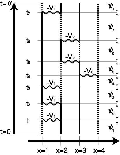
Figure 1: A graphical representation of a world-line configuration for an $s=1/2$ Heisenberg anti-ferromagnet model on a four-sites chain. Solid and dotted lines denote spin states $+\frac{1}{2}$ and $-\frac{1}{2}$, respectively. A position of a waiving line corresponds to the status of a variable set $(b_{i},t_{i})$.

The X axis refers the position of spin sites, from 1 to 4, and the Y axis refers the imaginary time, from 0 to $\beta$. In this example, the Hamiltonian consists of local interaction Hamiltonians $V_{1}$, $V_{2}$ and $V_{3}$. The $V_{b}$ is the Hamiltonian of the HAF interaction between sites $b$ and $b+1$. Then a waving line is drawn at the position corresponding to the status of $(b_{i},t_{i})$. The vertical line denotes the status of $\psi_{i}$ between two $V_{b}$. In the $s=1/2$ case, we need two line types, for example, solid and dotted lines which denote up and down spin states of an $s=1/2$ spin, respectively. In this way, this figure is in one-to-one correspondence with the world-line configuration. Usually, the waving line is called vertex and the position at where a local spin configuration changes is called kink. Since we will only show examples of quantum spin models in the present article, the status of variables $\psi_{i}$ is called spin configuration.

From (8), the function $W_{n}$ can be regarded as the Boltzmann weight of a world-line configuration. Therefore, using the Matsubara formula, the partition function can be transformed from quantum to classical one.

3 Quantum World-line Monte Carlo Method

Using the same technique for the partition function, we can get a similar multiple integral representation of a canonical ensemble average of an observable A.

$$\langle A\rangle\equiv\frac{\mathrm{Tr}A\rho(\beta)}{Z}=\sum_{(\{\psi_{i}\},\{b_{i}\},\{t_{i}\})}A(\psi_{1})\frac{W_{n}(\{\psi_{i}\},\{b_{i}\},\{t_{i}\})}{Z},$$ (9)

where $A(\psi_{1})\equiv\langle\psi_{1}|A|\psi_{1}\rangle$. Here the symbol $\sum_{(\{\psi_{i}\},\{b_{i}\},\{t_{i}\})}$ denotes the multiple integral for variables $(\{\psi_{i}\},\{b_{i}\},\{t_{i}\})$. In other words, we sum up with respect to all world-line configurations.

Since $\sum_{(\{\psi_{i}\},\{b_{i}\},\{t_{i}\})}W_{n}=Z$, the function $W_{n}/Z$ in (9) can be regarded as the probability of a world-line configuration. Therefore, if we can sample a world-line configuration with the probability $W_{n}/Z$, the canonical ensemble average $\langle A\rangle$ can be calculated as the average of samples of the function $A(\psi_{1})$. This is the principle of the QMC method.

Many algorithms have been proposed to make a sample of world-line configurations. However the conventional algorithm before the loop algorithm suffered from some problems. In general, since the probability distribution of world-line configurations is complex, a sampling algorithm of world-line configurations is based on a Markov process. Samples in a Markov process are usually correlated for some time steps which is called correlation time. Unfortunately the correlation time in the conventional sampling algorithm becomes very large near a critical point and at low temperatures, because the size of an updating unit of a world-line configuration is fixed when the correlation length of a quantum system increases. Therefore it is difficult to calculate a canonical ensemble average of a quantum system at interesting points using the conventional algorithm.

3.1 Loop Algorithm

The loop algorithm is one of recent developed QMC algorithms. It uses a geometrical object which called loop and updates a world-line configuration with loops globally. For some important quantum models, we can prove that the size of loop in the loop algorithm is equal to the correlation length of the quantum model. This is the reason why the loop algorithm will avoid problems in QMC simulations. In fact, the loop algorithm has some good properties as follows. The first good property is that the correlation time in samples is very short at a critical point and low temperatures. The second one is that various types of world-line configurations can be sampled naturally, which called grand canonical sampling. In practice, it is difficult to change the value of an order parameter without artificial techniques in the conventional algorithm.

The procedure of a loop algorithm consists of three steps. Figure 2 illustrates these steps for an $s=1/2$ HAF model on a four-sites chain.

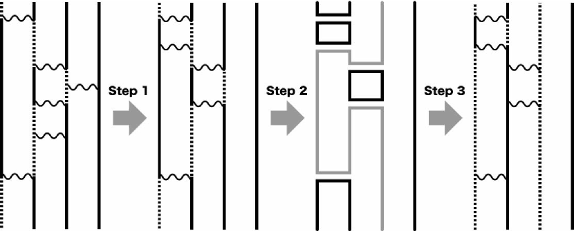
Figure 2: A loop updating for an $s=1/2$ Heisenberg anti-ferromagnet model on a four-sites chain. Solid and dotted line denote spin states $+\frac{1}{2}$ and $-\frac{1}{2}$, respectively. The gray loop in the third sub-figure is only flipped.

The first step is to update vertexes. In this step, the number of vertexes is changed and those positions are moved, but the spin configuration is fixed. We separately update vertexes and the spin configuration. The second step is to decompose spin variables into loops. In Fig. 2 they are decomposed into five loops. The third step is to flip each loop with a probability $1/2$. The flipping of a loop is to change the sign of spin variables on the loop. In the quantum $s=1/2$ spin model, a basis of a quantum state space can be made of the direct product of two states, up and down states, on each spin site. Thus a spin variable takes only two values as $\pm 1/2$ and it can be flipped. Although the gray loop in Fig. 2 is only flipped, the spin configuration is drastically changed to the right one. Since there are great differences between the initial and the final world-line configurations, the correlation time of a loop algorithm is very short.

Since the sampling distribution defined by the weight of a world-line configuration is very complex and the partition function is unknown in advance, we use the Markov process whose equilibrium distribution of configurations is equal to the desired sampling distribution. In order to make the Markov process, it is enough to satisfy the detail balance condition for any two configurations A and B in the Markov process:

$$W({\mathrm{A}})P({\mathrm{A}}\to{\mathrm{B}})=W({\mathrm{B}})P({\mathrm{B}}\to{\mathrm{A}}),$$ (10)

where $W(\cdot)$ is the weight function of a desired distribution and $P({\mathrm{A}}\to{\mathrm{B}})$ is the transfer probability from A to B. In other words, the density of random walkers is controlled through their transfer probabilities which balance with the desired sampling distribution. In the loop algorithm, two updatings for vertexes and spin configurations are alternately done and each transfer probability satisfies the detail balance condition.

Firstly, the updating of vertexes is considered. If a vertex $V_{b}$ is inserted at an imaginary time $t$ between $t_{k+1}$ and $t_{k}$ ($t_{k+1}\geq t\geq t_{k}$), the weight of a new world-line configuration $W_{n+1}$ is equal to the present one ($W_{n}$ in (8)) multiplied by a matrix element of $V_{b}$ with $\mathrm{d}t$: $\langle\psi_{k+1}|\{-V_{b}(t)\mathrm{d}t\}|\psi_{k+1}\rangle$. The ratio of two weights of pre- and post-inserted a vertex $V_{b}$ between the imaginary time $t$ and $t+\mathrm{d}t$ is proportional to the infinitesimal $\mathrm{d}t$. Therefore, from (10), the accept probability of the inserting of the vertex is proportional to the infinitesimal $\mathrm{d}t$. Such stochastic process is called Poisson process. Scanning a world-line configuration with the Poisson process, we can insert vertexes under the detail balance condition. The thing to do next is to remove a vertex. If a vertex is not on a kink, the ratio of weights between pre- and post-removed configurations is infinite. From (10), we can always remove a vertex on a non-kink. On the other hand, if a vertex is on a kink, the ratio of them is exactly zero. Thus it can not be can removed. In summary, the stochastic inserting process of vertexes is a Poisson process whose intensity is equal to a matrix element of a vertex. And the removing a vertex must be done if and only if the vertex is not on a kink.

This updating procedure of vertexes by a Poisson process is applicable to various quantum models, and it is employed in various QMC algorithms. However, on the contrary, it is difficult to find an efficient updating of a spin configuration because of the interaction of spin variables thorough vertexes. In particular, the weight of random generated spin configurations is usually equal to zero, because the matrix element of each vertex often takes a value 0. Thus we need an ingenious updating procedure.

Fortunately, it has been found for some important quantum models. In such cases, the interaction Hamiltonian takes the special form which is called delta operator. The delta operator is defined as the matrix element taking only a value 0 or 1. For example, the HAF interaction Hamiltonian is equal to a special delta operator $\hat{\Delta}(g_{H})$ divided by 2 with a special unitary transformation:

$$-{\cal H}_{ij}^{\mathrm{HAF}}\equiv-U^{-1}\left(\vec{S}_{i}\cdot\vec{S}_{j}-\frac{1}{4}\right)U=\frac{1}{2}\hat{\Delta}(g_{H}).$$ (11)

Furthermore, the condition of the matrix element taking a value 1 is as follows:

$$\langle\sigma_{i}^{\prime}\sigma_{j}^{\prime}|\hat{\Delta}(g_{H})|\sigma_{i}\sigma_{j}\rangle\equiv\left\{\begin{array}[]{cl}1&(\mbox{if}\ \sigma_{i}+\sigma_{j}=\sigma_{i}^{\prime}+\sigma_{j}^{\prime}=0)\\ 0&(\mbox{otherwise})\end{array}\right.,$$ (12)

where $\sigma_{i}(\sigma_{j})$ denotes a spin state on a site $i(j)$ and it takes an eigenvalue of an $s=1/2$ z-direction spin operator as $\sigma_{i}\equiv\pm\frac{1}{2}$.

The condition of taking a value 1 for a delta operator can be often represented by a graph. If a delta operator of an interaction Hamiltonian has the graphical representation, we can construct the loop algorithm on the quantum model. For example, the condition of the $\hat{\Delta}(g_{H})$ operator is simply represented by a horizontal graph in Fig. 3 (a). The horizontal dotted line in Fig. 3 (a) denotes the necessary condition: the sum of two connected spin variables must be equal to zero. From the definition, a matrix element of a delta operator takes only a value 0 or 1. Therefore the value of a vertex weight is not changed, as long as a modification of a spin configuration matches the graphical representation. In the horizontal graph, the modification of the two connected spin variables is only restricted, thus disconnected spin variables are not related to each other: $\sigma_{i}$ and $\sigma_{i}^{\prime}$. Furthermore, the flipping of two connected spin variables together is always allowed, because it satisfies the condition and the weight is not changed. Therefore, we can always flip each set of connected spin variables independently.

In summary, the procedure of updating a spin configuration consists of three steps. In the first step each vertex is replaced with a corresponding graph. The second step is to decompose spin variables into a set which defined by graphs. Since a set of connected spin variables always becomes a loop for the $s=1/2$ HAF model, this updating algorithm is called loop algorithm. The third step is to flip each loop or set randomly with a probability $\frac{1}{2}$. The loop takes one of two states, because the spin variable takes only a value $\pm\frac{1}{2}$ for the $s=1/2$ HAF model. Thus we call it binary loop.

The loop updating was very successful, because the size of loop is related to the physical correlation length of a quantum model. And by the loop algorithm, many important results were numerically found for various quantum models.

Although we showed only a quantum $s=1/2$ spin model, the loop updating is also applicable to quantum large spin models. For such cases, Kawashima and Gubernatis proposed a mapping to a quantum $s=1/2$ spin model which called split-spin technique KawashimaG1994 . The idea is that an $s=m$ spin operator is replaced by the sum of $2m$ $s=1/2$ spin operators with a permutation operator. Since they are isomorphic, we can simulate a quantum $s=m$ model as a multi quantum $s=1/2$ model with binary loop updatings. However, since the size of the new quantum space becomes large, we need more memories and complex treatments. In the next section, we will propose a new loop updating which acts on an original quantum space directly.

4 Non-binary Loop Algorithm

The symmetry of a model is related to the graphical representation of a vertex. For example, the HAF model has the SU(2) symmetry and the HAF interaction term is represented as the binary horizontal graph. Fortunately, there are such special graphical representations in high-symmetrical cases.

The $s=1$ bi-linear bi-quadratic (BLBQ) model is interesting theoretically and experimentally BIQ , because it has some integrable points for a one-dimensional case and it is related to the effective model of Na atoms in an optical lattice GreinerMEHB2002 . The Hamiltonian is as follows:

$${\cal H}_{ij}^{\mathrm{BLBQ}}\equiv(\cos\theta)\vec{S}_{i}\cdot\vec{S}_{j}+(\sin\theta)(\vec{S}_{i}\cdot\vec{S}_{j})^{2}.$$ (13)

The BLBQ model has SU(3) symmetry at special points, for example, $\theta=-\frac{\pi}{2}$ and $-\frac{3\pi}{4}$. The BLBQ interaction terms at SU(3) points have special graphical representations whose states are non-binary as 0 and $\pm 1$. For example, the BLBQ interaction term at the SU(3) point $\theta=-\frac{\pi}{2}$ becomes a delta operator and the condition taking a value 1 is same to that in an $s=1/2$ HAF case, except for a spin variable takes three values, $\pm 1$ and $0$. As a result, we can use the same horizontal graph in Fig. 3 (a) for the BLBQ interaction term. However, the loop, which defined by the SU(3) horizontal graph, takes three states, not binary states.

We can generalize the horizontal graph in the SU($N$) case. In the SU($N$) case, since the spin variable takes $N$ values ($\sigma_{i}=\frac{(-N+1)}{2},\cdots,\frac{(N-1)}{2}$), the number of loop states which defined by the SU($N$) horizontal graph is $N$. Thus we call it non-binary loop. Another type of graph can also be generalized in the SU($N$). For example, we found the generalized cross graph $g_{C}$ in Fig. 3 (b) which corresponds to the other SU(3) point $\theta=-\frac{3\pi}{4}$:

$$\langle\sigma_{i}^{\prime}\sigma_{j}^{\prime}|\hat{\Delta}(g_{C})|\sigma_{i}\sigma_{j}\rangle\equiv\left\{\begin{array}[]{cl}1&(\mbox{if}\ \sigma_{i}-\sigma_{j}^{\prime}=\sigma_{i}^{\prime}-\sigma_{j}=0)\\ 0&(\mbox{otherwise})\end{array}\right..$$ (14)

It is easy to check that generalized graphs have the SU($N$) symmetry.

The loop defined by the SU($N$) graph has $N$ possible states of equal weight, because the exchange of any two states corresponds to one of SU($N$) transformations. Therefore we can choose one of $N$ possible states for each loop with equal probability.

In summary, the procedure of the loop updating using the SU($N$) graph is similar to that of the conventional loop algorithm with the binary graph. In the first step each vertex is replaced by a corresponding SU($N$) graph. And the second step is to decompose spin variables into a set which defined by the SU($N$) graphs. In the third step we choose one of $N$ possible states for each set with equal probability. The only difference between the conventional and new loop algorithms is the number of possible loop states.

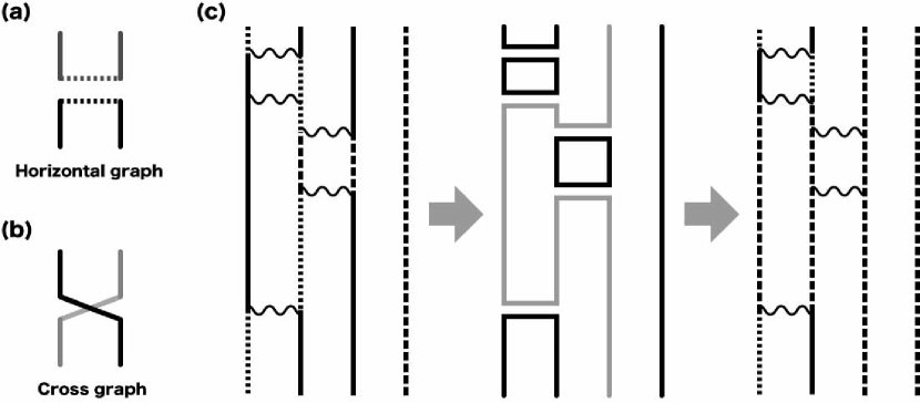
Figure 3: Graphs for various types of vertexes and a non-binary loop updating for an $s=1$ BLBQ model on a four-sites chain. (a) Horizontal graph. (b) Cross graph. (c) The non-binary loop updating for an $s=1$ BLBQ model at $\theta=-\frac{\pi}{2}$. Solid, dashed, and dotted lines denote the spin states, +1, 0, and -1, respectively. The gray loop in the second sub-figure is only changed.

The loop algorithm with non-binary loops is called non-binary loop algorithm KawashimaH2004 . It is very useful to study high-symmetrical quantum models, because of the simplicity. Without a split-spin technique, we can directly simulate the SU($N$) model in the original quantum space. The relation between the conventional and new loop algorithms is similar to that between Swendsen–Wang algorithms for Ising and Potts models.

5 Application: Ground States of Two-Dimensional SU($N$) Quantum Anti-ferromagnets

Some quantum models already have been simulated with the non-binary loop algorithm. In the present section, we will focus on the numerical study of ground states of two-dimensional SU($N$) quantum anti-ferromagnets.

The existence of a short-range resonating valence bond (RVB) spin-liquid is a very interesting problem for low-dimensional quantum systems. A RVB spin-liquid exhibits a finite gap for spin-excitations and it has only short-range order and it does not break any lattice symmetry. Although the RVB spin-liquid may be related to the mechanism of the copper-oxide superconductors, the ground state of the two-dimensional $s=1/2$ HAF model, which is an effective quantum spin model of copper-oxide superconductor, is not a RVB state, but it has a magnetic order which called Neel order. As the spin $s$ is decreased, the quantum fluctuation decreases the Neel order, but the ground state remains ordered even for $s=1/2$. Another route to increase quantum fluctuations is in the symmetry of quantum models. We studied the SU($N$) quantum anti-ferromagnets which is one of generalizations of the HAF model and which has the higher symmetry than SU(2).

Our Hamiltonian of SU($N$) quantum anti-ferromagnets is defined by the generator of SU($N$) algebra as the HAF model:

$${\cal H}_{ij}^{\mathrm{SU(}N\mathrm{)}} \equiv \frac{1}{N}\sum_{\alpha,\beta=1}^{N}J_{\beta}^{\alpha}(i)J^{\beta}_{\alpha}(j),$$ (15)

$$\left[J_{\beta}^{\alpha}(i),J^{\mu}_{\nu}(j)\right] = \delta_{ij}\left(\delta_{\nu}^{\alpha}J_{\beta}^{\mu}(i)-\delta_{\beta}^{\mu}J_{\nu}^{\alpha}(i)\right),$$ (16)

where $J_{\beta}^{\alpha}(i)$ is an SU($N$) generator on site $i$. In the SU(2) case, this Hamiltonian is equal to the HAF model. In our anti-ferromagnetic SU($N$) model, the representation of SU($N$) generator is a $N$-dimensional matrix which called fundamental representation and the matrix on one sub-lattice is conjugate to that on the other sub-lattice. In this representation, the model can be expressed in terms of SU(2) spins with $s=(N-1)/2$. If the SU($N$) Hamiltonian applies to the $|nm\rangle$ state, the result equals the superposition of all $|l\bar{l}\rangle$ states divided by $N$:

$${\cal H}_{ij}^{\mathrm{SU(}N\mathrm{)}}|nm\rangle=-\delta_{n\bar{m}}\left(\frac{1}{N}\sum_{l=-s,\cdots,s}|l\bar{l}\rangle\right)\equiv-\delta_{n\bar{m}}|(ij)\rangle.\quad(\bar{l}\equiv-l),$$ (17)

where $|nm\rangle$ denotes the simultaneous eigenstate of z-direction SU(2) spin operators on sites $i$ and $j$. For convenience, the special superposition state $|(ij)\rangle$ will be called $(ij)$-bond state in the following.

The $(12)$-bond state is a ground state of a two-sites case. And it has no magnetic order, because it is the superposition of different magnetic ordered states. In a four-sites case, a bond state $|(12)(34)\rangle$ is an eigenstate of ${\cal H}_{12}^{\mathrm{SU(}N\mathrm{)}}$ and ${\cal H}_{34}^{\mathrm{SU(}N\mathrm{)}}$ whose eigenvalue is -1. However, if the interaction Hamiltonian does not match the covering of dimers over sites in a bond state, the state converges to a zero-eigenstate when $N$ becomes infinity:

$${\cal H}_{23}^{\mathrm{SU(}N\mathrm{)}}|(12)(34)\rangle=-\frac{1}{N}|(41)(23)\rangle\to 0\quad(N\to\infty).$$ (18)

Therefore, in the large $N$ limit, the ground state maximizes the number of nearest-neighbor bonds, because the eigenvalue of a whole Hamiltonian is minus of the number of nearest-neighbor bonds. In short, in the large $N$ limit, due to strong quantum fluctuations, the ground state has no magnetic order. However, in a one-dimensional chain, the number of maximum bond state is only two Affleck1985 . Since they break the translational symmetry, they are not a RVB state, which called dimer state. Read and Sachdev studied the ground state of SU($N$) models on a two-dimensional square lattice theoretically ReadS1990 . Their conclusion is also that the ground state on a two-dimensional square lattice is a dimer state in the large $N$ limits.

In the $N=2$ case, the ground state is a magnetic ordered Neel state. On the other hand, in the large $N$ limit, it has no magnetic order and it becomes a dimer state by Read and Sachdev’s prediction. However the intermediate $N$ cases remain problems. The numerical study by Santoro et al. suggested a RVB spin-liquid ground state in the $N=4$ case Santoro1999 . The model of Santoro et al. is equal to our SU(4) model and it also appears as a special point in coupled spin-orbital models. Santoro et al. used the Green function Monte Carlo method in their numerical simulations. Due to the computational times by their numerical method, the size of their simulated lattices was limited to only $L=12$.

Since the SU($N$) interaction Hamiltonian is equal to the delta operator $\hat{\Delta}(g_{H})$ represented by the non-binary horizontal graph, this model can be simulated for various $N$ and large square lattices by a non-binary loop algorithm. Indeed, we explored the system size $L$ up to 128 and $N$ up to 8 HaradaK2003 . Our simulations have been performed at low enough temperatures to be effectively in the ground state. The lowest temperature for $N=4$ and $L=128$, for example, is $\frac{1}{128}$.

In order to search the order of a ground state, we have measured two quantities which are related to magnetic and dimer orders, respectively. The one is a static structure factor $S(\pi,\pi)$ of staggered magnetization $m_{s}$ and the other is a dimer static structure factor $S^{\mathrm{D}}(\pi,0)$:

$$\frac{S(\pi,\pi)}{L^{2}}\equiv\langle(m_{s})^{2}\rangle\qquad\qquad\quad\left(m_{s}\equiv\frac{1}{L^{d}}\sum_{r}(-1)^{r}S^{z}_{r}\right)$$ (19)

and

$$\frac{S^{\mathrm{D}}(\pi,0)}{L^{2}}\equiv\langle(d_{(\pi,0)})^{2}\rangle\ \quad\qquad\left(d_{(\pi,0)}\equiv\frac{1}{L^{d}}\sum_{r}(-1)^{r_{x}}S^{z}_{r}S^{z}_{r+x}\right).$$ (20)

If an order exists, the related structure factor divided by $L^{2}$ converges to a finite value in the large-$L$ limits, but if the order is absent, it decreases to zero as $1/L^{2}$.

Figure 4 shows a clear evidence for a Neel order in $N\leq 4$, because the spin structure factor divided by $L^{2}$ converges to a finite value for $N\leq 4$. Therefore the ground state is not a RVB spin-liquid even in the $N=4$ case. On the contrary, in the $N\geq 5$ cases, the spin structure factor divided by $L^{2}$ decreases as $1/L^{2}$. Therefore there is no Neel order in $N\geq 5$.

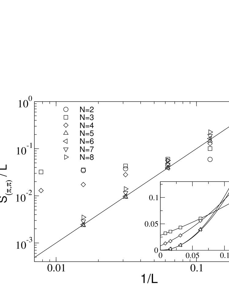
Figure 4: Static structure factors $S_{(\pi,\pi)}$ for $2\leq N\leq 8$. The straight line representing the power law $L^{-2}$ is drawn for comparison. Estimated statistical errors are not shown, because they are equal to or smaller than the symbol size. The inset presents the data for $N=3,4,5,6$ in the linear scale, together with the best fitting curves obtained by the method of least squares. (Adopted from Harada and Kawashima HaradaK2003 )

The disagreement of our conclusion for the $N=4$ case with that of Santoro et al. is not in the raw numerical data. Their data are only in the $L\leq 12$ region. Therefore, the disagreement is solely due to the small system sizes studied in Santoro1999 .

On the other hand, Fig. 5 shows a clear evidence for a dimer order in $N\geq 5$. While the dimer structure factor divided by $L^{2}$ decreases to zero in $N=4$, it converges to a finite value in $N\geq 5$. Therefore the dimer order exists in $N\geq 5$ and the ground state is not a RVB spin-liquid state. It is consistent with the theoretical prediction by Read and Sachdev in the large $N$ limits.

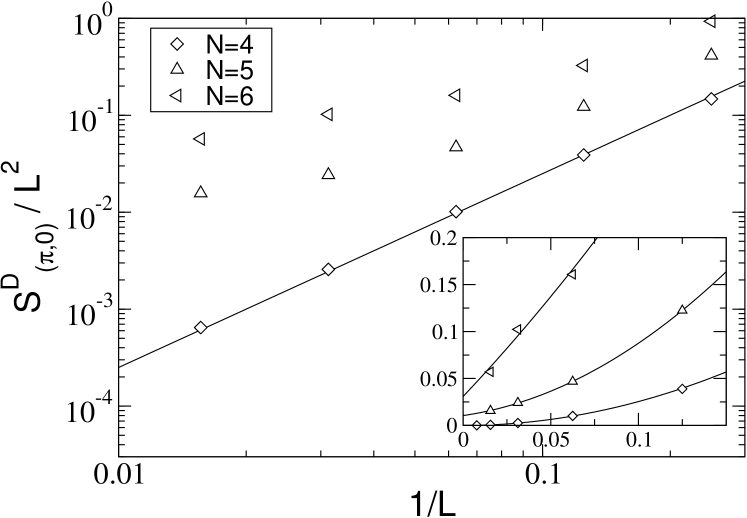
Figure 5: The ${\bf k}=(\pi,0)$ dimer structure factors $S_{(\pi,0)}^{\mathrm{D}}$ for $N=4,5,6$ in logarithmic scale. The inset is the linear-scale plot. The solid lines in the inset are the best fitting curves of least squares based on the $L\geq 8$ data. (Adopted from Harada and Kawashima HaradaK2003 )

In summary, from QMC simulations for large square lattices by the loop algorithm with non-binary loops, we confirmed a direct transition from the Neel ground state ($N\leq 4$) to the dimer ground state ($N\geq 5$) for two-dimensional SU($N$) quantum anti-ferromagnets. These comprehensive numerical studies can be effectively done by the loop algorithm with non-binary loops.

6 Conclusion

We have introduced the QMC method with non-binary updatings for quantum models with high symmetry. For example, using graphical representations of the interaction Hamiltonian, we can easily simulate a high-symmetrical quantum model by a loop algorithm with non-binary loops. We have only focused to the loop algorithm, but the idea of a non-binary updating for quantum models with high symmetry can be combined with the other algorithms as the worm or directed loop. We have shown one example for using a non-binary loop algorithm. It is the problem of the ground state of two-dimensional SU($N$) quantum anti-ferromagnets. Our conclusion is that our SU($N$) models have no RVB spin-liquid ground state.

References

- (1) M. Suzuki: Prog. Theor. Phys. 56 1454 (1976).
- (2) H. G. Evertz, G. Lana and M. Marcu: Phys. Rev. Lett. 70 875 (1993).
- (3) H. G. Evertz: Advances in Physics 52 1 (2003).
- (4) N. Kawashima and K. Harada: J. Phys. Soc. Jpn. 73 1379 (2004).
- (5) N. Kawashima and J. E. Gubernatis: Phys. Rev. Lett. 73 1295 (1994).
- (6) For physical results on this model, see, for example, A. Schmitt, K-H. Mütter, M. Karbach, Y. Yu, and G. Müller: Phys. Rev. B 58 5498 (1998), and references cited therein; also see K. Nomura and S. Takada: J. Phys. Soc. Jpn. 60 389 (1991).
- (7) M. Greiner, O. Mandel, T. Esslinger, T. W. Hănsch, and I. Bloch: Nature 415 39 (2002).
- (8) N. Read and S. Sachdev: Phys. Rev. B 42 4568 (1990).
- (9) I. Affleck: Phys. Rev. Lett. 54 966 (1985).
- (10) G. Santoro, S. Sorella, L. Guidoni, A. Parola, and E. Tosatti: Phys. Rev. Lett. 83 3065 (1999).
- (11) K. Harada and N. Kawashima: Phys. Rev. Lett. 90 117203 (2003).