Dynamic particle tracking reveals the aging temperature of a colloidal glass

Abstract

Understanding glasses is considered to be one of the most fundamental problems in statistical physics. A theoretical approach to unravel their universal properties is to consider the validity of equilibrium concepts such as temperature and thermalization in these out-of-equilibrium systems. Here we investigate the autocorrelation and response function to monitor the aging of a colloidal glass. At equilibrium, all the observables are stationary while in the out-of-equilibrium glassy state they have an explicit dependence on the age of the system. We find that the transport coefficients scale with the aging-time as a power-law, a signature of the slow relaxation. Nevertheless, our analysis reveals that the glassy system has thermalized at a constant temperature independent of the age and larger than the bath, reflecting the structural rearrangements of cage-dynamics. Furthermore, a universal scaling law is found to describe the global and local fluctuations of the observables.

Introduction.— Increasing the volume fraction of a colloidal system slows down the Brownian dynamics of its constitutive particles, implying a limiting density, $\phi_{g}$, above which the system can no longer be equilibrated with its bath Pusey . Hence, the thermal system falls out of equilibrium on the time scale of the experiment and thus undergoes a glass transition Cugliandolo . Even above $\phi_{g}$ the particles continue to relax, but the nature of the relaxation is very different to that in equilibrium. This phenomenon of a structural slow evolution beyond the glassy state is known as “aging” Struik . The system is no longer stationary and the relaxation time is found to increase with the age of the system, $t_{w}$, as measured from the time of sample preparation.

This picture applies not only to structural glasses such as colloids, silica and polymer melts, but also to spin-glasses, ferromagnetic coarsening, elastic manifolds in quenched disorder and jammed matter such as grains and emulsions Cugliandolo ; Kurchan_prl ; Bouchaud . Theories originally developed in the field of spin-glasses Kirkpatrick attempt to develop a common framework for the understanding of aging. For example, the structural glass and spin-glass transitions have been coupled by the low temperature extension of the Mode-Coupling Theory (MCT) Kurchan_MCT ; Kurchan_prl ; Bouchaud . More generally, this approach is related to analogous ideas developed in the field of granular matter such as compactivity Edwards ; Ono ; Makse_nature ; Anna ; Song , and the inherent structure formalisms Stillinger , adapted to the energy landscape of glasses Sciortino .

One of the important features of this scenario is a separation of time-scales where the observables are equilibrated at different temperatures, even though the system is far from equilibrium. While theoretical results have flourished, the difficulties in the experimental testing of the fundamental predictions of the theories have hampered the development of an understanding of aging in glasses Israeloff ; Bellon ; Herisson ; Buisson ; Abou . Experiments so far have shown conflicting results which are usually masked by large intermittent fluctuations in the observables Buisson ; a behavior which seems beyond the current theoretical formalisms Cugliandolo . On the other hand, some numerical results are more favorable Parisi ; Barrat_Kob ; Berthier . Furthermore, the concept of temperature has been shown to be useful to describe other far form equilibrium systems such as non-thermal granular materials Ono ; Makse_nature ; Anna ; Song .

Here we use a model glass which is one of the simplest systems undergoing a glass transition: a colloidal glass of micrometer size particles, where the interactions between particles can be approximated as hard core potentials Pusey ; Kegel ; Weeks_sci . The system is index matched to allow the visualization of tracer particles in the microscope Weeks_sci . Owing to the simplicity of the system, we are able to follow the trajectories of magnetic tracers embedded in the colloidal sample and use this information as an ideal “thermometer” to measure the temperature for the different modes of relaxation. In turn, we measure the autocorrelation function of the displacements and the integrated response to an external magnetic field as an indicator of the dynamics via a Fluctuation-Dissipation Theorem (FDT). For this system we show that, even though the diffusivities and mobilities of the tracers scale with the age of the system, there exists an effective temperature which is uniquely defined and remains constant independent of the age. This effective temperature is larger than the bath temperature and controls the slow relaxation of the system, as if the system were at “equilibrium”. We find a scaling behavior with the waiting time, which describes in a unified way not only the global but also the local fluctuations of the correlations and responses as well as the cage dynamics in the system.

Correlations and responses.— Our experiments use a colloidal suspension consisting of a mixture of poly-(methylmethacrylate) (PMMA) sterically stabilized colloidal particles (radius $a_{p}=1.5\ \mu m$, density $\rho_{p}=1.19\ g/cm^{3}$, polydispersity $\sim 14\%$) plus a small fraction of superparamagnetic beads (radius $a_{m}=1.6\ \mu m$ and density $\rho_{m}=1.3\ g/cm^{3}$, from Dynal Biotech Inc.) as the tracers (More details in the Method section). In order to investigate the dynamical properties of the aging regime, we first consider the autocorrelation function as the mean square displacement (MSD) averaged over 82 tracer particles, $C(t,t_{w})\equiv\langle\Delta x^{2}(t,t_{w})\rangle/2=\langle[x(t_{w}+\Delta t,t_{w})-x(t_{w},t_{w})]^{2}\rangle/2$, at a given observation time, $t=t_{w}+\Delta t$, after the sample has been aging for $t_{w}$ as measured from the end of the stirring process (see Appendix C). Then, we measure the integrated response function (by adding the external magnetic force, $F$) given by the average position of the tracers, $\chi(t,t_{w})\equiv\langle x(t_{w}+\Delta t,t_{w})-x(t_{w},t_{w})\rangle/F$.

Analytical extensions of the MCT for supercooled liquids to the low temperature regime of glasses allow for the interpretation of the aging of global correlation and response functions Cugliandolo ; Bouchaud . In these frameworks, the evolution of $C(t,t_{w})$ and $\chi(t,t_{w})$ are separated into a stationary part (short time) and an aging part (long time): $C(t,t_{w})=C_{\rm st}(t-t_{w})+C_{\rm ag}(t,t_{w})$ and $\chi(t,t_{w})=\chi_{\rm st}(t-t_{w})+\chi_{\rm ag}(t,t_{w})$, where we have included the explicit dependence on $t_{w}$ in the aging part.

This result can be rationalized in terms of the so-called “cage dynamics”. As the density of the system increases the particles are trapped in cages. The motion inside the cage is still equilibrated at the bath temperature and is determined by the Gibbs distribution of states. This dynamics gives rise to the stationary part of the response and correlation functions, which satisfy the usual equilibrium relations such as the FDT. However, the correlation does not decay to zero but remains constant since particles are trapped in cages for a long time. Thermal activated motions lead to a second structural relaxation which is responsible for the aging part of the dynamics. In this regime the system is off equilibrium and correlations and responses depend not only on the time of observation $t$ but also on the waiting time, $t_{w}$. Slow, non-exponential relaxation ensues and a strong violation of the FDT is expected. However, the interesting result is that this breakdown leads to a new definition of temperature for the slow modes which has been proposed to be the starting point of a unifying description of aging in glassy systems Cugliandolo .

Figure 1a shows $\langle\Delta x^{2}(t,t_{w})\rangle$ as a function of $\Delta t$ at a fixed $t_{w}=100$s calculated for the three colloidal samples at $\phi_{C}<\phi_{g}<\phi_{A}<\phi_{B}$, and Fig. 1b shows the age dependence for the glassy sample A. Sample B shows $t_{w}$ dependence similar to sample A, while sample C, being at equilibrium, is independent of $t_{w}$, i.e. it is stationary (see Appendix E).

The cage dynamics is evidenced by the plateau observed in the MSD in the two glassy samples. The rattling of particles inside the cages is too fast ($\sim 10^{-2}s$) Megen_prl to be observed with our visualization capabilities. Since we focus mainly on the long relaxation time regime, the stationary parts, $C_{st}$ and $\chi_{st}$, are negligible compared with $C_{ag}$ and $\chi_{ag}$, in the following we concentrate only on the aging part of the observables and drop the subscript ${\rm ag}$: $C=C_{\rm ag}$ and $\chi=\chi_{\rm ag}$. The tracers’ motion is confined by the cage, which persists for a time of the order of the relaxation time $\tau(t_{w})$. As expected for an aging system, this relaxation time increases with $t_{w}$ as observed in Fig. 1b. For longer times, $\Delta t>\tau(t_{w})$, structural rearrangements lead to a second increase of the MSD, defining a diffusion regime characterized by a diffusion constant, $D(t_{w})$, which depends on the waiting time. We find an asymptotic form:

$$\langle[x(t_{w}+\Delta t,t_{w})-x(t_{w},t_{w})]^{2}\rangle\sim 2D(t_{w})\Delta t,~{}~{}~{}~{}\mbox{for $\Delta t>\tau(t_{w})$}.$$ (1)

Figure 1c shows the average displacement of the magnetic beads under the external force as a function of time $\Delta t$, for various aging times, $t_{w}$, in sample A. The magnetic force is set as small as possible to observe the linear response regime, $F=1.7\times 10^{-14}N$ (see Appendix F). Contrary to the behavior of the MSD, the integrated response function does not display the plateau characteristic of the cage effect. The data can be fitted to:

$$\langle x(t_{w}+\Delta t,t_{w})-x(t_{w},t_{w})\rangle\sim M(t_{w})F\Delta t,$$ (2)

where $M(t_{w})$ is the mobility of the tracers which is again waiting time dependent as seen in the figure.

To investigate the nature of the scaling behavior of the aging regime, we study the dynamical behavior with respect to $t_{w}$. Figure 2 shows both the diffusivity and mobility as a function of $t_{w}$ for sample A. Both $D(t_{w})$ and $M(t_{w})$ decrease with $t_{w}$ signaling the slowing down in the dynamics. More importantly, they decrease according to a power-law with the same exponent for both quantities:

$$D(t_{w})\propto{t_{w}}^{-\gamma}~{}~{}~{}\mbox{and}~{}~{}~{}M(t_{w})\propto{t_{w}}^{-\gamma},$$ (3)

with $\gamma=0.32\pm 0.08$. This result is consistent with previous work in a similar aging colloidal system, where it was found that the MSD $\langle\Delta x^{2}\rangle$ has a power law decay with $t_{w}$ Weeks_aging . The fact that all the quantities scale as power laws indicates that the aging regime lasts for a very long time, perhaps without ever equilibrating.

Effective temperature.— The same power law decay of the diffusivity and mobility implies that the system has thermalized at a constant effective temperature $T_{\rm eff}$ independent of $t_{w}$. This temperature is given by an extension of the Stokes-Einstein relation or FDT to out-of-equilibrium systems. Even though both $D$ and $M$ depend on the age of the system, their ratio is constant:

$$T_{\rm eff}(t_{w})\equiv\frac{D(t_{w})}{{k_{B}}M(t_{w})}=(690\pm 100)\mbox{K}.$$ (4)

The inset of Fig. 2 plots the $T_{\rm{eff}}$ as a function of $t_{w}$. We obtain $T_{\rm eff}\approx 690$K which is more than double the ambient temperature of 297K. For very large $t_{w}$, $T_{\rm{eff}}$ shows large fluctuations that are mainly due to the larger statistical error (due to the limited number of tracers) in obtaining the mobilities and diffusivities in the large $\Delta t$ and $t_{w}$ regime. It remains a question whether the long waiting time regime may show interrupted aging.

Equation (4) is easy to understand when the system is at equilibrium: we extract energy from many identical tracers located in distant regions of the colloidal system and transfer it to the thermometer system. The thermometer receives work from the diffusive motion of the tracers, and it dissipates energy through the viscosity of the system. These two opposing effects make the thermometer stabilize at a temperature guaranteed by the Einstein relation. Naturally, we have applied the diffusion-mobility calculations to dilute sample C and find that it is equilibrated at the bath temperature (see Appendix E). On the other hand, the colloidal sample is aging out of equilibrium. Nevertheless, the fact that the ratio of diffusion to mobility yields a constant temperature can be taken as an indication that the long time behavior of the system has thermalized at a larger effective temperature $T_{\rm eff}\approx 690$K.

Although it may seem counterintuitive that the slow relaxation at long times corresponds to a temperature that is actually higher than the equilibrium bath temperature, there is an interesting physical picture that rationalizes this observation. One can think of the energy landscape of configurations of the colloidal glass being explored less frequently, yet the amplitude of the jumps between basins corresponds to “hotter” explorations of a boarder distribution of energy states. While this mechanism violates the usual relations between particle motion and temperature, it gives rise to the effective temperature measured in our experiments.

Scaling ansatz for the global correlations and responses.— Further insight into the understanding of the slow relaxation can be obtained from the study of the universal dynamic scaling of the observables with $t_{w}$. Based on spin-glass models, different scaling scenarios have been proposed Cugliandolo ; Henkel for correlation and response functions. Our analysis indicates that the observables can be described as

$$C(t_{w}+\Delta t,t_{w}) =\langle\Delta x^{2}\rangle/2=t_{w}^{-\alpha}f_{D}(\frac{\Delta t}{{t_{w}}^{\beta}}),$$ (5a)

$$\chi(t_{w}+\Delta t,t_{w}) =\frac{\langle\Delta x\rangle}{F}=t_{w}^{-\alpha}f_{M}(\frac{\Delta t}{{t_{w}}^{\beta}}),$$ (5b)

where $f_{D}$ and $f_{M}$ are two universal functions and $\alpha$ and $\beta$ are the aging exponents. Evidence for the validity of these scaling laws is provided in Fig. 3 where the data of the correlation function and the integrated response function collapse onto a master curve when plotted as $t_{w}^{\alpha}C(t_{w}+\Delta t,t_{w})$ and $t_{w}^{\alpha}\chi(t_{w}+\Delta t,t_{w})$ versus $\Delta t/{t_{w}}^{\beta}$. By minimizing the $\sigma^{2}$ value of the difference between the master curve and the data (see Appendix H) we find that the best data collapse is obtained for the following aging exponents: $\alpha+\beta=0.34\pm 0.05$ and $\beta=0.48\pm 0.05$. We find (Fig. 3) that the scaling functions satisfy the following asymptotic behavior:

$$f_{D}(y) \sim\{\begin{array}[]{lll}y^{0.3}&\ y\ll 1,\\ y&\ y\gg 1,\end{array}$$ (6c)

$$f_{M}(y) \sim y,$$ (6d)

in agreement with the fact that the motion of the particles is diffusive at long times, $\langle\Delta x^{2}\rangle\sim\Delta t$, and the existence of a well-defined mobility, respectively. Therefore at long times, both the correlation and response functions display the same power law decay:

$$C(t_{w}+\Delta t,t_{w}) \sim t_{w}^{-(\alpha+\beta)}\Delta t,$$ (7a)

$$\chi(t_{w}+\Delta t,t_{w}) \sim t_{w}^{-(\alpha+\beta)}\Delta t.$$ (7b)

The result $C(t_{w}+\Delta t,t_{w})\sim\chi(t_{w}+\Delta t,t_{w})\sim t_{w}^{-0.34}$ confirms our previous result, Eq. (3), $D(t_{w})\sim M(t_{w})\sim t_{w}^{-0.32}$. This is in further agreement with the finding that $T_{\rm eff}$ is independent of the age of the system, $t_{w}$. For short times, the MSD scaling function crosses over to a sub-diffusive behavior of the particles. We obtain, $\langle x^{2}(t_{w}+\Delta t,t_{w})\rangle\sim t_{w}^{-\alpha}(\Delta t/t_{w}^{\beta})^{0.3}=t_{w}^{-0.004}\Delta t^{0.3}$. Since the trapping time corresponds to the size of the cages denoted by $q(t_{w})$, we can determine the cage dependence on $t_{w}$ as $q(t_{w})\sim t_{w}^{-0.002}$. The resulting exponent is so small that we can say that the cages are not evolving with the waiting time, within experimental uncertainty. Furthermore, the scaling ansatz of Eq. (5) indicates that the relaxation time of the cages scales as $\tau(t_{w})\sim t_{w}^{\beta}$ since this is the time when the sub-diffusive behavior crosses-over to the long time diffusive regime.

From Fig. 3 we see that the asymptotic $\Delta t$-linear regime appears when the reduced variable $\Delta t/{t_{w}}^{\beta}$ is larger than 10, $\Delta t/{t_{w}}^{\beta}>10$. The time separation between $\Delta t$ and $t_{w}$ can be determined using the cut-off: $\Delta t/{t_{w}}^{0.48}\sim 10$. For smaller times, $\Delta t/{t_{w}}^{\beta}<10$, we obtain a subdiffusion regime (with exponent 0.3), which is characteristic of the cage dynamics. For longer times, $\Delta t/{t_{w}}^{\beta}>10$, we observe the asymptotic $\Delta t$-linear regime where the diffusivity is calculated. The measurement of MSD in Fig. 1 extends up to $t_{w}=6000$s. For this $t_{w}$, the separation of time scales appears when $\Delta t>10*6000^{0.48}\simeq 10^{3}$s. Our measurements for MSD extend to $10^{4}$s, ensuring a separation of time scales even for this longest waiting time. For the smaller $t_{w}$ considered in the calculation of $T_{\texttt{eff}}$, the separation of time scales is even more pronounced. For instance, for a typical $t_{w}=1000$s where the $T_{\texttt{eff}}$ is calculated, the separation of time scales occurs at $10*1000^{0.48}\simeq 275$s, again ensuring a well defined long time asymptotic behavior for $\Delta t=10^{4}$s.

Although the existence of an effective temperature can be rationalized using theoretical frameworks of disordered spin-glass models Kurchan_prl , we find that the scaling forms of the correlations and responses are not consistent with such models. Based on invariance properties under time reparametrization, spin-glass models predict a general scaling form $C_{\rm ag}(t,t_{w})=C_{\rm ag}(h(t)/h(t_{w}))$, where $h(t)$ is a generic monotonic function Cugliandolo . We find that the scaling of our observables from Eqs. (5a), (5b) cannot be collapsed with the ratio $h(t)/h(t_{w})$. The scaling with $h(t)/h(t_{w})$ is expected for system in which the correlation function saturates at long times Cug_Dou . On the other hand, our system is diffusive, and the studied correlation function is not bounded. Indeed, similar scaling as in our system has been found in the aging dynamics of anther unbounded system: an elastic manifold in a disordered media Bustingorry . The suggestion is that this problem and the particle diffusing in a colloidal glass may belong to the same universality class. Furthermore our results can be interpreted in terms of the droplet picture of the aging of spin glass, where the growth of the dynamical heterogeneities control the aging.

Local fluctuations of autocorrelations and responses.— Previous work has revealed the existence of dynamical heterogeneities, associated with the cooperative motion of the particles, as a precursor to the glass transition as well as in the glassy state Kegel ; Weeks_sci ; Weeks_aging ; Kob . Instead of the average global quantities studied above, the existence of dynamical heterogeneities requires a microscopic insight into the structure of the glassy. Earlier studies focused mainly on probability distributions of the particles displacement near the glass transition. More recent analytical work in spin glasses Castillo shows that the probability distribution function (PDF) of the local correlation $P(C)$ and the local integrated response $P(\chi)$ could reveal essential features of the dynamical heterogeneities.

Here we perform a systematic study of $P(C)$ and $P(\chi)$ in sample A, and the resulting PDFs are shown in Fig. 4. The scaling ansatz of Eq. (5) implies that $P(C)$ and $P(\chi)$ should be collapsed by rescaling the time $\Delta t$ by $t_{w}^{\beta}$ and the local fluctuations by $t_{w}^{\alpha}$ (see Appendix I for more details). Indeed, this scaling ansatz provides the correct collapse of all the local fluctuations captured by the PDFs, as shown in Fig. 4a, 4b and 4c for $P(C)$ and in Fig. 4d for $P(\chi)$.

The PDF of the autocorrelation function displays a universal behavior following a modified power-law $t_{w}^{-\alpha}P(C)\propto(t_{w}^{\alpha}C+C_{0})^{-\lambda}$, where $C_{0}$ and $\lambda$ only depend on the time ratio $\Delta t/t_{w}^{\beta}$. For the smaller values of $C$ ($C<t_{w}^{-\alpha}C_{0}$), the existence of a flat plateau in $P(C)$ indicates that the tracers are confined in the cage. For larger values of $C$, the salient feature of the PDF is the very broad character of the distribution, with an asymptotic behavior $P(C)\sim C^{-\lambda}$. This large deviation from a Gaussian behavior is a clear indication of the heterogeneous character of the dynamics. Furthermore, the exponent $\lambda$ decreases from 2.6 to 1.4 with the time ratio $\Delta t/t_{w}^{\beta}$ ranging from 10 to 60. We notice that $\lambda=2$ corresponds to the crossover between the short-time and long-time regime in Fig. 3, where $\Delta t/t_{w}^{\beta}\approx 40$. The significance of $\lambda=2$ is seen in the integral $\int P(C)CdC$. For $\lambda>2$ ($\Delta t/t_{w}^{\beta}<40$) the plateau dominates over the power law tail in the integral and the dynamics is less heterogeneous. For $\lambda<2$ ($\Delta t/t_{w}^{\beta}>40$) the power law tail dominates and this regime corresponds to the highly heterogeneous long-time regime (see Appendix J).

On the contrary, $P(\chi)$, shown in Fig. 4d, displays a different behavior. The fluctuations are more narrow and the PDF can be approximated by a Gaussian. This is consistent with the fact that we did not find cage dynamics for the global response in Fig. 1c. Moreover, numerical simulations of spin-glass models Castillo seem to indicate a narrower distribution as found here.

We have presented experimental results on an aging colloidal glass showing a well-defined temperature for the slow modes of relaxation of the system. This $T_{\rm eff}$ is larger than the bath temperature since it implies large scale structural rearrangements of the particles. In other words, it controls the cooperative motion of particles needed to relax the cages. The interesting result is that this temperature remains constant independent of the age, even though both the diffusivity and the mobility are age dependent. The power-law scaling found to describe the transport coefficients indicates the slow relaxation of the system. A universal scaling form is found to describe all the observables. That is, not only the global averages, but also the local fluctuations. The scaling ansatz, however, cannot be described under present models of spin-glasses, but it is more akin to that observed in elastic manifolds in random environments suggesting that our system may share the same universality class.

Method: Experimental details

The colloidal suspension is immersed in a solution containing $76\%$ weight fraction of cyclohexylbromide and $24\%$ cis-decalin which are chosen for their density and index of refraction matching capabilities Weeks_sci . For such a system the glass transition occurs at $\phi_{g}\approx 0.57-0.58$ Pusey ; Kegel ; Weeks_sci . In our experiments we consider three samples at different densities and determine the glassy phase for the samples that display aging. The main results are obtained for sample A just above the glass transition $\phi_{\rm A}=0.58\pm 0.01$. We also consider a denser sample B with $\phi_{\rm B}=0.60\pm 0.01$, although this sample is so deep in the glassy phase that we are not able to study the slow relaxation of the system and the dependence of the waiting time within the time scales of our experiments. Finally, we also consider a sample C below the glass transition $\phi_{\rm C}=0.13\pm 0.01<\phi_{g}$ for which we find the usual equilibrium relations (see below). Prior to our measurements, the samples are homogenized by stirring them for two hours to achieve a reproducible initial time (see Appendix A for a full discussion).

We use a magnetic force as the external perturbation to generate two-dimensional motion of the tracers Song (see Appendix A) on a microscope stage following a simplified design of magnetic_stage . Video microscopy and computerized image analysis are used to locate the tracers in each image. We calculate the response and correlation functions in the x-y plane.

FIG. 1. Autocorrelation and response functions. (a) Mean square displacement of tracers as a function of $\Delta t$ for the three samples $\phi_{C}=0.13<\phi_{g}<\phi_{A}=0.58<\phi_{B}=0.60$ at $t_{w}=100$s. The straight dash lines indicate estimates for the diffusivity $D(t_{w})$. (b) Mean square displacement of tracers in sample A as a function of time $\Delta t$, for various aging times $t_{w}$. The dashed straight lines indicate the fitting regime to calculate the diffusivity $D(t_{w})$. (c) Mean displacement of tracers under the magnetic force in sample A for various aging times $t_{w}$.

FIG. 2. Diffusivity (red dash-dot line) and mobility (blue dot line) as a function of aging time for sample A. A straight dash line is added to guide the eyes, which shows $D(t_{w})\sim{t_{w}}^{-\gamma}$ and $M(t_{w})\sim{t_{w}}^{-\gamma}$ with $\gamma=0.32\pm 0.08$. For convenience of comparison with diffusivity, mobility is scaled by $k_{B}T_{\rm eff}$, with $k_{B}$ the Boltzmann constant and the effective temperature $T_{\rm eff}=690K$. The inset shows the effective temperature as a function of waiting time. Error bars are added only to some representative points for clarity.

FIG. 3. Scaling plot of sample A for the scaled autocorrelation, ${t_{w}}^{\alpha}C$, and scaled integrated response, $k_{B}T_{\rm eff}{t_{w}}^{\alpha}\chi$, as a function of the time ratio, $\Delta{t}/{t_{w}}^{\beta}$, for different waiting times. The black dash line is a linear fit which indicates that $T_{\rm eff}=690K$. The inset is a plot of sample B for autocorrelation, $C$, and integrated response, $k_{B}T_{\rm eff}\chi$, as a function of $\Delta{t}$ at $t_{w}=100s$. The black dash line is a linear fit which indicates that $T_{\rm eff}=1600K$.

FIG. 4. (a) PDF of the scaled local correlation $t_{w}^{\alpha}C$ for $\Delta t/t_{w}^{\beta}=10$ with $\Delta t$ from 155s to 650s. Solid line corresponds to the modified power-law fit $t_{w}^{-\alpha}P(C)\propto(t_{w}^{\alpha}C+C_{0})^{-\lambda}$, with $C_{0}=500$ and $\lambda=2.6$. (b) Same as (a), for $\Delta t/t_{w}^{\beta}=40$ with $\Delta t$ from 620s to 2600s. The resulting distribution can be fitted (solid line) by a modified power law with $C_{0}=500$ and $\lambda=1.9$. (c) Same as (a), for $\Delta t/t_{w}^{\beta}=60$ with $\Delta t$ from 930s to 3900s. The solid line is the best fit, with parameters $C_{0}=300$ and $\lambda=1.4$. (d) PDF of the scaled local integrated response for $\Delta t/t_{w}^{\beta}=1$ shows a Gaussian decay. For the convenience of the comparison with (a), (b), (c), we rescale the response by $k_{B}T_{\rm eff}$, where $T_{\rm eff}=690$K.

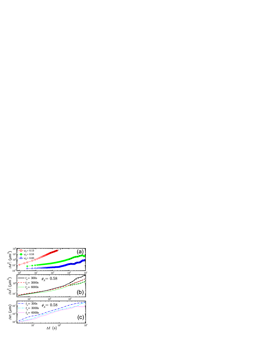
Figure 1:

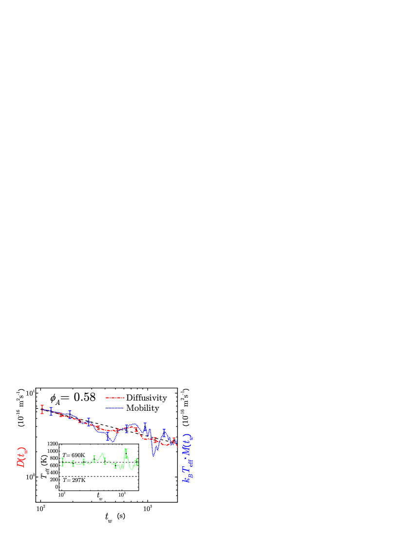
Figure 2:

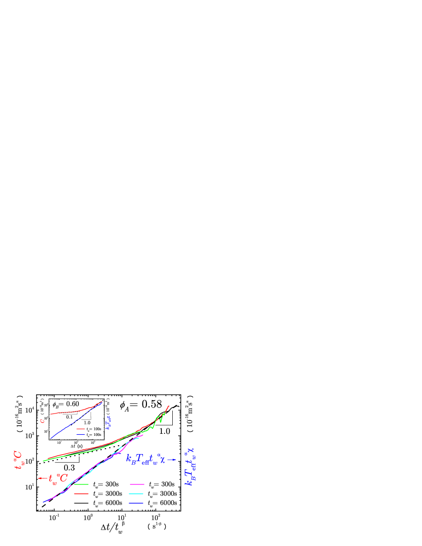
Figure 3:

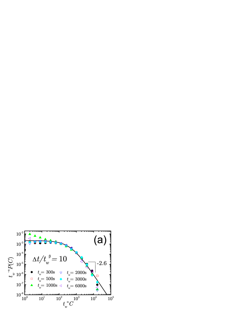
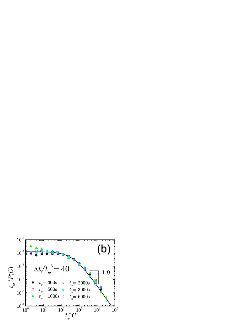
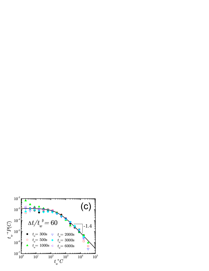
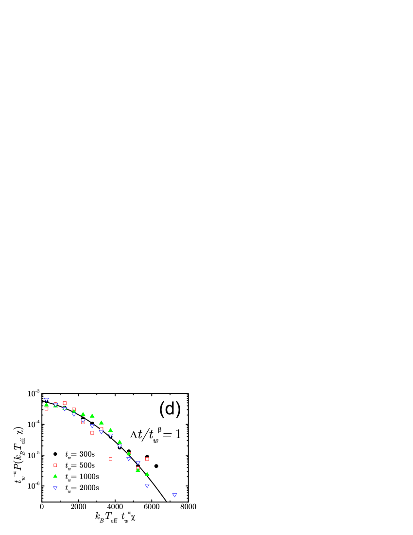
Figure 4:

SUPPLEMENTARY MATERIALS

Appendix A Details of the experimental set up

The experimental set up is shown in Fig. 5a and Fig. 5b. We use a Zeiss microscope with a 50$\times$ objective of numerical aperture 0.5 and a working distance of 5mm. We work with a field of view $194\mu m\times 155\mu m$ by using a digital camera with the resolution of 1288 pixels $\times$ 1032 pixels. We locate the center of each bead position with sub-pixel accuracy, by using image analysis. For the condensed samples A and B, we use the low frame rate $1/3$ frame/sec, while for the dilute sample C, we record the images at $1$ frame/sec. The long working distance of the objective is necessary to allow the pole of the magnet to reach a position near the sample. An example of the images of the tracers obtained in sample A is shown in Fig. 5a where we can see the black magnetic tracers embedded in the background of nearly transparent PMMA particles. An example of the trajectory in the x-y plane of a tracer diffusing without magnetic field is shown in Fig. 5d. We note that this particular tracer moves away from two cages in a time of the order of $4$ hours.

The magnetic field is produced by one coil made of 1200 turns of copper wire. We arrange the pole of the coil perpendicular to the vertical optical axis, and generate a field with no vertical component. Thus, the tracers move in the x-y plane with a slight vertical motion which is generated by a density mismatch between the tracers and the background PMMA particles. This vertical motion is very small at the high volume fraction of interest here, and therefore we calculate all the observables in the x-y plane.

The magnetic force is calibrated for a given coil current by replacing the suspension with a mixture of $50:50$ water-glycerol solution with a few magnetic tracers. The distance between the top of the magnetic pole and the vertical optical axis is always fixed, which means that the magnetic force at the local plane depends only on the coil current. At a given current, we determine the velocity of the magnetic tracers at the focal point and calculate the magnetic force from Stokes’s law, $F=6\pi\eta a_{m}v$, where $\eta$ is the viscosity of the water-glycerol solution, $a_{m}$ is the tracer radius, and $v$ is the observed velocity of the tracer. The uncertainty in the obtained force comes from: (a) the uncertainty in the coil current which is $1\%$, (b) the beads, which are not completely monodisperse in their magnetic properties, causes a $10\%$ uncertainty Weeks_force , and (c) the magnetic field is slowly decaying in the field of view, causing a $4\%$ uncertainty.

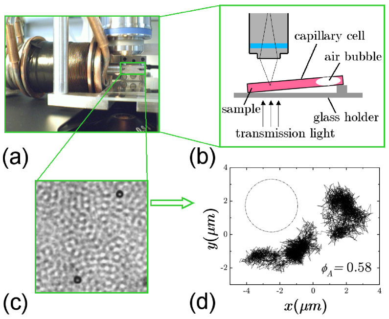
Figure 5: (a) Picture of the experimental setup. (b) Schematic illustration of the setup. (c) Detail of an image of tracer in sample A. (d) Trajectory of a tracer in sample A showing the cage dynamics over 4 hours. The circle represents the size of the tracer particle, $3.2\mu m$.

Appendix B Sample Preparation at $t_{w}=0$

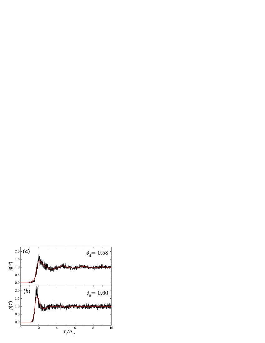
Figure 6: Pair-distribution functions of (a) sample A and (b) sample B.

It is important to correctly determine the initial time of each measurement to reproduce the subsequent particle dynamics. We initialize the system by stirring the sample for two hours with an air bubble inside the sample (see Fig. 5b) to homogenize the whole system and break up any pre-existing crystalline regions. Then we place the sample on the magnetic stage and take images to obtain the trajectories of the tracers that appear in the field of view. The initial times $t=t_{w}=0$ are defined at the end of the stirring. After measuring all the tracers appearing in the field of view, a new stirring is applied, the waiting time is reset to zero, and the measurements are repeated for a new set of tracers. We have analyzed the pair-distribution function, $g(r)$, and two-time intensity autocorrelation function, $g_{2}(t_{w},t_{w}+\Delta t)$, in order to test our rejuvenation technique.

First, Fig. 6 plots the pair-distribution functions of sample A and sample B right after the stirring procedure. We calculate the pair-distribution functions by reconstructing the packings from 3D confocal microscopy images of size $60\mu m{\times}60\mu m{\times}15\mu m$. We find that the samples do not show obvious crystallized region by directly looking either at the pair-distribution function or the images taken from confocal microscopy. For these measurements we use a Leica confocal microscope. The PMMA particles are fluorescently dyed so that they are ready to be observed by confocal microscopy. We load the samples sealed in a glass cell on the confocal microscope stage and use a Leica HCX PL APO 63x, 1.40 numerical aperture, oil immersion lens for 3D particle visualization in order to calculate the volume fraction and the pair-distribution function.

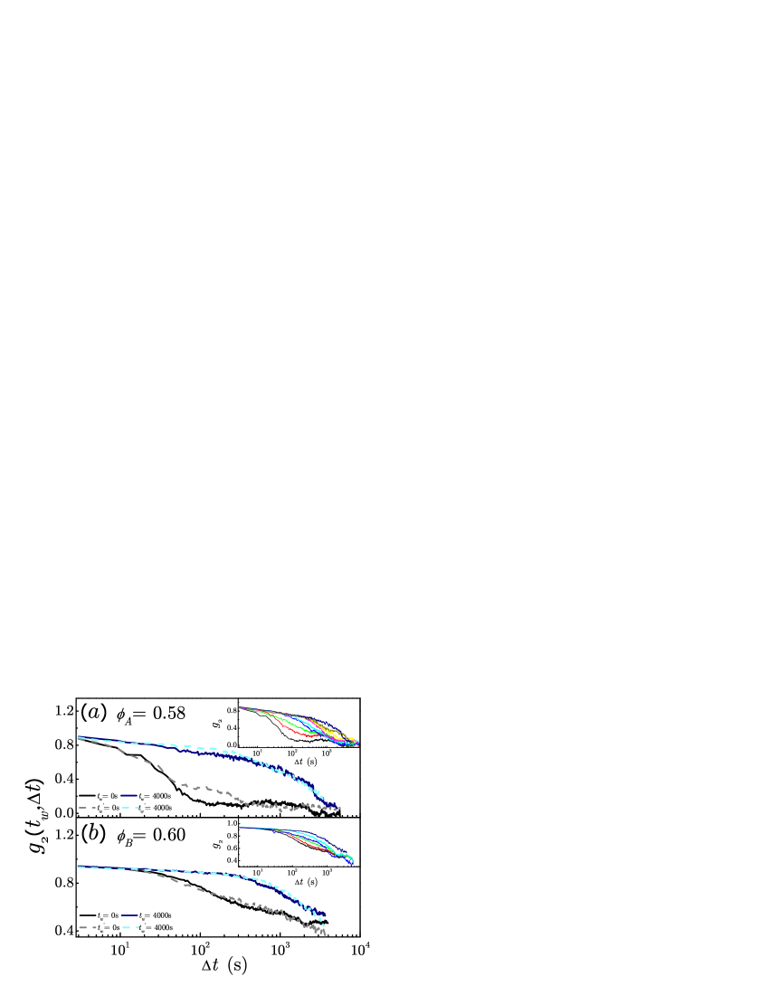
Figure 7: Two-time intensity autocorrelation function, $g_{2}(t_{w}+\Delta t,t_{w})$, of (a) sample A and (b) sample B. The solid black and navy curves correspond to $t_{w}=0$s and $t_{w}=4000$s, respectively. The dash gray and light blue curves correspond to the measurements after the second stirring with ${t_{w}}^{{}^{\prime}}=0$s and ${t_{w}}^{{}^{\prime}}=4000$s, respectively. The fact that the curves at $t_{w}=0$s and ${t_{w}}^{{}^{\prime}}=0$s coincide indicates that sample has been fully rejuvenated to its initial state. The inset is the same plot as the main figure for different $t_{w}$ ranging from 0s (solid black) to 4000s (solid navy).

Second, we analyze $g_{2}(t_{w}+\Delta t,t_{w})$ and show that the sample has been rejuvenated by the stirring process. We plot $g_{2}(t_{w}+\Delta t,t_{w})$ for 3 situations: (a) after the first stirring process ($t_{w}=0$), (b) after the sample has aged for a long time ($t_{w}=4000s$), (c) we then apply the stirring again and immediately plot the autocorrelation function for the new initial time (${t_{w}}^{{}^{\prime}}=0$). The plot show the lack of correlation for the two individual measurements $t_{w}=0$ and ${t_{w}}^{{}^{\prime}}=0$, thus demonstrating that the sample has been rejuvenated. Technically, we record the temporal image sequence of sample A and sample B, and study the aging by calculating two images’ correlation defined as:

$$g_{2}(t_{w},t_{w}+\Delta t)=\frac{\langle I(t_{w})I(t_{w}+\Delta t)\rangle}{\langle I(t_{w})^{2}\rangle},$$ (8)

where $I$ is the average gray-scale intensity of a small box (20 pixels $\times$ 20 pixels, PMMA particles’ diameter is roughly equal to 20 pixels), and $I(t_{w})$ and $I(t)$ come from the images at different times $t_{w}$ and $t$, respectively. We cut one image (1288 pixels $\times$ 1032 pixels) into many boxes, and calculate the correlation of two boxes located at the same position in the two images. The average $\langle...\rangle$ is taken over all the boxes in one image. Fig. 7 plots the correlation function, $g_{2}(t_{w},t_{w}+\Delta t)$, of sample A and sample B, which shows aging behavior (see the inset). Fig. 7 shows how $g_{2}(t_{w},t_{w}+\Delta t)$ calculated after two stirring processes at $t_{w}=0$ and ${t_{w}}^{{}^{\prime}}=0$ coincide, indicating that the sample can be fully rejuvenated to its initial state by our stirring technique.

Appendix C Data analysis

The average $\langle\cdot\cdot\cdot\rangle$ used to calculate the MSD $\langle\Delta x^{2}(t,t_{w})\rangle$ and the mean displacement $\langle\Delta x(t,t_{w})\rangle$ denotes an ensemble average over the tracers and over the initial time $t_{0}$ which is varied over a small time interval centered at $t_{w}$. We choose a small coarse-grained time interval compared to $t_{w}$, so that we can ignore the aging effect in such short time. We then regard all the trajectories in this interval region as having the same waiting time $t_{w}$. In practice, at a given $t_{w}$ and a given $\Delta t=t-t_{w}=t_{1}-t_{0}$, $(t>t_{w},t_{1}>t_{0})$, we use the common method (window_average , pages 118-122) of opening a small time window $[t_{w}-t_{r},t_{w}+t_{r}]$ and perform an average over all the $\Delta t$ with $t_{0}\in[t_{w}-t_{r},t_{w}+t_{r}]$ and $t_{1}\in[t_{w}-t_{r},t_{max}]$ in order to measure the transport coefficients. We note that $t_{r}<t_{w}$ and that $t_{max}$ is the maximum time of our measurements. The diffusion and mobility constants are then obtained by averaging not only over the tracers but also over the initial time $t_{0}$. This common technique allows us to obtain an estimation of the diffusion constant and mobility constant by using 82 tracers and 75 tracers respectively for this particular system. We check that by reducing the region size $t_{r}$ we obtain the same behavior of $D(t_{w})$ and $M(t_{w})$, so that the transport coefficients are independent of the averaging technique.

We collect all the tracers’ trajectories from several measurements since our system is well reproducible as described in Appendix A. In each measurement, we consider tracers that are separated by at least 10 particle diameters from the sample boundary and from each other. This guarantees that the tracer-tracer magnetic interaction can be ignored.

Appendix D $\Delta t$-linear regime

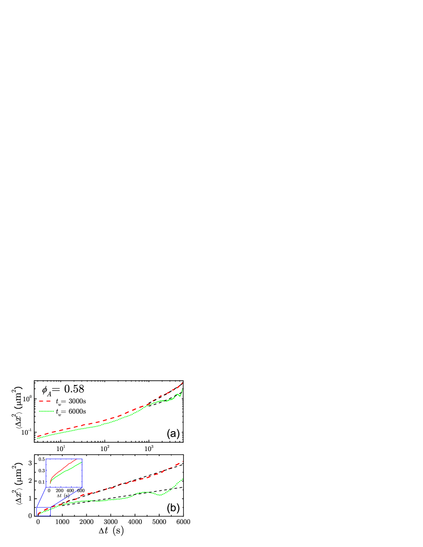
Figure 8: Mean square displacement of tracers as a function of $\Delta t$ for the sample A at $t_{w}=3000$s and $t_{w}=6000$s in (a) log-log plot and (b) linear-linear plot. The dashed lines are linear fittings of the $\Delta t$-linear regime.

In this appendix we address the issue of the proper determination of the long $\Delta t$-linear regime in the MSD where the diffusivity is calculated. The crossover from the cage dynamics regime to the long time diffusive regime seems to be very gradual in Fig. 1b (see for instance the case of $t_{w}=6000$s). We notice that due to the existence of the plateau in the MSD, the fitting to the long $\Delta t$-linear regime is of the form $\langle\Delta x^{2}\rangle\sim A(t_{w})+2D(t_{w})\Delta t$, where $A(t_{w})$ is a constant dependent only on $t_{w}$ and $D(t_{w})$ is the diffusion constant. Thus, in the log-log plot of Fig. 1, such a linear relation would not be a complete straight line. [note that the logarithmic plot is necessary to observe the different time scales in the experiment, and the fitting constant $A(t_{w})$ is the y-intercept of the fitting of the long $\Delta t$-linear regime, for which there is no particular physical meaning].

In order to address the issue of the existence of the long-time linear regime we compare a log-log plot of the MSD with a linear-linear plot of the same quantity for the sample A in Fig. 8a and Fig. 8b, respectively. We check our results for $t_{w}=3000$s and $t_{w}=6000$s.

First we note that the log-log plot of Fig. 8a naturally emphasizes the short time scales of the cage dynamics. Thus, a linear fitting function plus a constant, $\langle\Delta x^{2}\rangle=A(t_{w})+2D(t_{w})\Delta t$ would be represented as a smoothly varying curve for long $\Delta t$ in such a log-log plot, giving the impression that the long-time linear regime is not well-defined. In order to determine more clearly the large time regime we have plotted the MSD in a linear-linear plot in Fig. 8b. The $\Delta t$-linear regime and the fitting region can be more clearly seen from the linear-linear plot. The smaller $t_{w}$ are also plotted in the figure ($t_{w}=3000$s). As discussed above the linear-linear plot shows more clearly the existence of the linear regime while the log-log plot shows the existence of the cage dynamics regime.

We also note that the fast motion inside the cage is determined by the viscosity of the surrounding fluid, and not by the macroscopic viscosity which determines the $T_{\texttt{eff}}$ at long times. Indeed, the motion inside the cage is supposed to be equilibrated at room temperature and satisfies the regular FDT according to previous studies, for instance see simulations of Lennard-Jones liquids Barrat_Kob . The time scales for this microscopic viscosity to dominate is of the order of $10^{-2}$s, as obtained in light scattering experiments of colloidal glasses Megen_prl . These time scales are too fast to be studied with our visualization schemes. Our measurements start at $\Delta t\sim 1$s and go on up to $10^{4}$s. In this long time regime the microscopic viscosity does not dominate the dynamics and indeed we find the $T_{\texttt{eff}}$ is dominated by the macroscopic viscosity given by the particles.

From Stokes-Einstein relation, $F=6\pi a_{m}\eta\upsilon$, with $F\sim 10^{-14}N$, $\eta\sim 10^{-3}N.s.{m}^{-2}$ the viscosity of the decalin-bromide solution, $a_{m}\sim 3\mu m$ the tracer’s diameter and $\Delta t\sim 10^{-2}$s, we find $\Delta x\sim 0.002\mu m$. At this length scale the particle experience the viscosity of the surrounding liquid alone. Since we measure much larger displacements, we conclude that the tracers are experiencing the macroscopic viscosity and the effective temperature is therefore well defined.

Therefore, we believe that we have achieved the necessary separation of length scales which allows us to define a $T_{\texttt{eff}}$. The small displacements observed in the response function are due to the fact that the magnetic forces ought to be small enough to achieve the linear response regime. The small displacements obtained in our measurements are consistent with previous confocal microscopy studies of colloidal suspensions near the glass transition Weeks_prl , which found motions of the order of $1/10$ of the particle diameter.

Appendix E Study of samples C

Figure 9 shows the parametric plot of correlation function $C$ versus integrated response function $k_{B}\chi$ for the dilute sample C, $\phi_{C}=0.13$. We find $M=3.28\times 10^{7}$ms^-1N^-1 and $D=1.46\times 10^{-13}$m²s^-1, corroborating that this sample is equilibrated at the bath temperature $T=(323\pm 30)$K within the uncertainty of the experiment.

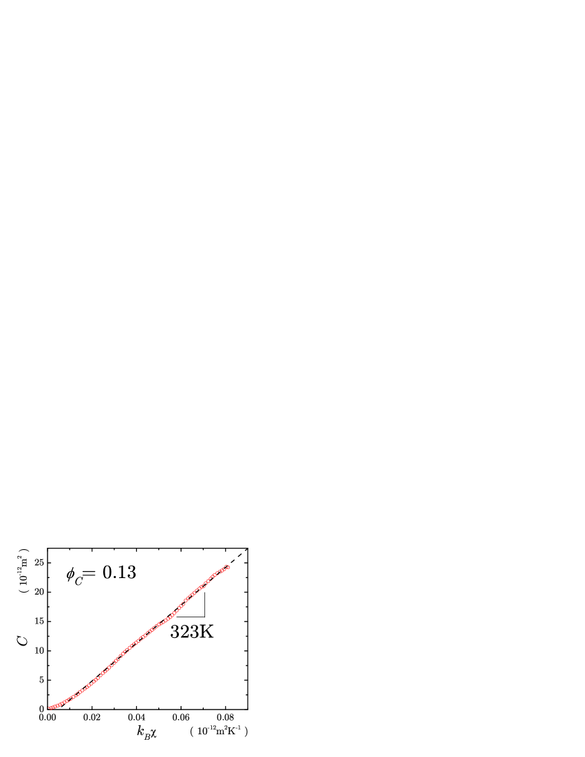
Figure 9: Parametric plot of correlation versus integrated response function for dilute sample C. The fitting line shows that the temperature of sample C, $T=(323\pm 30)$K, is close to the bath temperature ($T_{\rm bath}=297$K) in our experiment.

Appendix F Linear response regime

It is important to test for a well-defined linear response regime for small enough external forces where the mobility becomes independent of the force. Indeed, previous work Weeks_force did not find a linear regime, but instead there is a threshold force below which the particles are trapped even under the influence of the external force. On the contrary, here we find that if the observable time is larger than the cage life time, particles are always able to explore the structural relaxation leading to cage rearrangements, either in the presence or in the absence of the external force and therefore the linear response regime ensues. This is because the present experiments focus on larger time scales than previous work.

In order to find the linear response regime, we apply different forces for samples A and B. The results are shown in Fig. 10a and Fig. 10b. The collapsing of the results onto a single curve of $\langle\Delta x\rangle/F$ suggest a linear response for lower forces. The insets show the relationship between the velocity, $V_{x}=\langle\Delta x\rangle/\Delta t$, of the tracers along the force direction and the force $F$, which indicates that the external force cannot be larger than $4\times 10^{-14}$N and $6\times 10^{-14}$N to keep the linear response for samples A and B, respectively. It then confirms that the force $F=1.7\times 10^{-14}$N used in our studies is in the linear response regime.

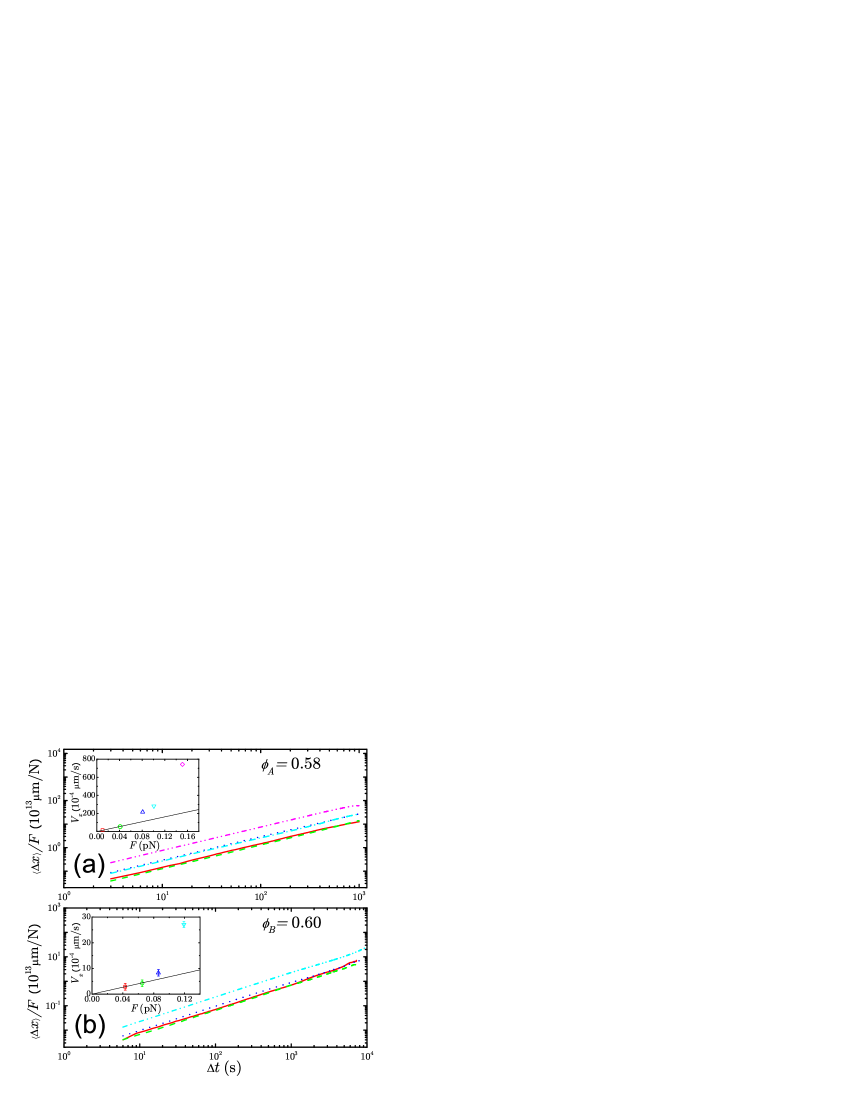
Figure 10: The response functions for (a) sample A and (b) sample B. The insets are plots of the velocity of magnetic beads as a function of the force, $V_{x}$ versus $F$. The straight line indicates the linear response regime. The velocity error is due to the accuracy to locate the bead positions, smaller than the symbol size in the inset of (a).

It is important to investigate the age-dependence of the linear response. As we addressed in the original manuscript, many measurements have to be taken to reveal the aging behavior for one value of the external force. Therefore to measure the aging effect in Fig. 1c, we measured over 75 trajectories to achieve a statistically reliable average. In order to find the region of forces in the linear response regime, many experiments have to be run at different forces. Thus, for the determination of the linear response we are obliged to use a smaller number of tracers (roughly 10). In this case, in order to improve the statistical average, we average over the waiting time $t_{w}$ and obtain a single velocity $V_{x}$ for each force, as shown in Fig. 10. (The aging dependence is ignored, and the response functions as shown in Fig. 10 are calculated by regular time-translation-invariance methods). This average is only applied to find the value of the external force in the linear response regime. Once this force is identified, then we perform the full aging analysis by measuring a larger amount of tracers.

Appendix G Sedimentation of magnetic tracers

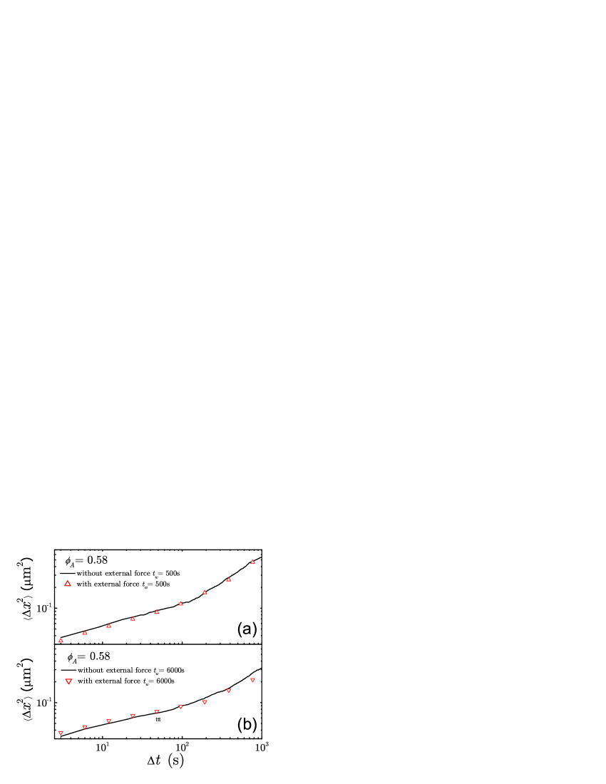
Figure 11: MSD for the sample A at (a) $t_{w}=500$s and (b) $t_{w}=6000$s analyzed from the data without magnetic force and with magnetic force, respectively.

The density of the magnetic tracers is very close to the background PMMA particles. Since the sedimentation is proportional to the mismatch between the density of the tracers and the surrounding liquid (which is the same as the PMMA density), then we expect that the effect of sedimentation would be small.

In principle, this effect is negligible in the more dense sample B since the tracers remain in the x-y plane for few hours without any noticeable sedimentation effect. In the case of the less concentrated sample A, sedimentation of tracers can be seen after one hour of observation. Since we measure up to $t_{w}=6000$s, it is important to check the effect of sedimentation on the diffusion of particles for this sample.

Unfortunately, we cannot test directly the effect of this sedimentation, since we cannot match the density of the tracers with that of the fluid and PMMA particles (the tracers are magnetic and therefore slightly heavier than the PMMA particles by construction). However we can indirectly test the main issue at hand: What is the effect of an external driving constant force of the order of gravity ($\sim$pN) on the tracer diffusion?

To this end we apply a magnetic external force of the same value as the sedimentation force and measure the resulting effect on the diffusion constant for sample A. We found that the effect of the external force on diffusion is negligible as long as the force is small enough ($\sim$pN). Figure 11 plots the MSD for the sample A at (a) $t_{w}=500$s and (b) $t_{w}=6000$s. We obtain the MSD analyzing the trajectories of tracers without magnetic force and with magnetic force (in this case, we properly subtract the average value of the displacements). The figure indicates that the diffusion is the same with or without the external force, thus confirming its negligible effect for this case.

Appendix H Determination of the aging exponents

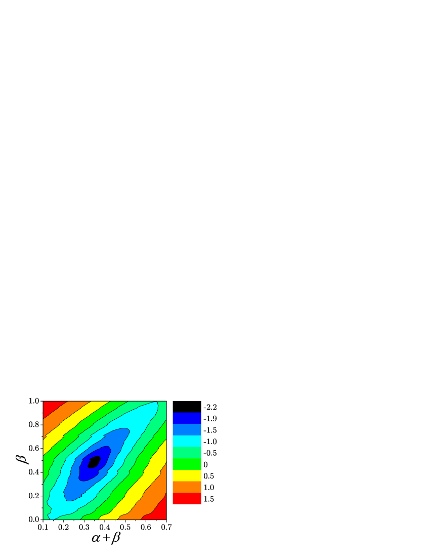
Figure 12: Log plot of standard deviation, $\ln\sigma^{2}$, which quantifies the collapsing of $t_{w}^{\alpha}C(t_{w},t_{w}+\Delta t)$ for all the data of sample A (in color scale or gray scale). The minimum of $\sigma^{2}$ (black basin) gives the best aging exponents at $\alpha+\beta=0.34\pm 0.05$, $\beta=0.48\pm 0.05$.

As described in the main manuscript, all the MSD for different aging times $t_{w}$ collapse onto a master curve when plotted as $t_{w}^{\alpha}C(t_{w},t_{w}+\Delta t)$ versus $\Delta t/{t_{w}}^{\beta}$. In order to search for the best value of the aging exponents $\alpha$ and $\beta$ that give the correct data collapse, we calculate the standard deviation of all the curves as defined below:

$$\begin{split}&\sigma^{2}=\sum_{\ln(\Delta t/t_{w}^{\beta})}\sum_{\ln(t_{w})}\\ &[\ln(t_{w}^{\alpha}C(t_{w},\Delta t/t_{w}^{\beta}))-\frac{1}{N}\sum_{\ln(t_{w})}\ln(t_{w}^{\alpha}C(t_{w},\Delta t/t_{w}^{\beta}))]^{2}.\end{split}$$ (9)

We search a wide range of $\alpha$ and $\beta$ to minimize $\sigma^{2}$. The result is plotted in Fig. 12 showing that the best data collapsing with $\sigma^{2}=0.1$ can be achieved at $\alpha+\beta=0.34\pm 0.05$ and $\beta=0.48\pm 0.05$ as reported in the main text.

Spin-glass models predict a general scaling form $C_{\rm ag}(t,t_{w})=C_{\rm ag}(h(t)/h(t_{w}))$, where $h(t)$ is a generic monotonic function Cugliandolo . In particular, a familiar form is $h(t)\sim t^{\mu}$ where $\mu$ is a power law exponent giving rise to the cases of simple aging, $\mu=1$, super aging, $\mu>1$, and sub-aging, $\mu<1$. Assuming the above form, the linear behavior $C_{\rm ag}(t_{w}+\Delta t,t_{w})\sim\Delta t$ for larger $\Delta t$ requires $\mu=1$. This is just a special case of our scaling ansatz Eq. (5a) with $\beta=1$. As we show in Fig. 12, our data cannot be collapsed for this parameter.

Appendix I Scaling behavior of local fluctuations

The local correlation function $C$ and local integrated response function $\chi$ studied in the manuscript are calculated from each individual tracer trajectory. In a condensed colloidal sample, the tracer trajectories are always confined at a local position. Therefore, the correlation $C$ and response $\chi$ for an individual particle can be regarded as the coarse-grained local fluctuations of the observables as investigated in Castillo .

Furthermore, in order to improve the statistics of our results, the PDF $P(C)$ is calculated not only for all the tracers, but also over a time interval much smaller than the age of the system. In practice, we calculate the $i-$th tracer’s local correlation function as $C_{i}(t_{w}+\Delta t,t_{w})$. At a given $\Delta t$, we open a small time window $[\Delta t-t_{s},\Delta t+t_{s}]$ ($t_{s}\ll\Delta t$) and count all the $C_{i}(t_{w}+\Delta t_{j},t_{w})$ with $\Delta t_{j}\in[\Delta t-t_{s},\Delta t+t_{s}]$ into the statistics of $P(C)$. The calculated $P(C)$ is a mixture of the local and the temporal fluctuations of the observables. Similar technique is performed to calculate $P(\chi)$.

Below we derive the scaling law for the PDF of the local correlation function, Let us first recall the scaling behavior of the global correlation function in Eq. (5),

$$t_{w}^{\alpha}\overline{C(t_{w}+\Delta t,t_{w})}=f_{D}({\Delta t}/{{t_{w}}^{\beta}}),$$ (10)

where we add a bar to $\overline{C}$ to distinguish the global correlations from the local $C$. The average is taken over all the tracer particles. We can rewrite the global correlation function as the integration of the PDF $P(C)$ as:

$$\overline{C}=\int P(C)CdC.$$ (11)

Furthermore, we obtain the relation of $f_{D}$ and $P(C)$ by substituting Eq. (11) into Eq. (10):

$$f_{D}({\Delta t}/{{t_{w}}^{\beta}})=t_{w}^{\alpha}\overline{C}=\int t_{w}^{-\alpha}P(C)(t_{w}^{\alpha}C)d(t_{w}^{\alpha}C).$$ (12)

For a given ${\Delta t}/{{t_{w}}^{\beta}}$, $f_{D}$ is equal to a constant, and Eq. (12) requires that $t_{w}^{-\alpha}P(C)$ should only depend on $t_{w}^{\alpha}C$. In other words, $t_{w}^{-\alpha}P(C)$ is a function of ${\Delta t}/{{t_{w}}^{\beta}}$ and $t_{w}^{\alpha}C$. Then we define $F_{D}$ as:

$$F_{D}(t_{w}^{\alpha}C,\Delta t/t_{w}^{\beta})=t_{w}^{-\alpha}P(C).$$ (13)

A similar formula can be obtained for $P(\chi)$. Eventually, we obtain the scaling ansatz of $P(C)$ and $P(\chi)$ shown in Fig. 4:

$$P(C) =t_{w}^{\alpha}F_{D}(t_{w}^{\alpha}C,\Delta t/t_{w}^{\beta}),$$ (14a)

$$P(\chi) =t_{w}^{\alpha}F_{M}(t_{w}^{\alpha}\chi,\Delta t/t_{w}^{\beta}),$$ (14b)

where the universal functions $F_{D}(x,y)$ and $F_{M}(x,y)$ satisfy

$$\int F_{D}(x,y)dx=f_{D}(y),$$ (15a)

$$\int F_{M}(x,y)dx=f_{M}(y).$$ (15b)

Appendix J Study of the PDF of the autocorrelation function

The PDF of the autocorrelation function follows a modified power law $t_{w}^{-\alpha}P(C)\propto(t_{w}^{\alpha}C+C_{0})^{-\lambda}$, as we see in Figs. 4a, 4b and 4c. From Eq. (12), we have

$$\begin{split}t_{w}^{\alpha}\overline{C}&=\int_{0}^{C_{cut}}t_{w}^{-\alpha}P(C)(t_{w}^{\alpha}C)d(t_{w}^{\alpha}C)\\ &=\frac{\int_{0}^{C_{cut}}(x+C_{0})^{-\lambda}xdx}{\int_{0}^{C_{cut}}(x+C_{0})^{-\lambda}dx}.\end{split}$$ (16)

The cutoff $C_{cut}$ ($C_{cut}\gg C_{0}$) is introduced to make the integral converge and we always take $\lambda\geq 1$, then

$$t_{w}^{\alpha}\overline{C}=\frac{C_{0}}{\lambda-2}[1-(\lambda-1)(\frac{C_{cut}}{C_{0}}+1)^{2-\lambda}].$$ (17)

For $\lambda>2$, the last term in Eq. (17) is negligible and $t_{w}^{\alpha}\overline{C}\approx C_{0}/(\lambda-2)$ mainly depends on the short-time parameter $C_{0}$. For $\lambda<2$, we have $t_{w}^{\alpha}\overline{C}\approx\frac{\lambda-1}{2-\lambda}C_{0}(\frac{C_{cut}}{C_{0}})^{2-\lambda}$ and the long-time parameter $C_{cut}$ dominates.

Following the previous discussion of $P(C)$, we define the $i$-th tracer’s local correlation function as:

$$C_{i}(t_{w}+\Delta t,t_{w})=\langle\Delta x(t_{w}+\Delta t,t_{w})^{2}\rangle_{i}/2,$$ (18)

where the average $\langle...\rangle_{i}$ is calculated for only the $i$-th tracer’s trajectory by opening a small time window $[\Delta t-t_{s},\Delta t+t_{s}]$ ($t_{s}\ll\Delta t$) at a given $\Delta t$, and counting all the $C_{i}(t_{w}+\Delta t_{j},t_{w})$ with $\Delta t_{j}\in[\Delta t-t_{s},\Delta t+t_{s}]$ into the statistics of $P(C)$. We should note that if there is no average $\langle...\rangle_{i}$, $P(C)$ can be reduced to a simple form:

$$P(C)=P(\langle\Delta x^{2}\rangle_{i}/2)\xrightarrow{\langle...\rangle_{i}\rightarrow 0}P(\Delta x^{2}/2).$$ (19)

This form can be further reduced since

$$P(\Delta x^{2}/2)d(\Delta x^{2}/2)=P(\Delta x)dx,$$ (20)

therefore at the limit of the average $\langle...\rangle_{i}\rightarrow 0$,

$$P(C)=P(\langle\Delta x^{2}\rangle_{i}/2)\xrightarrow{\langle...\rangle_{i}\rightarrow 0}P(\Delta x^{2}/2)=P(\Delta x)/{\Delta x}.$$ (21)

Therefore our $P(C)$ is relate to the probability $P(\Delta x)$ usually studied in previous works Weeks_sci . We find that $P(\Delta x)$ can be approximately fitted by a broad tail power law behavior for large $\Delta x$, consistent with equation 21. However the data of $P(\Delta x)$ can be better fitted by stretch exponential rather than power law, which is consistent with previous works Weeks_sci . On the contrary, $P(\langle\Delta x^{2}\rangle_{i}/2)$ can not be fitted by stretch exponential. Thus we believe that the power law fit is more proper to describe our result of $P(C)$. The difference with other studies might be due to the fact that our samples are glassy while others work in the supercooled regime.

References

- (1) Pusey, P. N. & van Megen, W. Phase behavior of concentrated suspensions of nearly hard colloidal spheres. Nature 320, 340-342 (1986).
- (2) Cugliandolo, L. F. in Slow Relaxations and Nonequilibrium Dynamics in Condensed Matter, Barrat, J. -L. et al. (eds.) (Springer-Verlag, 2002).
- (3) Struik, L. C. E. in Physical Ageing in Amorphous Polymer and other Materials, (Elsevier, Houston, 1978).
- (4) Cugliandolo, L. F. & Kurchan, J. Analytical solution of the off-equilibrium dynamics of a long-range spin-glass model Phys. Rev. Lett. 71, 173-176 (1993).
- (5) Bouchaud, J. -P., Cugliandolo, L. F., Kurchan, J., & Mézard, M. in Spin-Glasses and Random Fields, (World Scientific, 1998).
- (6) Kirkpatrick, T. R. & Thirumalai, D. p-spin-interaction spin-glass models: connections with the structural glass problem. Phys. Rev. B 36, 5388-5397 (1987).
- (7) Bouchaud, J. -P., Cugliandolo, L. F., Kurchan, J. & Mézard, M. Mode-coupling approximations, glass theory and disordered systems. Physica A 226, 243-273 (1996).
- (8) Edwards, S. F. The role of entropy in the specification of a powder, in Granular matter: an interdisciplinary approach (ed. Mehta, A.) 121-140 (Springer-Verlag, New York, 1994).
- (9) Ono, I. K., O’Hern, C. S., Durian, D. J., Langer, S. A., Liu, A. J. & Nagel, S. R. Effective temperatures of a driven system near jamming. Phys. Rev. Lett. 89, 095703 (2002).
- (10) Makse, H. A. & Kurchan, J. Testing the thermodynamic approach to granular matter with a numerical model of a decisive experiment. Nature 415, 614-617 (2002)
- (11) D’Anna, G. & Gremaud, G. The jamming route to the glass state in weakly perturbed granular media. Nature 413, 407-409 (2003).
- (12) Song, C., Wang, P. & Makse, H. A. Experimental measurement of an effective temperature for jammed granular materials. Proc. Nat. Acad. Sci. 102, 2299-2304 (2005).
- (13) Stillinger, F. H. A topographic view of supercooled liquids and glass formation. Science 267, 1935-1939 (1995).
- (14) Kob, W., Sciortino, F., & Tartaglia, P. Aging as dynamics in configurations space. Europhys. Lett. 49, 590-596 (2000).
- (15) Israeloff, N. E. & Grigera, T. S. Low-frequency dielectric fluctuations near the glass transition. Europhys. Lett 43, 308-313 (1998).
- (16) Bellon, L., Ciliberto, S. & Laroche, C. Violation of the fluctuation-dissipation relation during the formation of a colloidal glass. Europhys. Lett. 53, 511-517 (2001).
- (17) Hérisson, D. & Ocio, M. Fluctuation-dissipation ratio of a spin glass in the aging regime. Phys. Rev. Lett. 88, 257202 (2002).
- (18) Buisson, L., Ciliberto, S. & Garcimartín, A. Intermittent origin of the large violations of the fluctuation-dissipation relations in an aging polymer glass. Europhys. Lett. 63, 603-609 (2003).
- (19) Abou, B. & Gallet, F. Probing a nonequilibrium Einstein relation in an aging colloidal glass. Phys. Rev. Lett. 93, 160603 (2004).
- (20) Parisi, G. Off-equilibrium fluctuation-dissipation relation in fragile glasses. Phys. Rev. Lett. 79, 3660-3663 (1997).
- (21) Barrat, J. -L. & Kob, W. Fluctuation-dissipation ratio in an aging Lennard-Jones glass. Europhys. Lett. 46, 637-642 (1999).
- (22) Berthier, L. & Barrat, J. -L. Nonequilibrium dynamics and fluctuation-dissipation in a sheared fluid. J. Chem. Phys. 116, 6228-6242 (2002).
- (23) Kegel, W. K. & van Blaaderen, A. Direct observation of dynamical heterogeneities in colloidal hard-sphere suspensions. Science 287, 290-293 (2000).
- (24) Weeks, E. R., Crocker, J. C., Levitt, A. C., Schofield, A. & Weitz, D. A. Three-dimensional direct imaging of structural relaxation near the colloidal glass transition. Science 287, 627-631 (2000).
- (25) Megen, W. van, Underwood, S. M. Glass transition in colloidal hard spheres: Mode-coupling theory analysis. Phys. Rev. Lett. 70, 2766-2769 (1993).
- (26) Courtland, R. E., Weeks, E. R. Direct visualization of ageing in colloidal glasses. J. Phys.: Condens. Matter 15, S359-S365 (2003).
- (27) Henkel, M., Pleimling, M., Godrèche, G. & Luck, J. -M. Aging, phase ordering, and conformal invariance. Phys. Rev. Lett. 87, 265701 (2001).
- (28) Cugliandolo, L. F., Kurchan, J., & Doussal, P. L. Large Time Out-of-Equilibrium Dynamics of a Manifold in a Random Potential. Phys. Rev. Lett. 76, 2390-2393 (1996).
- (29) Bustingorry, S., Cugliandolo, L. F., & Dominguez, D. Out-of-Equilibrium Dynamics of the Vortex Glass in Superconductors. Phys. Rev. Lett. 96, 027001 (2006).
- (30) Kob, W., Donati, C., Plimpton, S. J., Poole, P. H., & Glotzer, S. C. Dynamical heterogeneities in a supercooled Lennard-Jones liquid. Phys. Rev. Lett. 79, 2827-2830 (1997).
- (31) Castillo, H. E., Chamon, C., Cugliandolo, L. F. & Kennett, M. P. Heterogeneous aging in spin glasses. Phys. Rev. Lett. 88, 237201 (2002).
- (32) Amblard, F., Yurke, B., Pargellis, A. N. & Leibler, S. A magnetic manipulator for studying local rheology and micromechanical properties of biological systems. Rev. Sci. Instrum. 67, 818-827 (1996).
- (33) Habdas, P. et al. Forced motion of a probe particle near the colloidal glass transition. Europhys. Lett. 67, 477-483 (2004).
- (34) Rapaport, D. C. (1995) The Art of Molecular Dynamics Simulation, (Cambridge Univ. Press, Cambridge, U.K.).
- (35) Weeks, E. R., Weitz, D. A. Properties of Cage Rearrangements Observed near the Colloidal Glass Transition. Phys. Rev. Lett. 89, 095704 (2002)
Acknowledgements.
We wish to thank M. Shattuck for help in the design of the experiments and J. Brujić and S. Mistry for providing the colloidal particles and illuminating discussions. We acknowledge the financial support from DOE and NSF. Correspondance should be addressed to H. A. Makse.FIG. 1. Autocorrelation and response functions. (a) Mean square displacement of tracers as a function of for the three samples at s. The straight dash lines indicate estimates for the diffusivity . (b) Mean square displacement of tracers in sample A as a function of time , for various aging times . The dashed straight lines indicate the fitting regime to calculate the diffusivity . (c) Mean displacement of tracers under the magnetic force in sample A for various aging times .