Raman scattering for triangular lattices spin-$\frac{1}{2}$ Heisenberg antiferromagnets

Abstract

Motivated by various spin-1/2 compounds like Cs₂CuCl₄ or $\kappa$-(BEDT-TTF)₂Cu₂(CN)₃, we derive a Raman-scattering operator à la Shastry and Shraiman for various geometries. For T=0, the exact spectra is computed by Lanczos algorithm for finite-size clusters. We perform a systematic investigation as a function of $J_{2}/J_{1}$, the exchange constant ratio: ranging from $J_{2}=0$, the well known square-lattice case, to $J_{2}/J_{1}=1$ the isotropic triangular lattice. We discuss the polarization dependence of the spectra and show how it can be used to detect precursors of the instabilities of the ground state against quantum fluctuations.

1 Introduction

Highly frustrated magnetic systems are highly susceptible to quantum spin fluctuations and instabilities towards competing ground states. The triangular Heisenberg antiferromagnet with spin $S=1/2$ constitutes a paradigm of that class of systems. In that context, it is interesting that experimental investigations of the Cs₂CuCl₄ [1] and $\kappa$-(BEDT-TTF)₂Cu₂(CN)₃ [2] materials, which can be both described as a first approximation by a triangular lattice with spatially anisotropic exchange couplings, indicate exotic behaviors. Exotic behaviors include either the realization of a spin-liquid ground state or a magnetically ordered phase with a magnetic excitation dispersion strongly renormalized compared to the classical spin-wave. Indeed, recent numerical studies based on series expansion [3] have found that frustration manifests itself rather directly in the spin excitations of archetype models of two-dimensional frustrated spin systems. A softening of the magnon excitations in a broad region of the reciprocal ${\bm{q}}$ space is observed as a quantity, $f$, which parametrize the level of frustration, is increased. Since, within a semi-classical picture, the effect of frustration is to bring about the effect of competing ground states, it is expected that the spin excitations out of a semi-classical long-range ordered ground state are direct tell-tale indicators of the presence of frustrating interactions. In this paper we explore the possibility that frustration can also be investigated via the two-magnon density of states at zero wavevector measured by polarized inelastic magnetic Raman scattering.
The rest of this paper is organized as follows: in the first Section we present the derivation of the scattering operator, then we discuss its form for various polarizations. In the last part we present the associated Raman spectra obtained by exact-diagonalization of finite-size clusters.

2 Scattering operator

We first consider the Hubbard model on the anisotropic triangular lattice:

$${\mathcal{H}}={\mathcal{H}}_{K}+{\mathcal{H}}_{U}=\sum_{\langle i,j\rangle,\sigma}t_{ij}\left(c^{\dagger}_{i,\sigma}c_{j,\sigma}+h.c.\right)+U\sum_{i}n_{i,\uparrow}n_{i,\downarrow}$$ (1)

where $t_{ij}$ is the hopping from a site $i$ to a neighboring site $j$, $\sigma$ is the spin degree of freedom, and $c$ and $c^{\dagger}$ are the usual annihilation and creation operators. For the case considered here, there are two distinct hopping integrals, $t_{1}$ and $t_{2}$, along the corresponding directions shown in Fig. 1.

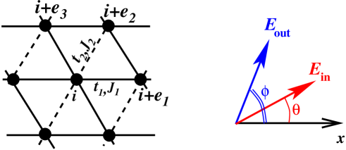
Figure 1: Geometry of the lattice and polarization vectors. Left: The dashed lines represent the coupling $J_{2}$, the thick lines are for the exchange coupling $J_{1}$. Right: Definition of the polarization vectors by two angles $\phi$ and $\theta$.

At half-filling and in the large-$U$ limit, the system is described (to second order in $t/U$) by an effective spatially anisotropic Heisenberg Hamiltonian:

$${\mathcal{H}}_{\rm eff}=\sum_{\langle i,j\rangle}J_{ij}{\bf S}_{i}\cdot{\bf S}_{j}$$ (2)

where the different exchange coupling along each direction is due to the difference in the hopping amplitude, i.e $J_{1}=4t^{2}_{1}/U$ , $J_{2}=4t^{2}_{2}/U$.
Raman scattering consists of an incoming photon (of energy $\omega_{i}$) scattered into an outgoing photon (of energy $\omega_{f}$), involving different manifold of electronic states having zero or one double-occupancy. These transitions depend on the polarizations (referred as E_in and ${\bf E}_{\rm out}$) of the incoming and outgoing photons. Following the early work of Fleury and Loudon [4] and Shastry and Shraiman [5], we derive an effective scattering spin Hamiltonian describing this problem. The $\alpha$-component of the electronic hopping current operator is:

$$j^{\alpha}({\bf q})=i\sum_{{\bf r},{\bm{\nu}}=\pm({\bf e_{1},e_{2},e_{3}})}\left(\frac{\partial\epsilon_{\bf k}}{\partial k^{\alpha}}\right)e^{i{\bf q}\cdot({\bf r}+\frac{{\bm{\nu}}}{2})}\left[c^{\dagger}_{\sigma}({\bf r}+{\bm{\nu}})c_{\sigma}({\bf r})-c^{\dagger}_{\sigma}({\bf r})c_{\sigma}({\bf r}+{\bm{\nu}})\right]$$ (3)

where ${\bf q}={\bf k}_{f}-{\bf k}_{i}$ is the momentum transfer, and $\epsilon_{\bf k}$ the band-energy. In what follows we take the most general set of polarization vectors, as shown in the right panel of Fig. 1:

$$\left\{\begin{array}[]{rcl}\cos\phi\ \hat{x}&+&\sin\phi\ \hat{y}\\ \cos\theta\ \hat{x}&+&\sin\theta\ \hat{y}\\ \end{array}\right.$$ (4)

The Raman scattering process involves an energy transfer $\Omega=\omega_{f}-\omega_{i}$, the momentum transfer being set to zero. Therefore, we restrict ourselves to the assumption ${\bf k}_{f}\approx{\bf k}_{i}\approx 0$, and we have:

$$\begin{array}[]{c}{\bf j}\cdot{\bf E}_{\rm in}=i\cos\phi\left[-t_{1}\left(c^{\dagger}_{r}c_{r+{\bf e}_{1}}-h.c\right)\right.\left.-\frac{t_{2}}{2}\left(c^{\dagger}_{r}c_{r+{\bf e}_{2}}-h.c\right)\right.\\ \left.+\frac{t_{1}}{2}\left(c^{\dagger}_{r}c_{r+{\bf e}_{3}}-h.c\right)\right]\\ -i\frac{\sqrt{3}}{2}\sin\phi\left[t_{2}\left(c^{\dagger}_{r}c_{r+{\bf e}_{2}}-h.c\right)+t_{1}\left(c^{\dagger}_{r}c_{r+{\bf e}_{3}}-h.c\right)\right]\\ \\ {\bf j}\cdot{\bf E}_{\rm out}=i\cos\theta\left[-t_{1}\left(c^{\dagger}_{r}c_{r+{\bf e}_{1}}-h.c\right)\right.\left.-\frac{t_{2}}{2}\left(c^{\dagger}_{r}c_{r+{\bf e}_{2}}-h.c\right)\right.\\ \left.+\frac{t_{1}}{2}\left(c^{\dagger}_{r}c_{r+{\bf e}_{3}}-h.c\right)\right]\\ -i\frac{\sqrt{3}}{2}\sin\theta\left[t_{2}\left(c^{\dagger}_{r}c_{r+{\bf e}_{2}}-h.c\right)+t_{1}\left(c^{\dagger}_{r}c_{r+{\bf e}_{3}}-h.c\right)\right]\\ \end{array}$$ (5)

The Raman scattering operator is given by the second order formula, $|i\rangle$ and $|f\rangle$ being respectively the initial and final state, $|\mu\rangle$ being an intermediate state:

$$\begin{array}[]{rcl}\langle f|M_{r}|i\rangle&=&\sum_{\mu}\left[\frac{\langle f|{\bf j}\cdot{\bf E}_{\rm out}|\mu\rangle\langle\mu|{\bf j}\cdot{\bf E}_{\rm in}|i\rangle}{\epsilon_{\mu}-\epsilon_{i}-\omega_{i}}\right.+\left.\frac{\langle f|{\bf j}\cdot{\bf E}_{\rm in}|\mu\rangle\langle\mu|{\bf j}\cdot{\bf E}_{\rm out}|i\rangle}{\epsilon_{\mu}-\epsilon_{i}+\omega_{f}}\right]\end{array}$$ (6)

Following the same algebra steps as in [5], and restricting $|i\rangle$ and $|f\rangle$ to the manifold of singly occupied states, and intermediate states $|\mu\rangle$ to the manifold of one double occupancy, we use the identity, $\frac{1}{4}-{\bf S}_{i}\cdot{\bf S}_{j}=\sum_{\sigma,\sigma^{\prime}}\frac{1}{2}c^{\dagger}_{i,\sigma}c_{j,\sigma}c^{\dagger}_{j,\sigma^{\prime}}c_{i,\sigma^{\prime}}$, and obtain the scattering operator in terms of spin operators. We note that within our approach the total scattering operator only contains terms of the form:

$${\mathcal{O}}_{\nu}\propto\frac{t_{\nu}^{2}}{U}{\bf S}_{i}\cdot{\bf S}_{i+{\bf e}_{\nu}}$$ (7)

From Eq. (6) we find that the scattering Hamiltonian prefactors which will be in front of Eq. (7) depend on the polarization vectors orientation. These prefactors are proportional to the exchange coupling $J$, therefore, in its general form, the total scattering operator will depend on both $J_{1}$ and $J_{2}$.

3 Polarizations

The two angles $\phi$ and $\theta$ with respect to the $x$-axis (see Fig. 1) define the polarizations involved in the scattering process. Therefore the scattering operator depends on a projector ${\mathcal{P}}_{\nu}(\theta,\phi)$ that defines the polarization set-up. The Raman operator takes the form:

$$\begin{array}[]{c}{\mathcal{H}}_{LF}(\theta,\phi)\propto\sum_{i}\left\{J_{1}{\bf S}_{i}\cdot{\bf S}_{i+{\bf e}_{1}}\cos\theta\cos\phi\right.\\ \\ +J_{2}{\bf S}_{i}\cdot{\bf S}_{i+{\bf e}_{2}}\left[\cos(\theta+\phi)+\sqrt{3}\sin(\theta+\phi)+4\sin\theta\sin\phi\right]\\ \\ +\left.J_{1}{\bf S}_{i}\cdot{\bf S}_{i+{\bf e}_{3}}\left[\cos(\theta+\phi)-\sqrt{3}\sin(\theta+\phi)+4\sin\theta\sin\phi\right]\right\}\end{array}$$ (8)

Which can be written in the compact form:

$${\mathcal{H}}_{LF}(\theta,\phi)\propto\sum_{i,\nu}J_{\nu}{\mathcal{P}}_{\nu}(\theta,\phi){\bf S}_{i}\cdot{\bf S}_{i+{\bf e}_{\nu}}$$ (9)

In order to compare with the square-lattice case, we now focus on the following polarization geometries:

$$\begin{array}[]{rcl}{\mathcal{H}}_{LF}(\frac{5\pi}{6},-\frac{\pi}{6})&\propto&\sum_{i}J_{1}\left[{\bf S}_{i}\cdot{\bf S}_{i+{\bf e}_{1}}+{\bf S}_{i}\cdot{\bf S}_{i+{\bf e}_{3}}\right]\\ {\mathcal{H}}_{LF}(\frac{5\pi}{6},\frac{\pi}{3})&\propto&\sum_{i}J_{1}\left[{\bf S}_{i}\cdot{\bf S}_{i+{\bf e}_{1}}-{\bf S}_{i}\cdot{\bf S}_{i+{\bf e}_{3}}\right]\end{array}$$ (10)

When the diagonal bond $J_{2}$ is $0$, the first line of Eq. (10) is the A_1g Raman operator, while the second line gives the B_1g Raman operator, both on a square lattice. Most importantly, we note that the scattering operators depend on the ratio $J_{1}/J_{2}$ if one takes:

$$\begin{array}[]{rcl}{\mathcal{H}}_{LF}(\frac{\pi}{6},-\frac{5\pi}{6})&\propto&\sum_{i}\left[J_{1}{\bf S}_{i}\cdot{\bf S}_{i+{\bf e}_{1}}+J_{2}{\bf S}_{i}\cdot{\bf S}_{i+{\bf e}_{2}}\right]\\ {\mathcal{H}}_{LF}(\frac{\pi}{6},\frac{2\pi}{3})&\propto&\sum_{i}\left[J_{1}{\bf S}_{i}\cdot{\bf S}_{i+{\bf e}_{1}}-J_{2}{\bf S}_{i}\cdot{\bf S}_{i+{\bf e}_{2}}\right]\end{array}$$ (11)

We would like to attract the attention of the reader to the fact that the standard parallel polarization does not give a straightforward A_1g-like scattering operator as it is the case for the square lattice, but a linear combination of Eqs. 10 and 11.

4 Results

As a first step in exploring the Raman scattering in the Heisenberg $S=1/2$ anisotropic triangular lattice antiferromagnet, we perform exact-diagonalizations for the Raman operator Eq. (9). While Raman scattering studies on triangular lattice compounds like cobaltites have been carried out [6], these have focused on phonons, and there are yet no systematic study of polarization dependent electronic Raman spectra. Hence, our aim at this stage is not to obtain a quantitative description of the scattering spectra for a specific material, but rather identify the key qualitative features emerging in the Raman spectrum of the anistropic triangular lattice, possibly to motivate Raman studies and to connect with recent neutron data [1], NMR [2] and angle-resolved photoemission [7]. Motivated by the successes of exact-diagonalization to identify the essential qualitative features of the Raman spectrum on the square lattice [8, 9], and in order to compare with these well-known results, we explore in this study the behaviour of a 16-site cluster as the frustrating $J_{2}$ coupling is increased from zero. The results are summarized in Fig. 2. The general trend observed in these plots is that a softening progressively develops as the system becomes more frustrated.

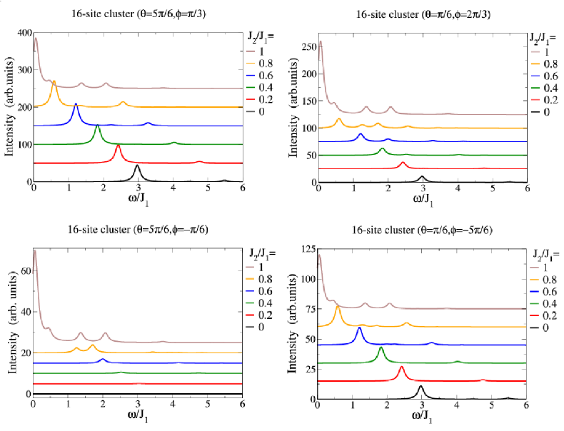
Figure 2: Exact diagonalizations on a 16-site cluster. Raman spectra for various values of $(\theta,\phi)$ and $J_{2}/J_{1}$. The bottom (top) left panel would correspond to $A_{1g}$ ($B_{1g}$) polarization on the square lattice in the case $J_{2}=0)$.

The bottom left panel of Fig. 2 shows, for $J_{2}=0$, the well known zero A_1g Raman scattering on a square lattice, since the scattering operator commutes with the Hamiltonian [9]. As $J_{2}$ increases non-commuting contribution to the scattering intensity increases and the spectrum develops more structure. For the bottom right panel, a weak intensity if observe because the scattering operator does not commute with the Hamiltonian even for $J_{2}=0$.
From the Hamiltonian in Eq. 2, it is obvious that the ground state will depend on the ratio $J_{2}/J_{1}$, ranging from a Néel-like order on the square lattice when $J_{2}=0$, to a three sublattice long-range order for $J_{2}=J_{1}$ [10, 11, 12]. These different type of order are characterized by different magnon dispersions, therefore the Raman spectra is expected to depend on $J_{2}/J_{1}$. In a recent paper, Zheng et al. [3] showed, using series expansions, that the magnon dispersion for the anisotropic triangular lattice Heisenberg model exhibits a roton-like minimum. This local minimum sits at the $(\pi,0)$ point for a square lattice with one diagonal bond and is getting softer as the $J_{2}$-diagonal frustrating coupling increases. In the case of the standard square lattice, for the B_1g channel with crossed polarizations, the electromagnetic field couples to excitations along the $(\pi,0)$ direction. We note from [3] that this softening is a multi-magnon process that cannot be captured to lowest order in a 1/S expansion. However, since we are using exact-diagonalization which, by its nature, treats processes for the length scale considered exactly, we are able to detect indications of this softening. For specificity, consider the B_1g channel in the top left-hand panel of Fig. 2. A signature of the softening of the magnon excitation is clearly manifest as the frustration ratio $f=J_{2}/J_{1}$ is increased from zero, with a shift of the spectral weight, and the main peak moving from $\omega\approx 3J_{1}$ when $J_{2}=0$ to $\omega\approx 0.6J_{1}$ when $J_{2}=0.8J_{1}$.

5 Conclusions and perspectives

The results presented here show how frustration can dramatically alter the Raman spectrum of an otherwise non-frustrated system. In particular, we observe a frustration-driven spectral downshift, the landmark feature of frustrated systems. This shift is another indicator of the frustration-induced softening of the magnon dispersion recently predicted by others. From a strictly theoretical point of view, the analysis above sets the stage for a more complete approach. Some exact-diagonalizations on larger cluster and a spin-wave approach including magnon-magnon interactions, along the lines pursued for the square lattice [13, 14], are currently being carried out.

References

References

- [1] R. Coldea et al., Phys. Rev. Lett. 88, 137203 (2002) ; R. Coldea et al., Phys. Rev. B 68, 134424 (2003)
- [2] Y. Shimizu et al., Phys. Rev. Lett. 91, 107001 (2003)
- [3] W. Zheng et al., Phys. Rev. Lett. 96, 057201 (2006)
- [4] P. A. Fleury and R. Loudon, Phys. Rev. 166, 514 (1968)
- [5] B. S. Shastry and B. I. Shraiman, Int. Jour. Mod. Phys. B5, 365 (1991) ; B. S. Shastry and B. I. Shraiman Phys. Rev. Lett. 65, 1068 (1990)
- [6] P. Lemmens et al., Phys. Rev. Lett. 96, 167204 (2006)
- [7] D. Qian et al., Phys. Rev. Lett. 96, 216405 (2006)
- [8] A. W. Sandvik, S. Capponi, D. Poilblanc and E. Dagotto, Phys. Rev. B 57, 8478 (1998)
- [9] P. J. Freitas and R. R. P. Singh, Phys. Rev. B 62, 5525 (2000)
- [10] Z. Weihong, R. H. McKenzie, R. R. P. Singh, Phys. Rev. B 59, 14367 (1999)
- [11] C. H. Chung, J. B. Marston, R. H. McKenzie, J. Phys. Condens. Matter 13, 5159-5181 (2001)
- [12] B. Bernu, C. Lhuillier and L. Pierre, Phys. Rev. B 50, 10048 (1994)
- [13] C. M. Canali and S. M. Girvin, Phys. Rev. B 45, 7127 (1992) ;
- [14] A. V. Chubukov and D. M. Frenkel, Phys. Rev. B 52, 9760 (1995).