Granular circulation in a cylindrical pan: simulations of reversing radial and tangential flows

Abstract

Granular flows due to simultaneous vertical and horizontal excitations of a flat-bottomed cylindrical pan are investigated using event-driven molecular dynamics simulations. In agreement with recent experimental results, we observe a transition from a solid-like state, to a fluidized state in which circulatory flow occurs simultaneously in the radial and tangential directions. By going beyond the range of conditions explored experimentally, we find that each of these circulations reverse their direction as a function of the control parameters of the motion. We numerically evaluate the dynamical phase diagram for this system and show, using a simple model, that the solid-fluid transition can be understood in terms of a critical value of the radial acceleration of the pan bottom; and that the circulation reversals are controlled by the phase shift relating the horizontal and vertical components of the vibrations. We also discuss the crucial role played by the geometry of the boundary conditions, and point out a relationship of the circulation observed here and the flows generated in vibratory conveyors.

I Introduction

In a recent experimental work, Sistla, et al. sistla02 observed a novel granular circulation occurring in a flat-bottomed cylindrical container (or “pan”) subjected to coupled horizontal and vertical vibrations. The apparatus studied was a commonly available industrial device used mainly for sieving and polishing of granular particles. Of particular interest was the appearance of a “toroidal” circulation, in which granular flow occurred simultaneously in the tangential direction (i.e. a circulation in the horizontal plane about the vertical axis), as well as radially (i.e. particles flowed outward along the bottom surface and then back to the center of the pan along the top surface of the granular bed). In this mode, the trajectory of a single particle would therefore approximate a helix on the surface of a torus. Among several other phenomena, it was noted that the direction of the tangential flow was, under most of the conditions explored, opposite to that of the orbital motion of the center of the pan. However, under some conditions, the tangential flow would reverse direction, and move in the same direction as the pan center. The authors noted that the phase shift relating the vertical and horizontal vibrations seemed to control this reversal. Whatever their origin, these phenomena indicate a non-trivial interplay of the horizontal and vertical vibrations, and their interaction with the granular bed. Since the bottom surface of the pan in the apparatus was a rough wire screen, the authors of Ref. sistla02 suggested that entrainment of particles to the motion of the bottom surface might play an important role in establishing the direction of the observed granular circulations.

Motivated by the complexity of phenomena observed in Ref. sistla02 , we present here a computer simulation study of a granular matter system enclosed in the same container geometry as in Ref. sistla02 , and subjected to a similar form of horizontal and vertical vibration. As we will show below, we are able to reproduce the major dynamical modes of the granular bed observed experimentally. We also explore the dynamical behavior beyond the range studied experimentally, and discover an entire family of circulation reversal transitions, affecting both the tangential and radial circulations. By analyzing the interaction of the particle bed with the rough pan bottom, we are able to show how particle entrainment, along with the phase shift relating the horizontal and vertical vibrations, together conspire to control the direction of the observed circulations.

Although most previous work on granular circulation has focussed on either purely vertical or purely horizontal vibrations (see e.g. Refs. JN92 ; BD92 ; M94 ; JNB96 ; JNBpt96 ; D98 ), a growing body of research is emerging related to granular flows generated by simultaneous horizontal and vertical vibrations and/or shear TB98 ; King et al. (2000); DB05 ; Gotzendorfer et al. (2005). This is significant since most industrial devices (e.g. seives, grinders and vibratory conveyors) generate both vertical and horizontal excitations. Understanding how the fundamental physical mechanisms of granular flow relate to practical applications therefore depends on the detailed examination of systems, such as the one studied here, having excitations in more than one dimension. As in our findings, these earlier works on simultaneous vertical and horizontal vibrations also point out the significance of the phase shift between the two types of excitation as being an important control parameter.

The cylindical geometry of our system (with the cylinder axis oriented vertically) is also a distinguishing aspect of the present work. A few recent works have studied granular flow in annular troughs, and have also observed tangential circulations similar to those studied here Grochowski et al. (2004); hor and Linz (2005). However, Ref. sistla02 and the present study are, to our knowledge, the first works to address radial circulation in this geometry.

II Description of the pan motion

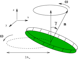
Figure 1: Geometry and parameters describing the pan motion. All symbols are defined in the text.

The shape of the flat-bottomed cylindrical pan and its motion are illustrated in Fig. 1. The forcing motion we impose on the pan in our simulations is based on the motion observed in the experimental apparatus used in Ref. sistla02 . This motion is complex and is described in detail in this section.

We assume that the pan is a rigid body. Let ${\bf n}$ be the normal vector to the bottom of the pan, rooted at the center of the bottom surface. The motion of the pan can then be described as a superposition of two motions: (i) a precession of ${\bf n}$ about the vertical axis with angular frequency $\omega$, and with ${\bf n}$ tilted at a constant angle $\gamma$ with respect to the vertical; and (ii), a circular motion of the center of the pan in the horizontal plane, of amplitude $A_{c}$ and also at frequency $\omega$. Note that the direction of rotation of both motions is always the same, and in our simulations, chosen to be counter-clockwise.

In this motion, the time evolution of the point $(x_{c},y_{c},z_{c})$ at the center of the pan bottom has only horizontal components which are non-zero, and thus can be described in the lab frame by,

$$z_{c} = 0$$

$$x_{c} = A_{c}\,\cos(\omega t)$$ (1)

$$y_{c} = A_{c}\,\sin(\omega t)$$

Also in the lab frame, the components of the vector ${\bf n}$ are given by,

$$n_{x} = \sin(\gamma)\,\cos(\omega t-\alpha_{xz})$$

$$n_{y} = \sin(\gamma)\,\sin(\omega t-\alpha_{xz})$$ (2)

$$n_{z} = \cos(\gamma)$$

where $\alpha_{xz}$ is the phase shift between the circular motion of the pan center, and the precessional motion of ${\bf n}$.

In order to analyze the behavior of the granular particles in the moving pan, we also need to derive expressions describing the motion, in the lab frame, of an arbitrary point $P$ fixed on the pan bottom. Let $(x_{p},y_{p})$ be the Cartesian coordinates of $P$ in a frame of reference fixed to, and lying in the plane of, the pan bottom. The coordinates of $P$ in the lab frame, $(x,y,z)$, are then given by,

$$x(t) = x_{p}+A_{c}\cos(\omega t)$$ (3)

$$y(t) = y_{p}+A_{c}\sin(\omega t)$$ (4)

$$z(t) = -\frac{x_{p}n_{x}+y_{p}n_{y}}{n_{z}}$$ (5)

The expression for $z(t)$ above is determined from the condition that the pan is a rigid body, and from the orthogonality of the vectors ${\bf n}$ and ${\bf p}$, where ${\bf p}$ is the vector from the center of the pan bottom to the point $P$, in the pan frame. If we express $(x_{p},y_{p})$ in terms of a polar coordinate system $(r,\theta)$ that is also fixed in the pan frame, then $x_{p}=r\cos\theta$ and $y_{p}=r\sin\theta$, where $r=\sqrt{x_{p}^{2}+y_{p}^{2}}$. Using the trigonometric identity $\cos\alpha\cos\beta+\sin\alpha\sin\beta=\cos(\alpha-\beta)$, Eq. 5 can be rewritten as,

$$z(t)=-r\,\tan(\gamma)\,\cos(\omega t-\alpha_{xz}-\theta)$$ (6)

Note that in Ref. sistla02 , $A_{c}$ is referred to as $x_{max}=y_{max}$ and the maximum vertical amplitude of vibration $R\sin\gamma$, where $R$ is the radius of the pan, is referred to as $z_{max}$. With these changes of notation, the representation of the pan motion presented in Eqs. 3, 4 and 6 is consistent with Eqs. 1-3 of reference sistla02 .

III Numerical Simulations

III.1 Event Driven Algorithm

The event driven algorithm Lubachevsky (1991) used in our simulations has proved very effective in simulating agitated granular matter. For example, simulations of standing wave patterns in 3D vertically oscillated granular layers Bizon et al. (1998a) show remarkable agreement with experiments. The algorithm itself is well described elsewhere (see e.g. Refs. Lubachevsky (1991, 1992)). In short, it involves five steps: (i) the calculation of collisions times between particles and between particles and walls; (ii) determining which pair of objects are next to collide by finding the minimum of the collision times; (iii) evolving the system forward in time to the next-to-occur collision by changing the coordinates and velocities of all particles according to the equations of motion of free particles in a gravitational field; (iv) changing the velocities of the two colliding particles (or of a particle hitting a wall) according to the conservation of linear and angular momentum and a specified rule for the dissipation of energy in the collision; and (v), returning to step (i). The algorithm assumes that interactions occur only through instantaneous binary collisions.

We have adapted this algorithm to our specific system by implementing the interactions between particles and moving walls of a cylindrical flat-bottomed container in a manner that is consistent with hard sphere dynamics. As described below, we give special care to the implementation of roughness of the bottom surface of the container. We have tested several models for the interaction between particles and a rough bottom plate and decide on the one presented below because of its simplicity combined with its efficiency.

III.2 System Parameters

In all our simulations the particles are monodisperse spheres of diameter $\sigma$ possessing both linear and angular momentum. Otherwise, our numerical model has a fairly large number of parameters that have to be set so that the model can be validated against the experimental results of Ref. sistla02 . In the following we organize these into three groups: dissipative, system size, and forcing parameters.

Dissipative Parameters: These parameters control the way energy is dissipated in the system. We implement inelastic collisions between particles in the manner described in Walton (1993). The collisions between particles are thus dependent on the coefficient of restitution $e$, defined as the ratio of the normal components of the relative velocities of two colliding particles before and after the collision; the rotational coefficient of restitution $\beta$, defined as the ratio of tangential components of relative surface velocities of colliding particles before and after the collision; and the coefficient of friction $\mu$ for the material from which the particles are made.

We set $e$ to be velocity dependent in the following way:

$$e(v_{n})=\left\{\begin{array}[]{ll}1-Bv_{n}^{3/4},&v_{n}<v_{o}\\ \epsilon,&v_{n}>v_{o}\end{array}\right.$$ (7)

Here $v_{n}$ is the component of relative velocity along the line joining particle centers, $B=(1-\epsilon)v_{o}^{-3/4},v_{o}=\sqrt{g\sigma}$ is a characteristic velocity of the particles, $g$ is the acceleration due to gravity, and $\epsilon$ is a tunable parameter of the simulations. Decreasing $\epsilon$ increases the energy dissipated during each collision. The advantages of this model for the coefficient of restitution are discussed and demonstrated in Refs. Shattuck et al. (1997); Bizon et al. (1998a, b); Goldman et al. (1998); Bizon et al. (1999); BK05 . We have set $\epsilon=0.6$, because this value gives the best agreement in terms of particle compaction observed in similarly agitated states in experiments with nylon balls and in our simulations.

The dissipation of rotational kinetic energy due to colliding particles is controlled by $\beta$. As validated in Ref. Walton (1993), the dependence of $\beta$ on the relative particle velocities and on $\mu$ depends on the value of the threshold parameter $\beta_{o}$ that controls the choice between a rolling or sliding solution in a given particle-particle collisions. Ref. Walton (1993) suggests that $\beta_{o}=0.35$ is a reasonable choice for plastic sphere collisions based on comparison with experiments. We use this value in all our simulations. We have set $\mu=0.5$ in all our simulations based on the findings of Ref. Bizon et al. (1998a).

The dissipation of energy in collisions between particles and the side walls and the bottom of the container is determined by the same set of parameters ($\epsilon$, $\mu$, and $\beta_{o}$) as in particle-particle collisions. For the case of collisions between particles and the side walls we have observed, however, that the simulated system’s behavior is not detectably changed when using $\epsilon=1$ (elastic collisions) instead of $\epsilon<1$ (inelastic collisions). Thus, in all our simulations we set $\epsilon=1$ for collisions between particles and the side walls.

Special attention is given to the implementation of momentum transfer and dissipation of energy in collisions between particles and the rough bottom of the container. Instead of using three dissipative parameters as in particle-particle collisions, we implement a one-parameter model as follows. In the reference frame of the moving pan, the particle strikes the bottom plate with a relative incident velocity $\bf{u}$ at the contact point where the surface normal is $\bf{n}$. The particle is reflected from the surface with relative velocity ${\bf v}=e(|{\bf u}|)[{\bf u}-(2{\bf u\cdot n}){\bf n}]$ where $e(|{\bf u}|)$ has the same form as Eq. 7, except that it is a function of the absolute value of the incident velocity and not just the normal component. Thus, if not for the factor of $e(|{\bf u}|)$, the particle-bottom collision would be elastic. The decrease of all three components of the reflected velocity by the factor $e(|{\bf u}|)$ is essential here for modeling the entrainment of particles by the rough bottom surface. Indeed, the effect of this decrease is that the particle’s velocity (in the lab frame) after the collision tends to be more similar to the velocity of the rough bottom surface at the point of contact, than before the collision. This, in turn, makes the choice of the reflection direction of little importance. Statistically the average direction of reflection must be in the plane of the vectors $\bf{u}$ and $\bf{n}$, as it is in our model. Thus the only parameter of our model for the rough bottom surface is $\epsilon$ in Eq. 7. We have tested several values of this parameter in the range between $0.6$ and $0.9$. Lower values of $\epsilon$ provide better entrainment of particles by the bottom surface, but at the same time make the average collision time close to the surface so small that roundoff errors render the simulations unphysical. Thus, we have adopted a value of $\epsilon=0.8$ as a compromise that realizes particle entrainment at the bottom surface as well as well-behaved numerical simulations.

System Size Parameters: These parameters include the particle diameter $\sigma$, number of particles $N$ and the radius of pan $R$. The layer depth $H$ can be estimated assuming the volume fraction $\Phi\equiv(N\frac{1}{6}\pi\sigma^{3})/(\pi R^{2}H)$ is equal to the experimentally determined Bizon et al. (1998a) value of $0.58$. For example, in the laboratory experiments of Ref. sistla02 using nylon balls, a 30 kg load of particles (each weighing 0.9 g and 11.5 mm in diameter) in a pan of radius 0.381 m gave $H/\sigma=8.7$ for the layer depth. In the present simulations we set the number of particles to either $N=2175$ or $N=15000$. In the first case we have $R/\sigma=12.5$ and $H/\sigma=4.0$, and in the second case we have $R/\sigma=33$ and also $H/\sigma=4.0$. Although the layer depth in our simulations is smaller than in the experiments, as we will show below, we are able to reproduce the main features of the dynamical behavior observed in experiments. In this work we have chosen to present the results for only the smaller system size ($N=2175$) because the shorter computing times allow for larger statistical sampling. Our tests of the system behavior using the larger number of particles indicates that the results are qualitatively the same as for the smaller system.

Forcing Parameters: The frequency of vibrations $f=\omega/2\pi$, the phase shift $\alpha_{xz}$, the amplitude of horizontal vibrations $A_{c}$, and the tilt angle $\gamma$, were introduced in Section II. For all results presented here we consider the set $(f,\alpha_{xz})$ as the independent variables and we study the system behavior as a function of this set, with all other parameters fixed. Table 1 shows the values (or range of values) of the forcing and system size parameters studied here, compared to those examined in the experiments of Ref. sistla02 .

As stated above, we conduct simulations on a system that is smaller than that of the experiments in order to allow us to study as wide a range of dynamical states as possible. Since the pan radius $R$ in our simulations is therefore smaller than in the experiments, we have set the value of the tilt angle $\gamma$ to a larger value, such that the maximum amplitude of vertical motion at the edge of the pan $z_{max}=R\,\,\tan\gamma$ is approximately the same as in the experiments. We also find that we must set the value of $A_{c}$, the amplitude of the horizontal motion, to a larger value (compared to experiments) in order to achieve a robust entrainment of the particles near the rough bottom surface. This suggests that the model of surface roughness used in our simulations is less effective in entraining particle motion than the real system.

Table 1: Comparison of simulation parameters used in the present work, and experimental parameters from Ref. sistla02 .

	$f$ (Hz)	$\alpha_{xz}$	$A_{c}/\sigma$	$\gamma$	$R/\sigma$	$H/\sigma$
exp	10 - 20	0∘ - 150∘	0.09 - 0.17	0.15∘ - 0.60∘	33.1	8.7
sim	5 - 55	0∘ - 360∘	0.5	1.5∘	12.5	4.0

IV Results

IV.1 Dynamical modes

Figure 2: Velocity field for toroidal motion at $f=25.5$ Hz and $\alpha_{xz}=144^{\circ}$. Top panel: the velocities of particles in the layer nearest the bottom surface, viewed from above. Each arrow length is proportional to the magnitude of the average velocity corresponding to each grid location. Note that the pan center always rotates in the counter-clockwise direction in our simulations, but that under the conditions of the state shown here, the tangential flow is clockwise. Bottom panel: the velocity field of particles of the same system in a vertical cross section passing through the pan center. Here, all arrow lengths are fixed to a constant, and do not represent the magnitude of the average velocities. $r_{o}$ and $h_{o}$ approximately locate the center of circulation of the radial flow.

Using the set of parameters described in the previous section, we study the behavior of the system as a function of $f$ and $\alpha_{xz}$. We conduct simulations for 15 different frequencies, in the range between 5 and 55 Hz. For each $f$ we set the phase angle $\alpha_{xz}$ to at least 20 different values in the range $0-360^{\circ}$. We thereby analyze a total of more then 300 state points. In the range of $f$ considered here, the motion settles into a steady state in less than 1.0 s of physical simulation time, which corresponds to approximately 10-50 revolutions of the pan, depending on $f$. To ensure equilibration, we therefore run each simulation for at least 2 s before starting to accumulate averages.

From a visual examination of animations of the steady-state behavior, we find that at fixed $\alpha_{xz}$, three main regimes of dynamical behavior occur as $f$ increases: (i) At small $f$, we observe a solid-like heap state that undergoes a collective tangential rotation about the vertical axis. This is qualitatively the same behavior observed at small $f$ in Ref. sistla02 . (ii) At larger $f$, typically in the range of 15-20 Hz, a transition occurs to a “toroidal” motion, having simultaneous tangential and radial circulations, which is also very similar to that observed experimentally. (iii) At large $f$, the toroidal state crosses over to a gas-like state in which the particles have a sufficiently large kinetic energy that gravity cannot maintain the particles in a dense bed at the bottom of the pan; in this regime, the particles spread out over the entire system volume. This crossover occurs in the range of $f$ between 30 and 48 Hz, depending on $\alpha_{xz}$.

The simultaneous tangential and radial circulations occurring in the toroidal regime are shown in Fig. 2. The top panel of Fig. 2 shows the velocity field for the particles in a horizontal layer that is adjacent to the pan bottom. The bottom panel shows the velocity field for particles in a vertical plane passing through the center of the pan. In these vector field plots we display the velocity vectors within the corresponding volume of space averaged over a local volume of $\sigma^{3}$ and over 400 snapshots of the system taken 0.001 s apart. Therefore, the total averaging time (0.4 s) is much longer than the period of oscillation of the pan in the range of $f$ studied here.

IV.2 Phase diagram

Figure 3: $\omega_{r}$ (triangles) and $\omega_{t}$ (circles) as a function of $\alpha_{xz}$ at various $f$. To facilitate comparison, $\omega_{r}$ values are multiplied by 30, and $\omega_{t}$ values by 1.5.

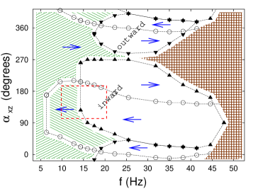
Figure 4: Phase diagram of dynamical modes found in simulations. The solid-like heap state occurs at low $f$, in the diagonally striped areas. The domain of the gas-like state at high $f$ is denoted by the square lattice pattern. The remaining white areas, bounded by triangles, indicate the domains in which the toroidal circulation is observed. The label “inward” indicates the region where the radial flow is such that particles travel toward the center along the top surface of the bed. The label “outward” indicates the region where the radial flow is such that particles travel away from the center along the top surface of the bed. For both the heap and toroidal states, the line that connects the open circles indicates a change of direction of the tangential flow. Left (right) arrows indicate that the direction of the tangential flow is against (with) the direction of the pan rotation. The dashed rectangle shows the approximate region corresponding to the experiments of Ref. sistla02 . Error bars for the boundaries of the toroidal domains (triangles) are of the size of the symbol for low $f$ and increase to up to three times the size of the symbol for high $f$.

Figure 5: Velocity field in a vertical cross section passing through the pan center, illustrating outward radial flow, occurring at $f=27$ Hz and $\alpha_{xz}=0^{\circ}$.

We next seek to create a dynamical phase diagram of the system, i.e. to subdivide the plane of $f$ and $\alpha_{xz}$ into domains according to where each of the observed dynamical modes occurs. To do so, we quantify the state of circulation in the granular bed using two measures of the average velocity of the particles.

The first measure, $\omega_{t}$, quantifies the tangential circulation and is the average angular velocity of particles in the horizontal plane around the vertical line of symmetry:

$$\omega_{t}=\frac{1}{N}\sum_{i}\frac{v_{t,i}}{d_{i}}=\frac{1}{N}\sum_{i}\frac{1}{d_{i}}\,{\bf{v}}_{i}\cdot(\hat{\bf{k}}\times\hat{\bf{r}}_{i})$$ (8)

Here, $v_{t,i}$ is the tangential component of ${\bf v}_{i}$, the velocity of particle $i$, about the vertical axis. $d_{i}$ is the perpendicular distance from a particle $i$ to the $z$-axis of the lab frame; $\hat{\bf{k}}$ is the unit vector pointing along the $z$-axis of the lab frame; and $\hat{\bf{r}}_{i}$ is the radial unit vector at the position of particle $i$ in the lab frame.

The second measure quantifies the radial circulation. We define this measure, $\omega_{r}$, as the average angular velocity of particles about the curved axis that forms a horizontal circle of radius $r_{o}$ and elevated above the bottom of the pan at a distance $h_{o}$. As illustrated in the lower panel of Fig. 2, if we choose $r_{o}=0.75R$ and $h_{o}=0.75H$, we find that this curved axis approximately coincides with the center of the radial circulation observed in our simulations. $\omega_{r}$ is then given by,

$$\omega_{r}=\frac{1}{N}\sum_{i}\frac{v_{r,i}}{a_{i}}=\frac{1}{N}\sum_{i}\frac{1}{a_{i}}\,{\bf{v}}_{i}\cdot(\hat{\bf{t}}_{i}\times\hat{\bf{a}}_{i})$$ (9)

Here $v_{r,i}$ is the tangential component of ${\bf v}_{i}$, in a vertical plane, with respect the circulation center defined by $r_{o}$ and $h_{o}$; and $\hat{\bf{t}}_{i}=(\hat{\bf{k}}\times\hat{\bf{r}}_{i})$. $\hat{\bf{a}}_{i}$ and $a_{i}$ are respectively the direction and magnitude of the vector ${\bf{a}}_{i}={\bf{r}}_{i}-(h_{o}\hat{\bf{k}}+r_{o}\hat{\bf{r}}_{i})$ which defines the position of particle $i$ with respect to the center of circulation in the vertical plane.

Examples of the behavior of $\omega_{t}$ and $\omega_{r}$, as a function of $\alpha_{xz}$ at various fixed $f$, are shown in Fig. 3. In Fig. 3(a), we see that $\omega_{r}=0$ for $\alpha_{xz}<90^{\circ}$, becomes non-zero for higher $\alpha_{xz}$, but then returns to zero as $\alpha_{xz}$ approaches $360^{\circ}$. Based on our visual observations of the computer animations, the heap state exhibits no radial circulation, and so the progression of behavior of $\omega_{r}$ in Fig. 3(a) reflects the transition first from the heap to the toroidal mode, and then back again, as a function of $\alpha_{xz}$. On the other hand, we see that $\omega_{t}$ varies smoothly as a function of $\alpha_{xz}$ in Fig. 3(a), reflecting the fact that tangential circulation is common to both the heap and toroidal modes. Based on these observations, for the purpose of constructing a phase diagram, we define the toroidal state as that in which $\omega_{r}$ is clearly different from zero. We also note that the variation of $\omega_{t}$ and $\omega_{r}$ with $\alpha_{xz}$ is approximately sinusoidal, with the behavior of $\omega_{r}$ lagging that of $\omega_{t}$ by about $90^{\circ}$. We will return to this behavior in the next section.

The resulting phase diagram is shown in Fig. 4. The most notable behavior of the observations summarized in Figs. 3 and 4 is that we find that both the radial and tangential circulations reverse their direction as a function (primarily) of $\alpha_{xz}$, as indicated by the occurrence of both positive and negative values of $\omega_{t}$ and $\omega_{r}$ in Fig. 3. The result is a rich and highly controllable spectrum of dynamical behavior: at low $f$, we see heap states that rotate either clockwise or counter-clockwise (viewed from above); at higher $f$, toroidal states with any combination of clockwise or counter-clockwise tangential circulation, and inward or outward radial circulation (based on the flow direction on the upper free surface) can be realized. The velocity field of a system with an outward radial circulation is shown in Fig. 5. In addition, the magnitudes of both $\omega_{t}$ and $\omega_{r}$ can be readily tuned through their dependence on $f$ and $\alpha_{xz}$.

The phase behavior shown in Fig. 4 is in quantitative agreement with the experimental results of Ref. sistla02 for the boundary between the heap and toriodal modes. The forcing conditions studied in Ref. sistla02 correspond approximately to $10<f<20$ and $100^{\circ}<\alpha_{xz}<190^{\circ}$, in the notation of this work. In this range, the tangential circulation is (almost always) in the same direction for both the heap and toroidal modes, and, as in experiments, is opposite to the direction the pan center rotates. The exception, in both simulations and experiments, occurs for small values of both $f$ and $\alpha_{xz}$, where the tangential circulation occurs in the same direction as the pan center rotates. Since the experiments only studied a small fraction of the phase diagram explored here, the reversal of the radial circulation was not observed in experiments, but is revealed here, along with the complete demarcation of the reversal boundary for the tangential circulation.

We note that the more subtle modifications of the toroidal mode observed experimentally (the “surface waves” and “sectors” described in Ref. sistla02 ) are not observed here, suggesting that these phenomena depend on aspects of the motion and/or particle interactions that are not modeled in the present simulations. One possibility is that these modifications of the toroidal mode are due to variations of the pan motion from a perfect sinusoid. As indicated in Ref. sistla02 , the experimental apparatus was not perfectly symmetrical, and the measured motion indicated the presence of a weak pattern of beats superimposed on the principal motion. While it is possible that the experimentally observed surface waves and sectors had there origin in these additional components of the motion, more research, beyond the scope of that described here, would be required to clarify this issue.

V Origins of observed flows

In this section, we discuss some of the physical mechanisms that may underlie the behavior noted so far. We focus in turn on two questions: (i) Why do the horizontal and radial circulations reverse their direction as a function of $\alpha_{xz}$? (ii) What parameters determine the onset of heap-to-toroidal flow?

V.1 Circulation reversals

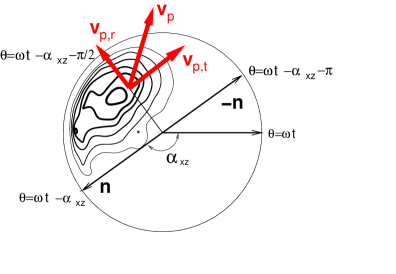
Figure 6: Interrelationship of the zone of contact between the granular bed and the pan bottom, and the motion of the pan, as viewed from above, for $f=23.4$ Hz, $\alpha_{xz}=144^{\circ}$. The contours are lines along which the average momentum change of particles colliding with the bottom surface is constant. The vector labeled ${\bf n}$ is the projection of the pan normal vector into the horizontal plane, and indicates the direction along which the vertical displacement of the pan is most negative. The vector labelled ${\bf-n}$ therefore indicates the direction along which the vertical displacement of the pan is most positive. Since the pan center orbits counter-clockwise in the horizontal plane, the half circle above and to the left of the bisector formed by ${\bf n}$ and ${\bf-n}$ is that half of the bottom surface that is rising. The zone of contact, located in the region around the center of the momentum-change contours, is located on the rising side of the pan bottom, and has its center near the direction $\theta_{o}=\omega t-\alpha_{xz}-\pi/2$. The horizontal “pushing velocity” of the bottom pan surface, ${\bf v}_{p}$, and its polar component vectors, are also shown.

In order to clarify the nature of the interaction between the granular bed and the moving pan, we first examine the nature of the contact between the two as a function of time. To determine where and when the bed is in contact with the pan as a function of time, we subdivide the pan bottom into a grid of squares of area $\sigma^{2}$. Over a time interval of 0.05 of the period of revolution of the pan, we then find the average change of momentum of particles colliding with the pan bottom in each grid square. This provides a measure of the instantaneous pressure exerted by the bed on each area element of the pan bottom. When the system is in a dynamical steady state, we can average over “snapshots” of the pressure distribution on the pan bottom at different times by rotating each snapshot around the pan center such that the direction given by $\theta=\omega t$ always points along the positive $x$-axis. Pressure contours resulting from this averaging process over a total time of 300 revolutions of the pan are shown in Fig. 6 for the case $f=23.4$ Hz, $\alpha_{xz}=144^{\circ}$. The pressure contours show that a well-defined “zone of contact” exists between the granular bed and the pan bottom at a particular angular position. Similar results are obtained at other values of $f$ and $\alpha_{xz}$, and differ only in the angular position of the zone of contact.

We find that $\theta_{o}$, the angular position of the center of the zone of contact is, in all cases examined, close to the value,

$$\theta_{o}=\omega t-\alpha_{xz}-\pi/2$$ (10)

A relatively simple rationale supports this expression: We expect that the contact between the bed and the pan occurs on that side of the pan which is rising from its maximum negative displacement in the $z$ direction to its maximum positive displacement. As shown in Fig. 6, when the normal vector of the pan ${\bf n}$ is precessing counter-clockwise, the “rising” half of the pan bottom is identified by those values of $\theta$ such that,

$$0<(\omega t-\alpha_{xz}-\theta)<\pi$$ (11)

We see from Fig. 6 that the maximum pressure of the zone of contact is approximately in the middle of this half of the pan bottom, the angular position of which is given approximately by Eq. 10.

Next we note that we have modeled the pan bottom as a rough surface that entrains the motion of particles that collide with it; i.e. particles tend to have a post-collision velocity with a direction similar to that of the surface element of the pan bottom that they strike. Since the contact between the granular bed and the pan bottom is localized to the zone of contact, we expect that the velocity of the surface elements at the angular position given by Eq. 10 will have a significant influence on the direction of flow of the bed. Let us define the “pushing velocity” ${\bf v}_{p}$ as the component of the pan bottom velocity in the horizontal plane at $\theta=\theta_{o}$. The time derivatives of Eqs. 3 and 4 give us the $x$ and $y$ components of ${\bf v}_{p}$: $v_{p,x}=-A_{c}\omega\sin(\omega t)$ and $v_{p,y}=A_{c}\omega\cos(\omega t)$. Converting these Cartesian components to those in a polar coordinate system gives the radial and tangential components of ${\bf v}_{p}$. The desired radial unit vector is $\hat{\bf r}=(\cos\theta_{o},\sin\theta_{o})$ and the tangential unit vector is $\hat{\bf t}=[\cos(\theta_{o}+\pi/2),\sin(\theta_{o}+\pi/2)]$. The radial and tangential components of ${\bf v}_{p}$ are therefore given by,

$$v_{p,r}={\bf v}_{p}{\bf\cdot\hat{r}}=-A_{c}\omega\cos(\alpha_{xz})$$ (12)

$$v_{p,t}={\bf v}_{p}{\bf\cdot\hat{t}}=-A_{c}\omega\sin(\alpha_{xz})$$ (13)

Comparing these expressions with the dependence of $\omega_{t}$ and $\omega_{r}$ on $\alpha_{xz}$ shown in Fig. 3 shows that there is a good correspondence between the polar components of ${\bf v}_{p}$ and the observed angular velocity of both the radial and tangential flows. $\omega_{t}$ shows an especially good match to a function proportional to $-\sin(\alpha_{xz})$. The correspondence of $\omega_{r}$ to $-\cos(\alpha_{xz})$ is complicated by the fact that $\omega_{r}=0$ in the heap state. However the observed trend for $\omega_{r}$ to lag $\omega_{t}$ by $90^{\circ}$ is consistent with the implications of Eqs. 12 and 13.

Overall, we therefore find that the assumption that the particles are entrained by the pan bottom in a specific zone of contact explains well the observed circulation. If the polar components of ${\bf v}_{p}$ drive the motion observed via $\omega_{t}$ and $\omega_{r}$, then Eqs. 12 and 13 predict the occurrence of both clockwise and counter-clockwise tangential circulations, as well as both inward and outward radial flows. In particular, Eqs. 12 and 13 also provide a basis for understanding why the tangential flow can be both the same as, or opposite to, the direction of rotation of the pan center. Most importantly, the dominant role of the phase shift $\alpha_{xz}$ in controlling the direction of the observed flows is confirmed.

V.2 Onset of toroidal flow

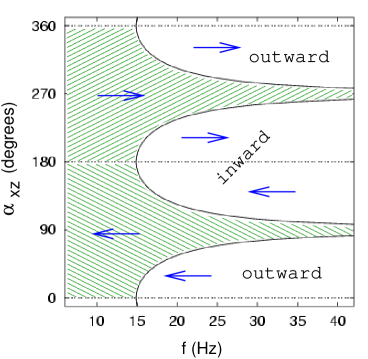
Figure 7: Model phase diagram based on Eqs. 12, 13 and 15. Solid lines indicate the onset of radial flow. Dotted lines indicate the change of direction of the tangential flow. Arrows and region labels have the same meaning as in Fig. 4.

Since both the heap and toroidal circulations exhibit tangential flow, understanding the onset of the toroidal mode requires us to understand the conditions required for the appearance of the radial circulation. This is a complex question, since the heap-to-toroidal boundary in Fig. 4 is clearly dependent both on $\alpha_{xz}$ and $f$.

To make a preliminary attempt to understand the dependence of the heap-to-toroidal boundary on $\alpha_{xz}$ and $f$, let us consider $a_{r}$, the maximum radial acceleration experienced by the particle bed, which drives the radial circulation observed in the toroidal mode. By analogy with many other systems exhibiting granular circulation, we expect that the onset of the toroidal mode occurs when $a_{r}$ exceeds a critical threshold large enough to sustain the radial circulation.

To estimate the scaling of $a_{r}$ with $\alpha_{xz}$ and $f$, we first assume that $a_{r}=A_{p}\omega^{2}$, where $A_{p}$ is the average displacement of the particle bed in the radial direction as it is pushed by the rough pan bottom. Given the correspondence between the components of the pushing velocity ${\bf v}_{p}$ and the circulation speeds $\omega_{t}$ and $\omega_{r}$ established in the previous section, we propose that $A_{p}$ is proportional to the product of $|v_{p,r}|$ and $\tau_{p}$, the time interval during which particles are exposed to the zone of contact. We also assume that $\tau_{p}$ is simply some fraction of the period of the pan motion, and so is proportional to $2\pi/\omega$. Combining these assumptions with the expression for $v_{p,r}$ in Eq. 12, we therefore can write,

$$a_{r}\propto\omega^{2}|\cos\alpha_{xz}|$$ (14)

If the onset of the heap-to-toroidal transition occurs at a critical value of $a_{r}=a_{r,c}$ then the corresponding critical angular frequency $\omega_{c}$ for the onset of radial circulation (and therefore toroidal flow) is given by,

$$\omega_{c}\propto\sqrt{\frac{a_{r,c}}{|\cos\alpha_{xz}|}}$$ (15)

Fig. 7 shows a plot of the critical frequency $f_{c}=\omega_{c}/2\pi$ in the $f$-$\alpha_{xz}$ plane, based on the proportionality expressed in Eq. 15, with the constant of proportionality chosen so that the mimimum onset frequency is $15$ Hz, as found in our simulations. Comparing Figs. 4 and 7 shows that the model expressed in Eq. 15 captures several qualitative features of the observed variation of the heap-to-toroidal transition: e.g. the occurrence of maxima in the transition boundary as a function of $\alpha_{xz}$; and the separation of the toroidal regime into two distinct domains, one exhibiting an inward radial flow, and one outward.

Clearly the approximations of this simple model should be refined if it is to have any quantitative predictive value. However, it does support the view that entrainment of the particle bed by the rough bottom is a key factor in determining the overall behavior of the system.

VI Discussion and Conclusion

Figure 8: Three types of boundary condition occurring in this system: (a) the periodic boundary condition involving the tangential flow; (b) the vertical wall obstacle encountered by the inward radial flow; (c) central “plume” obstacle encountered by the outward radial flow.

In summary, we have established the following picture for the dynamical behavior observed in our simulations, and to a large degree, in the experiments of Ref. sistla02 : The granular bed is excited by a rough horizontal surface that is undergoing both vertical and horizontal vibrations. The vertical vibrations impose a periodicity on the contact between the bed and the surface, and the horizontal vibrations push the granular bed only during the interval of contact. The phase shift relating the vertical and the horizontal components of the vibration determines the direction and strength of the horizontal pushing force applied by the rough surface on the bed. The result is a highly tunable spectrum of behavior, in which both tangential and radial circulations, in arbitrary combinations, can be generated.

The cylindrical geometry studied here plays an important underlying role in the granular flows we observe. The tangential circulation is in many ways similar to the kind of linear flow observed in vibratory conveyors hongler89 ; Sloot and Kruyt (1996), but wrapped around into a circle, creating in effect a periodic boundary condition. Indeed, a recent work studied the flow of granular matter in an annular vibratory conveyor and, as in our work, noted both the occurrence of a reversing tangential flow, and the controlling influence on this flow of the phase shift between vertical and horizontal vibrations Grochowski et al. (2004). The fact that the granular bed in our system encounters no obstacles as it moves about the center accounts for the ease with which the tangential flow occurs not only in the toroidal mode, but also the heap mode at very small $f$.

In contrast, the granular flow in the radial direction encounters a vertical barrier that it must surmount: either the outer wall in the case of the inward radial flow, or the central “plume” that is created when the granular particles are pushed toward the center in the outward radial flow (see Fig. 8). Here, the mechanism that drives the flow along the bottom surface is also similar to that of a vibratory conveyor, but with the complication that this driving force must be large enough to overcome the gravitational barrier imposed at the vertical boundary. This largely explains why the radial flow only occurs above a critical value of $f$.

Our results also demonstrate that complex dynamical modes observed in real (i.e. industrial) granular matter devices can, on the one hand, be understood using computer simulations; and on the other hand, the behavior observed in these real devices can reveal important fundamental principles (such as the role of the phase factor established here) relating to the creation and control of highly specialized granular flows.

- (1)
- (2) P. Sistla, O. Baran, Q. Chen, S. Fohanno, P.H. Poole and R.J. Martinuzzi, Phys. Rev. E 71, 011303 (2005)
- (3) H.M. Jaeger and S.R. Nagel, Science 255, 1523 (1992).
- (4) D. Bideau and J. Dodds, in Physics of Granular Media, (Les Houches Series, Nova Science Publishers, Commack, NY, 1991).
- (5) Granular Matter: An Interdisciplinary Approach, edited by A. Mehta (Springer-Verlag, New York, 1994).
- (6) H.M. Jaeger, S.R. Nagel, and R P. Behringer, Rev. Mod. Phys. 68, 1259 (1996).
- (7) H. M. Jaeger, S.R. Nagel, and R.P. Behringer, Physics Today 49, 32 (1996).
- (8) P.-G. de Gennes, Physica A 261, 267 (1998).
- (9) S.G.K. Tennakoon and R.P. Behringer, Phys. Rev. Lett. 81, 794 (1998).
- King et al. (2000) P. King, M. Swift, K. Benedict, and A. Routledge, Phys. Rev. E 62, 6982 (2000).
- (11) K.E. Daniels and R.P. Behringer, Phys. Rev. Lett. 94, 168001 (2005).
- Gotzendorfer et al. (2005) A. Gotzendorfer, J. Kreft, C. Kruelle, and I. Rehberg, Phys. Rev. Lett. 95, 135704 (2005).
- Grochowski et al. (2004) R. Grochowski, P. Walzel, M. Rouijaa, C. Kruelle, and I. Rehberg, Applied Phys. Lett. 84, 1019 (2004).
- hor and Linz (2005) H. E. hor and S. Linz, J. Stat. Mech. L02005 (2005).
- Lubachevsky (1991) B. D. Lubachevsky, J. of Comp. Phys. 94, 255 (1991).
- Bizon et al. (1998a) C. Bizon, M. D. Shattuck, J. B. Swift, W. D. McCormick, and H. L. Swinney, Phys. Rev. Lett. 80, 57 (1998a).
- Lubachevsky (1992) B. D. Lubachevsky, Int.J. in Computer Simulation 2, 373 (1992).
- Walton (1993) O. R. Walton, in Particulate two-phase flow, edited by M. C. Roco (Butterworth-Heinemann, Boston, 1993), p. 884.
- (19) O. Baran, L. Kondic, Phys. Fluids 17, 073304 (2005).
- Shattuck et al. (1997) M. D. Shattuck, C. Bizon, P. B. Umbanhowar, J. B. Swift, and H. L. Swinney, in Powders & Grains 97 (Balkema, Rotterdam, 1997).
- Bizon et al. (1998b) C. Bizon, M. D. Shattuck, J. R. de Bruyn, J. B. Swift, W. D. McCormick, and H. L. Swinney, J. Stat. Phys. 93, 449 (1998b).
- Goldman et al. (1998) D. Goldman, M. D. Shattuck, C. Bizon, W. D. McCormick, J. B. Swift, and H. L. Swinney, Phys. Rev. E 57, R4831 (1998).
- Bizon et al. (1999) C. Bizon, M. D. Shattuck, J. B. Swift, and H. L. Swinney, Phys. Rev. E 60, 4340 (1999).
- (24) M.-O. Hongler, P. Cartier and P. Flury, Phys. Lett. A 135, 106 (1989).
- Sloot and Kruyt (1996) E. Sloot and N. Kruyt, Powder Technology 87, 203 (1996).