Fractional charges and spin-charge separation in one-dimensional Wigner lattices

Abstract

We study density response $N(k,\omega)$ and one-particle spectra $A(k,\omega)$ for a Wigner lattice model at quarter filling using exact diagonalization. We investigate these observables for models with short and long-range electron-electron interaction and show that truncation of the electron repulsion can lead to very different results. The spectra show clear signatures of charge fractionalization into pairs of domain walls, whose interaction can be attractive or repulsive and is controlled by the formal fractional charges. In striking contrast to a bound exciton in $N(k,\omega)$, we find an antibound quasi-particle in $A(k,\omega)$, which undergoes spin-charge separation. We present a case of extreme particle-hole asymmetry, where photoemission shows spin-charge separation, while inverse photoemission exhibits an uncorrelated one-particle band.
$[$ published in Phys. Rev. B 75, 125116 (2007) $]$

I Introduction

In contrast to higher dimensions, where interacting electrons are renormalized into ‘Landau quasi-particles’ that near the Fermi surface still ‘look’ like electrons, drastic things can happen in one dimension. Maekawa01 The elementary excitations are collective ones involving many electrons, spin and charge separate and move independently of each other, as seen, e.g., in photoemission (PES) experiments.Kim06 Another case where many-body effects lead to an apparent splitting of elementary particles is quantum number fractionalization.Oshikawa06 Probably its most famous realization is the fractional quantum Hall effect.Lau83 Likewise, Peierls distorted Heeger88 and charge-ordered Hubbard78 ; Rice82 one-dimensional (1D) systems with degenerate ground states have fractionally charged solitons or domain walls as elementary excitations. In fact, quantum number fractionalization in one and two dimensions are intimately related.Seidel06 This Paper presents a study of dynamic observables for a model showing both effects, spin-charge separation as well as quantum number fractionalization.

When (long-range) Coulomb interaction is the dominant energy scale of a system, electrons try to minimize their energy by maximizing their distance and crystallize into a Wigner lattice (WL).Wigner34 Hubbard suggested this mechanism in the context of TCNQ charge-transfer salts Hubbard78 where it is, however, difficult to distinguish from a $4k_{F}$ charge-density wave driven by a Fermi surface instability. Hubbard78 ; Rice82 ; Nad06 As pointed out recently, Horsch05 longer-range hopping changes the Fermi-surface topology in doped edge-sharing CuO-chain compounds like Na_1+xCuO₂ Sofin05 and Ca_2+yY_2-yCu₅O₁₀, Kudo05 and this allows for a clear distinction between the Fermi-surface independent WL and the charge-density wave.

The elementary excitations of a WL consist of domain walls (DWs). Their fractional charge follows from topological arguments Jackiw75 ; Hubbard78 ; Rice82 and merely reflects the $n$-fold ground-state degeneracy at $x=m/n$ filling – it is not related to the specific form of the interaction that generates the charge order. After introducing the employed model Hamiltonian in Sec. II, we show in Sec. III that these fractional charges have direct physical meaning in a model with long-range Coulomb repulsion among electrons, because the resulting effective interaction between DWs is also Coulomb-like with a coupling constant determined by the fractional charges, their signs and distance. Consistent with the formal charges, the interaction is attractive for the charge response Valenzuela03 ; Fratini04 ; Mayr06 but repulsive for the electron addition (removal) process. We present and discuss charge response $N(q,\omega)$ and spectral densities $A(k,\omega)$ and show that the correspondence of formal DW charge and effective physical charge is tied to the long-range nature of Coulomb repulsion and absent for models with truncated electron-electron interaction.

As the energy scale for spin excitations is much smaller than either the Coulomb repulsion or the kinetic energy, previous investigations considered WL formation of spinless fermions. We will address the spin degree of freedom in Sec. IV and we will show how the interplay of spin and DW excitations leads to two different scenarios for the spectral density: (i) For nearest neighbor hopping, the coherent antibound DW excitation undergoes spin-charge separation in perfect analogy to an electron or hole added to the half-filled 1D Hubbard model. (ii) For 2nd neighbor hopping, we find striking differences between the particle and hole channels, where an electron behaves like an independent particle while a hole decays into a spinon and a holon.

II Model and methods

We study the Hubbard-Wigner Hamiltonian Mayr06

$$\begin{split}H&=t_{1}\sum_{i,\sigma}({c}^{\dagger}_{i,\sigma}{c}^{\phantom{\dagger}}_{i+1,\sigma}+\textrm{h.c.})+t_{2}\sum_{i,\sigma}({c}^{\dagger}_{i,\sigma}{c}^{\phantom{\dagger}}_{i+2,\sigma}+\textrm{h.c.})\\ &\quad+U\sum_{i}n_{i,\uparrow}n_{i,\downarrow}+\sum_{l=1}^{l_{\textrm{max}}}V_{l}\sum_{i}(n_{i}-\bar{n})(n_{i+l}-\bar{n})\;,\end{split}$$ (1)

with nearest neighbor (NN) and next nearest neighbor (NNN) hopping amplitudes $t_{1}$ and $t_{2}$. Operator ${c}^{\dagger}_{i,\sigma}$ (${c}^{\phantom{\dagger}}_{i,\sigma}$) creates (destroys) an electron with spin $\sigma$ at site $i$, $n^{\phantom{\dagger}}_{i,\sigma}={c}^{\dagger}_{i,\sigma}{c}^{\phantom{\dagger}}_{i,\sigma}$ and $n_{i}=n_{i,\uparrow}+n_{i,\downarrow}$ give the density, $\bar{n}$ is the average density. We focus on long-range Coulomb repulsion $V_{l}=V/l$ note2 , but also discuss truncated interaction ($l_{\textrm{max}}=3$) to illustrate that truncation may have a strong impact on the excitation spectra. The NN Coulomb matrix element $V$ is used as unit of energy. We treat chains up to $L=24$ in the spinless case and $L=16$ with spin using Lanczos diagonalization.

To our knowledge, neither the single-particle spectral function $A(k,\omega)$ nor the density response $N(q,\omega)$ of a Wigner lattice have been studied before. We consequently treat here the most transparent case given by quarter filling, i.e., one electron per two sites. We will also analyze an effective low-energy model in terms of domain walls that is appropriate for small hoppings $t_{1},t_{2}\ll V,U$, Mayr06 ; Valenzuela03 ; Fratini04 and compare the results to those of the full model (1) that is formulated in terms of electrons or spinless fermions.

III Dynamics of the spinless model

\psfrag{a}{(a)}\psfrag{b}{(b)}\psfrag{c}{(c)}\psfrag{t}{$t_{1}$}\includegraphics[width=173.44534pt]{ground_dws.eps}

Figure 1: (Color online) One of the two ground states (a) with circles denoting holes and solid arrows spinless fermions, pair of domain walls (indicated by dashed vertical lines) at distance $d=2$ created by moving one electron via $t_{1}$ (b), configurations with distance $d=4$ between the DWs (c).

At quarter-filling the ground state of (1) is twofold degenerate for spinless fermions, and the lowest excitations are therefore given by domain walls with a formal charge $\pm e/2$. Jackiw75 ; Hubbard78 ; Rice82 The existence of such DWs as elementary excitations follows from topological considerations and only depends on the degeneracy of the ground state, not on the details of the Hamiltonian or the interaction that stabilizes the ground state. In the WL, where the hopping is not large enough to destroy the charge order (the gap is expected to vanish at $t_{1}/V\sim 0.2$ Capponi00 ), the description in terms of domain walls is useful, and we will show that the dynamics of the WL can be described by DWs and their interaction. DWs can be created from the perfectly ordered state by a NN hopping process $t_{1}$, see Fig. 1 (a) and (b). Creating a pair of domain walls is penalized by $V$ and costs potential energy. DWs can move by $t_{1}$, see Fig. 1 (b) and (c), and their potential energy can depend on the distance $d$ between the two DWs. In Refs. Valenzuela03, ; Fratini04, , the DW interaction for a model with long-range Coulomb repulsion has been discussed and been found to correspond to a Coulomb-like attraction as it would be expected between two physical charges of $\pm e/2$ each. In Ref. Mayr06, , an effective low-energy Hamiltonian in terms of DWs has been analyzed.

\psfrag{Nqo}{$N(q,\omega)$}\includegraphics[width=173.44534pt]{rho_L20_nospin_t1_-0.02_t2_0.eps}

Figure 2: (Color online) Density response $N(q,\omega)$ with $t_{1}=-0.02V$ and $t_{2}=0$ for different momenta $q=\pi m/10,\ m=0,\dots,10$. The $\times$ show the eigen energies relative to the ground-state energy.

The lowest eigen energies of (1) with a small NN hopping $t_{1}=-0.02$ can be seen in Fig. 2 ($\times$). At $\omega=0$ and momenta $k=0$ and $k=\pi$, we see the two ground states. While this degeneracy at finite $t_{1}$ is only perfect in the thermodynamic limit, the numerical data in Fig for a $N=20$ site ring shows that the states at $k=0$ and $k=\pi$ are almost degenerate. The collection of states at $\omega\sim 0.5\pm 0.08$ have been shown to represent a continuum of two independent domain walls, Mayr06 and the states above $\omega\sim 0.8$ mark the beginning of the four-DW continuum. In addition to the continua, we find an exciton corresponding to a bound 2-DW state at energies just below the 2-DW continuum. Mayr06

\psfrag{Nqo}{$N(q,\omega)$}\includegraphics[width=173.44534pt]{rho_L20_nospin_t1_-0.02_t2_-0.05.eps}

Figure 3: (Color online) Density response $N(q,\omega)$ with $t_{1}=-0.02V$ and $t_{2}=-0.05$ for different momenta $q=\pi m/10,\ m=0,\dots,10$. The $\times$ show the eigen energies relative to the ground-state energy.

In addition to the eigen energies, Fig. 2 shows the dynamic charge structure factor

$$N(q,\omega)=\sum_{m}|\langle m|\rho_{q}|\phi_{0}\rangle|^{2}\delta(\omega-(E_{m}-E_{0}))\;,$$ (2)

where $|m\rangle$ and $E_{m}$ are the eigenstates and energies of the Hamiltonian, and $|\phi_{0}\rangle$ is the ground state with energy $E_{0}$. For the perfect WL without quantum fluctuations, it shows only signals at $\omega=0$ and momenta $k=\pi$ and $k=0$. Spectral weight at finite-frequency is produced by fluctuations around perfect charge order and Fig. 2 reveals that most spectral weight is observed in the exciton, while the two-DW continuum at $0.4V\lesssim\omega\lesssim 0.6V$ contains almost no weight.

In edge-sharing Cu-O chain compounds like the quarter-filled Na₃Cu₂O₄ system, the NNN hopping $t_{2}$ is expected to be larger than $t_{1}$, Horsch05 . The eigenvalues and charge response for $t_{1}=-0.02V,t_{2}=-0.05V$ are shown in Fig. 3 for a 20-site ring. As explained in Ref. Mayr06, , the bound exciton has in this case its minimum at $q=\pi/2$. At a critical value of $t_{2}$ the exciton gets soft and the WL with periodicity $\pi$ is destroyed and charge order with a periodicity $\pi/2$ sets in. Again, we see that the exciton has large weight in $N(q,\omega)$ and should in principle be observable in charge response.

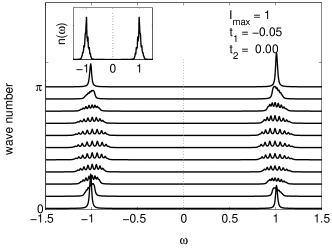
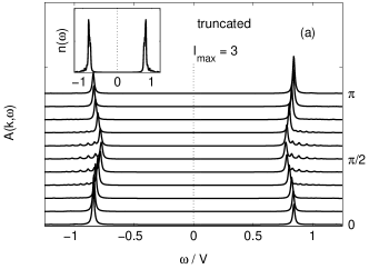
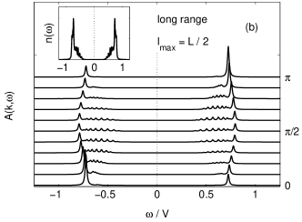
Figure 4: Spectral density $A(k,\omega)$ for spinless fermions for (a) truncated $V_{l}$ with $l_{max}=1$, (b) truncated $V_{l}$ with $l_{max}=13$ and (c) long-range $V_{l}$ with $t_{1}=-0.05V,t_{2}=0$. Insets show the density of states.

Interestingly, the relevant lowest excitations of the WL continue to be pairs of DWs in the case of the one-particle spectral density

$$\begin{split}A(k,\omega)&=\sum_{m}|\langle m^{+}|{c}^{\dagger}_{k,\uparrow}|\phi_{0}\rangle|^{2}\delta(\omega-(E^{+}_{m}-E_{0}))\\ &\quad+\sum_{m}|\langle m^{-}|{c}^{\phantom{\dagger}}_{k,\uparrow}|\phi_{0}\rangle|^{2}\delta(\omega-(E^{-}_{m}-E_{0}))\;,\end{split}$$ (3)

where $|m^{+}\rangle$ ($|m^{-}\rangle$) are eigenstates with eigenenergies $E^{+}_{m}$ ($E^{-}_{m}$) of the Hamiltonian with one particle added (removed). This observable is shown in Fig. 4 for a small NN hoping $t_{1}=-0.05V$ and three different cases for the interaction in (1): (i) NN repulsion only ($l_{\textrm{max}}=1$), where we see only a broad featureless continuum, (ii) slightly longer-range interaction with $l_{\textrm{max}}=3$, where we find a sharp quasiparticle below a continuum with small weight, and (iii) long-range Coulomb-repulsion with $l_{\textrm{max}}=L/2$, where the quasiparticle is observed above the continuum. We will now go on to show how these spectra - the continuum, the bound quasiparticle and the antibound quasiparticle - which have been obtained without any further assumption by exact diagonalization of the Hubbard-Wigner model, can be understood in terms of DWs and their interaction.

\psfrag{a}{(a)}\psfrag{b}{(b)}\psfrag{c}{(c)}\psfrag{t}{$t_{1}$}\includegraphics[width=173.44534pt]{ground_p1.eps}

Figure 5: (Color online) One of the two ground states (a) with circles denoting holes and solid arrows spinless fermions, pair of domain walls (indicated by dashed vertical lines) at distance $d=1$ created by adding one electron (b), configurations with distance $d=3$ between the DWs mediated by $t_{1}$(c).

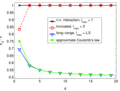
Figure 6: (Color online) Potential $E_{d}$ between two domain walls at distance $d$, see Fig. 5, for long-range electron-electron interaction ($l_{\textrm{max}}=L/2$, $\triangledown$), effective DW interaction (4) ($\ast$), and for truncated electron-electron interaction ($l_{\textrm{max}}=1$, $\times$ and $l_{\textrm{max}}=3$, $\circ$).

The schematic illustration in Fig. 5 shows that an additional electron again creates two DWs, this time both with an identical charge of $-e/2$. Again, their formal charge does not depend on details of the Hamiltonian: The total system has charge $-e$ (the additional electron) and both DWs are equivalent, which gives each DW a formal charge $-e/2$. The interaction $E_{d}$ between two domain walls at distance $d$ can be obtained by calculating the potential energy for a configuration where they are $d$ sites apart (as shown in Fig. 5 for distances $d=1,3$) by setting all hoppings to zero. The resulting interaction is depicted in Fig. 6 both for long-range and for truncated electron-electron interaction. If the Hamiltonian (1) has only NN Coulomb repulsion $l_{\textrm{max}}=1$, the energy ($\times$ in Fig. 6) does not depend on $d$, and the DWs are therefore independent. For $l_{\textrm{max}}=3$, the DWs are independent for large distance and attractive for small $d$. This means that their interaction has the opposite sign from the one expected from their formal charges of $-e/2$ each. For the long-range case $l_{\textrm{max}}=L/2$ ($\triangledown$ in Fig. 6), however, the asymptotic behavior of the interaction between two DWs decays like their inverse distance $d$:

$$E_{d}/V\sim 1/2+e^{2}/(4d)\;.$$ (4)

Hence, the interaction between the DWs is Coulomb-like and the prefactor is given by the two fractional charges of $-e/2$. The asymptotic relation ($\ast$ in Fig. 6) gives an excellent approximation already for rather small DW distances $d>1$. That (formal) fractional charges are the elementary excitations in charge ordered chains can be derived from the ground-state degeneracy alone, Hubbard78 without any reference to the particular form of the interaction stabilizing the degenerate ground states. In the case of long-range electron-electron interaction, and only in this case, the formal fractional charges have a very direct physical meaning: Their interaction corresponds exactly to that expected for ‘half-electrons’.

For the description of the photoemission process of a spinless fermion added to the perfect WL an effective low-energy Hamiltonian in terms of DWs can be obtained that contains hopping $t_{1}$ and the potential energy $E_{d}$. A reader interested in details for the following short derivation should consult Ref. Mayr06, , where an analogous treatment is given for the case depicted in Fig. 1. Starting from the ground state with $p=0$

$$|\phi_{\textrm{WL}}\rangle=\frac{1}{\sqrt{2}}(|0\uparrow 0\uparrow 0\uparrow\dots\rangle+|\uparrow 0\uparrow 0\uparrow 0\dots\rangle)$$ (5)

and adding an electron with momentum $k$, we arrive at a state $|\psi_{d=1,k}\rangle$ with momentum $k$ where the DW centers have distance $d=1$ (see Fig. 5(b))

$$\begin{split}|\psi_{d=1,k}\rangle&={c}^{\dagger}_{k,\uparrow}|\phi_{\textrm{WL}}\rangle=\frac{1}{\sqrt{L}}\sum_{r=1}^{L}\textrm{e}^{ikr}{c}^{\dagger}_{r,\uparrow}|\phi_{\textrm{WL}}\rangle=\\ &=\frac{1}{\sqrt{2L}}(\textrm{e}^{ik}|\uparrow\uparrow 0\uparrow 0\uparrow\dots\rangle-\textrm{e}^{2ikr}|\uparrow\uparrow\uparrow 0\uparrow 0\dots\rangle\\ &\quad\quad\quad-\textrm{e}^{3ik}|0\uparrow\uparrow\uparrow 0\uparrow\dots\rangle+\dots)\;,\end{split}$$ (6)

where the $-$ signs are due to a Fermi sign obtained by moving the creator through an existing electron. Once the two DWs have been created at distance $d=1$, they can move via NN electron hopping $t_{1}$:

$$\begin{split}T_{1}|\psi_{d=1,k}\rangle&=t_{1}\sum_{r=1}^{L}({c}^{\dagger}_{r,\uparrow}{c}^{\phantom{\dagger}}_{r+1,\uparrow}+\textrm{h.c.})\ |\psi_{d=1,k}\rangle=\\ &=\frac{t_{1}}{\sqrt{2L}}\left(\textrm{e}^{ik}(|\uparrow 0\uparrow\uparrow 0\uparrow\dots\rangle+|\uparrow\uparrow 0\uparrow\dots\uparrow\uparrow 0\rangle)\right.\\ &\quad-\textrm{e}^{2ikr}(|\uparrow\uparrow 0\uparrow\uparrow 0\dots\rangle+|0\uparrow\uparrow 0\uparrow 0\dots\uparrow\uparrow\rangle)\\ &\quad-\textrm{e}^{3ik}(|\uparrow 0\uparrow\uparrow 0\uparrow\dots\rangle+|0\uparrow\uparrow 0\uparrow\uparrow\dots\rangle)\\ &\left.\quad+\dots\right)=\\ &=2t_{1}\sin k|\psi_{d=3,k}\rangle\;,\end{split}$$ (7)

where $|\psi_{d=3,k}\rangle$ denotes the state with momentum $k$ and distance $d=3$ between the DWs (a complex phase has been absorbed into its definition). Repeating step (7), $d$ can grow further, which each $t_{1}$ process increasing (or reducing) $d$ in steps of two, see Fig. 5. (Additionally, $t_{1}$ can introduce more DWs, as in Fig. 1(b), but such processes cost energy and will be neglected in this low-energy analysis.)

We now arrive at the effective DW Hamiltonian $\mathcal{H}_{\textrm{DW}}$ in terms of $d$ and $k$.

$$\mathcal{H}_{\textrm{DW}}=\left(\begin{array}[]{cccccc}E_{1}&\tilde{t}_{1}(k)&0&\dots&&\\ \tilde{t}_{1}(k)&E_{3}&\tilde{t}_{1}(k)&0&\dots&\\ 0&\tilde{t}_{1}(k)&E_{5}&\tilde{t}_{1}(k)&0&\dots\\ \ \vdots&&&\ddots&&\end{array}\right)\;,$$ (8)

where the diagonal contains the potential energy $E_{d}$ and momentum $k$ enters the effective hopping $\tilde{t}_{1}(k)=2t_{1}\sin k$.

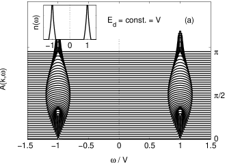
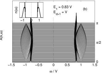
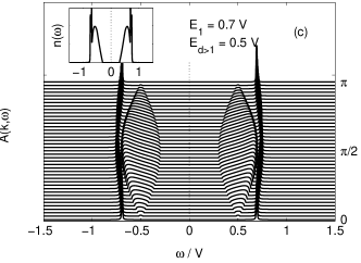
Figure 7: Spectral density obtained from the effective two-DW Hamiltonian (8) for $t_{1}=-0.05V,t_{2}=0$. (a) For non-interacting DWs with $E_{d}=\textrm{const}$, see Fig. 4 for the spectral density for the corresponding case $l_{\textrm{max}}=1$ in the electron Hamiltonian (1). (b) Attractive DW interaction with $E_{1}=0.83V,E_{d\geq 3}=V$, resulting from $l_{\textrm{max}}=3$ in (1), compare to Fig. 4. (c) Repulsive DW interaction with $E_{1}=0.7V,E_{d\geq 3}=0.5V$ as an approximation to the DW potential of the long-range electron Hamiltonian with $l_{\textrm{max}}=L/2$, the pertaining spectral density is seen in Fig. 4. The $\delta$ peaks of bound states have been slightly broadened and their height has been cut for better visibility of the 2 DW-continua.

We are interested in the spectral density (3), which can be written as

$$\begin{split}A(k,\omega)&=-\frac{1}{\pi}\Im\langle\phi_{0}|{c}^{\phantom{\dagger}}_{k,\uparrow}\frac{1}{\omega-(H-E_{0})+i0^{+}}{c}^{\dagger}_{k,\uparrow}|\phi_{0}\rangle\\ &\approx-\frac{1}{\pi}\Im\langle\psi_{1,k}|\frac{1}{\omega-\mathcal{H}_{\textrm{DW}}+i0^{+}}|\psi_{1,k}\rangle\;,\end{split}$$ (9)

i.e., we need the $(1,1)$ element of the inverse of the matrix $\omega-\mathcal{H}_{\textrm{DW}}$, which can be written as a continued fraction

$$(\omega-\mathcal{H}_{\textrm{DW}})^{-1}_{1,1}=\frac{1}{\omega-E_{1}-\frac{\tilde{t}_{1}(k)^{2}}{\omega-E_{3}-\frac{\tilde{t}_{1}(k)^{2}}{\omega-E_{5}-\dots}}}\,.$$ (10)

This fraction can be easily evaluated for the distance independent DW potential $E_{d}=V$ that is found, if only NN Coulomb repulsion is kept in the electronic Hamiltonian (1), see Fig. 6. We then obtain

$$A_{1}=(\omega-\mathcal{H}_{\textrm{DW}})^{-1}_{1,1}=\frac{\omega-\tilde{E}}{2\tilde{t}_{1}(k)^{2}}\pm\sqrt{\left(\frac{\omega-\tilde{E}}{2\tilde{t}_{1}(k)^{2}}\right)^{2}-\frac{1}{\tilde{t}_{1}(k)^{2}}}\,,$$ (11)

where $\tilde{E}$ is denotes the distance-independent DW potential, here $\tilde{E}=V$. The resulting spectral density has only a regular part and no singularities (except for $k=0,\pi$, where the hopping $\tilde{t}_{1}(k)$ vanishes), and is shown in Fig. 7. The incoherent two-DW continuum at energies $V-4t_{1}\sin k<\omega<V+4t_{1}\sin k$ results from the independent (since $E_{d}=\tilde{E}=\textrm{const}$) movement of the two DWs, and corresponds to the spectral density depicted in Fig. 4, which was calculated for the full fermionic model (1) with only NN repulsion ($l_{\textrm{max}}=1$).

Next, we move to the case $l_{\textrm{max}}=3$, which leads to a short range attraction between the DWs, see Fig. 6. Since the potential is constant for $d\geq 3$, we can use the result obtained above for $E_{d}=\textrm{const}$ in order to arrive at

$$A_{3}=\frac{1}{\omega-E_{1}-\tilde{t}_{1}(k)^{2}A_{1}}\,,$$ (12)

which is shown in Fig. 7. In addition to the continuum, we now find a pole where the denominator of (12) vanishes. It results from the DW attraction and corresponds to a bound quasiparticle with dispersion

$$\epsilon(k)=E_{1}+\frac{\tilde{t}_{1}(k)^{2}}{E_{1}-\tilde{E}}=E_{1}+\frac{(2t_{1}\sin k)^{2}}{E_{1}-\tilde{E}}\;,$$ (13)

where $\tilde{E}=V$ is the potential at distances $d\geq 3$ and $E_{1}\sim 0.83V$ the potential at $d=1$. For long-range electron-electron repulsion, we simplify the resulting DW potential to $E_{1}=0.7V,\tilde{E}=0.5V$ and can then apply (12) and (13). However, the quasiparticle is now an antibound state above the incoherent continuum, see Fig 7. This highly unusual situation is also observed in the spectra of the full model ( see Fig. 4) obtained by exact diagonalization. As we have seen here, it results from the DW repulsion and is thus a direct consequence of the long-range nature of the Coulomb repulsion absent from short-range models.

The only feature of the spectra for the full model (1) that is not reproduced in the simplified DW analysis is the transfer of spectral weight seen in Fig. 4 with more weight in photoemission (PES) at $k=0$ and more in inverse photoemission (IPES) at $k=\pi$. This transfer is caused by fluctuations around perfect charge order in the ground state induced by $t_{1}$, see Fig. 1, and will be discussed elsewhere.

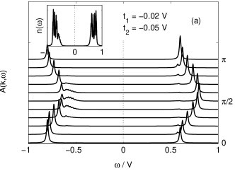
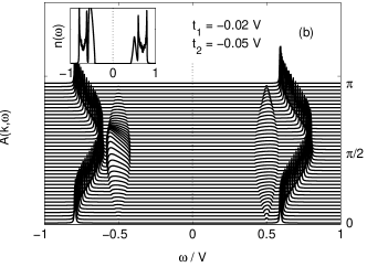
Figure 8: Spectral density $A(k,\omega)$ for $t_{1}=-0.02V,t_{2}=-0.05V$. (a) For the spinless-fermion Hamiltonian (1) with long-range interaction $l_{\textrm{max}}=L/2$ obtained by Lanczos diagonalization via (3). (b) For the effective DW-Hamiltonian (8) obtained by (12) with $E_{1}=0.7V+2t_{2}\cos 2k,\tilde{E}=0.5V$. Insets show the density of states.

Motivated by experimental data indicating that NNN hopping $t_{2}$ is larger than $t_{1}$ in Na₃Cu₂O₄, Horsch05 we now turn to the spectral density for $t_{2}\neq 0$. Via NNN hopping, an electron inserted into an empty site of the WL can hop over the occupied sites and move along the empty ones like a free fermion, and the same holds for a hole inserted into an occupied site. For $t_{1}=0$, we therefore obtain an independent-electron-like dispersion with $\epsilon(k)=V\ln 2+2t_{2}\cos 2k$ (not shown). The dispersion is the same in PES and IPES, which results in an indirect band gap with the highest occupied state at $k=\pi/2$ and the lowest unoccupied ones at $k=0,\pi$. Finite NN hopping $t_{1}\neq 0$ can be taken into account just like in the $t_{2}=0$ case discussed above by setting $E_{1}=V\ln 2+2t_{2}\cos 2k$ in (12). The resulting spectral density of the effective DW model is shown in Fig. 8 and the corresponding results for the fermion Hamiltonian (1) in Fig. 8. Both for PES and for IPES, we see the 2-DW continuum as well as a quasiparticle dispersion $\sim\cos 2k$. But we observe a certain particle-hole asymmetry: For IPES, the continuum has small weight and the width of the dispersion is $4t_{2}$ as for a free electron. For PES, the continuum is stronger and almost mixes with the quasiparticle at momenta $k\sim\pi/2$, which somewhat reduces the band width for the quasiparticle. We will see in the next section that the particle-hole asymmetry is strongly enhanced for electrons with spin.

IV Dynamics of electrons with spin

\psfrag{a}{(a)}\psfrag{b}{(b)}\psfrag{c}{(c)}\psfrag{d}{(d)}\psfrag{t}{$t_{1}$}\includegraphics[width=173.44534pt]{test_spin.eps}

Figure 9: (Color online) An electron added to the perfect WL, as Fig. 5, but for electrons with spin. In addition to the two DWs, an electron now creates a spinon (denoted by the unfilled circle/ellipse). As in the spinless case, the DWs can move via $t_{1}$, and the spinon can move via spin-flip processes.

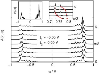
Figure 10: (Color online) Spectral density $A(k,\omega)$ with spin for $t_{1}=-0.05V,t_{2}=0$, $U=4V$, $L=16$. The right-hand inset shows a blow-up of IPES with a higher energy-resolution, the dashed and solid lines indicate spinon and ‘anti-holon’ branches (guides to the eye). The inset on the left shows the density of states.

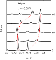
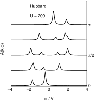
Figure 11: Comparison of the spectral density for Wigner and Hubbard models. (a) Blow-up with higher energy resolution of IPES for the Wigner model ($L=16$ sites) as in Fig. 10. The dashed and solid lines are guides to the eye indicating spinon and ‘anti-holon’ branches. (b) IPES for the half-filled 1D Hubbard model ($L=8$) with NN topping $t=1$ and $U=200t$.

Having understood the dynamics of the spinless system, i.e., of the charge sector, we now include the spin. An inserted electron or hole then produces a spinon in addition to the two DWs, see the cartoon in Fig. 9 illustrating the possible processes in the WL with spin. Again, the dynamics of the charge sector are determined by DW hopping via $t_{1}$. The spinon can move by spin-flip processes $\sim J_{2}=t_{2}^{2}/U$ or $\sim J_{1}=t_{1}^{2}/U$, a magnetic scale much smaller than the hopping scale. In this section, we will discuss how the spectral density indicates spin-charge separation similar as in the half-filled 1D Hubbard model.

Figure 12: (a) Charge-spin separation in 1D Hubbard model: Electron (solid line) decays into holon and spinon; (b) Wigner lattice at quarter-filling: Decay of electron into 2 DWs and a spinon; (c) Long-range Coulomb-repulsion of DWs generates a DW (anti) bound state (DWBS). This scattering state behaves like a holon.

At first, we will focus on NN hopping and compare the spectral density for $t_{1}=-0.05V,t_{2}=0$ with spin (Fig. 10) to the one without spin (Fig. 4). The 2-DW continuum is broader with spin, e.g. at $k=0$ and$k=\pi$, where the width of the continuum shrinks to zero in the spinless model. A more fundamental change is apparent in the antibound quasi-particle of the spinless case: It has evolved into a narrow structure with high spectral weight comprised of several peaks. Figure 11 shows a blow-up with higher energy resolution of this structure (in IPES) for $k=0$ to $k=\pi/2$. When we compare this blow-up to IPES for the usual half-filled 1D Hubbard model ($t=1,U=200t$) shown in Fig. 11, we observe remarkably similar structures. It is well known that an electron in the Hubbard model decays into a spinon and an anti-holon, see Fig. 12(a), and that IPES is given by a convolution of spinon and anti-holon branches. While this may not be so obvious on the present short 8-site ring, the anti-holon with width $\sim t$ and the spinon $\sim J=4t^{2}/U\ll t$ are clearly visible in the thermodynamic limit.Aichhorn03 The strong similarities seen in the spectral densities Fig. 11 for the Wigner and the Hubbard models let us conclude that the Wigner model likewise shows a convolution of spinon and anti-holon bands; the role of the anti-holon is now taken by the antibound 2-DW state that is the elementary collective excitation of the charge sector, see Fig. 12(c). Since the antibound 2-DW state already has a periodicity of $\pi$, see (13), the momentum range $k=0$ to $k=\pi/2$ corresponds to $k=0$ to $k=\pi$ in the Hubbard model with NN hopping, where the one-particle dispersion has periodicity $2\pi$. The width of the convolution is determined by that of the antibound 2-DW state, hence $\sim\frac{(2t_{1}\sin k)^{2}}{E_{1}-\tilde{E}}$, see (13); the spinon has almost no dispersion, because $\sim J_{1}\ll t_{1}$. The small differences between the Figs. 11 and 11 are due to weak interactions with the 2-DW continuum in the former case.

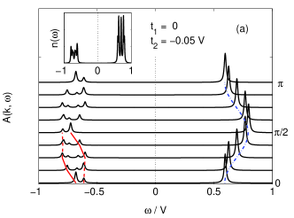
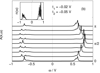
Figure 13: (Color online) Spectral density $A(k,\omega)$ with spin for (a) $t_{1}=0,t_{2}=-0.05V$, (b) $t_{1}=-0.02V,t_{2}=-0.05V$, $U=4V$, $L=16$. Insets on the left show the density of states. In (a), spinon and holon branches in PES are indicated by dashed and solid lines (guides to the eye), the dash-dotted line in IPES gives the one-particle dispersion $E(k)=V\ln 2+2t_{2}\cos 2k$.

We now turn to the spectral density for $t_{2}\neq 0$, at first choosing $t_{1}=0$ for simplicity. The ground state is then given by the perfectly charge ordered WL, an electron added in IPES goes into an empty site and can move freely on the empty sublattice, without any interaction with the occupied sublattice (as $t_{1}=0$). Consequently, IPES shows a one-particle-like tight-binding band with dispersion $E(k)=V\ln 2+2t_{2}\cos 2k$ just like in the spinless model, see $\omega>0$ in Fig. 13. The situation for a hole is, however, fundamentally different: The hole goes into the occupied sublattice, which is a half-filled Hubbard chain, and it therefore separates into spin and charge. The resulting spinon and holon branches in PES can be seen for $\omega<0$ in Fig. 13. (Again, the spectrum was found to agree to the one for the Hubbard model on eight sites. In this case even without any deviation, because there is no 2-DW continuum.) In this case of extreme particle-hole asymmetry, one and the same observable, the spectral density, shows both pure one-particle behavior (in the particle sector) and strongly correlated behavior (in the hole sector). If both $t_{2}$ and $t_{1}$ are active, the inserted particle (hole) can interact with the occupied (empty) sub-lattice, see the spectral density in Fig. 13. $t_{1}$-hopping processes now induce an additional incoherent 2-DW continuum, and we aquire incoherent weight in IPES. However, the strong particle-hole asymmetry persists: As in the spinless case shown in Fig. 8, we see that the quasiparticle in IPES remains largely intact and that - surprisingly - the peaks furthest from the Fermi energy remain sharpest.

V Summary and Conclusions

To conclude, we have investigated the dynamics of a quarter-filled Hubbard-Wigner model. Apart from being the most transparent situation on a Wigner lattice, quarter-filling is also appropriate for the edge-sharing chain compound Na₃Cu₂O₄. We find that electrons decay into a spinon and two domain walls as sketched in Fig. 12(b).

In the absence of the spinon, i.e., for the spinless model, we have investigated the effects of a truncated Coulomb interaction vs. fully long-range interaction in Sec. III. By comparing dynamic observables of the Wigner model (1) to those of an effective DW Hamiltonian, we have shown that the DWs and their interaction clearly manifest themselves in observables and are thus accessible to experiment. In the case of truly long-range electron-electron interaction, the formal fractional charges can be given a direct physical meaning that is consistent for both one-particle spectra $A(k,\omega)$ and two-particle dynamics $N(q,\omega)$. In models with truncated interaction, we still find formal fractional charges, but their interaction does no longer directly correspond to their formal charge. This difference has a strong impact on $A(k\omega)$: The DW repulsion due to long-range electron-electron interaction leads to a highly unusual anti-bound quasiparticle vs. a more conventional bound quasi-particle observed for truncated electron-electron interaction.

We have finally analyzed the Hubbard-Wigner model for electrons with spin, where we find the signatures of both charge fractionalization and spin-charge separation. Despite its composite nature, the antibound quasiparticle undergoes spin-charge separation reminiscent of an electron in the 1D Hubbard model, see Fig. 12(c). Experimentally, $t_{2}>t_{1}$ could be more relevant, Horsch05 and this case shows striking particle-hole asymmetry: For $t_{1}=0$, an added electron behaves like an independent particle while a hole shows strongly correlated behavior and decomposes into spinon and holon. Even for finite $t_{1}$, this behavior persists to some extend.

We thank A. M. Oleś, J. Unterhinninghofen and O. Gunnarsson for careful reading of the manuscript and for helpful suggestions.

References

- (1) S. Maekawa and T. Tohyama, Rep. Prog. Phys. 64, 383 (2001).
- (2) B. J. Kim et al., Nature Physics 2, 397 (2006).
- (3) M. Oshikawa and T. Senthil, Phys. Rev. Lett. 96, 060601 (2006).
- (4) R. B. Laughlin, Phys. Rev. Lett. 50, 1395 (1983).
- (5) A. J. Heeger, S. Kivelson, J. R. Schrieffer, and W. P. Su, Rev. Mod. Phys. 60, 781 (1988).
- (6) J. Hubbard, Phys. Rev. B 17, 494 (1978).
- (7) M. J. Rice and E. J. Mele, Phys. Rev. B 25, 1339 (1982).
- (8) A. Seidel and D.-H. Lee, Phys. Rev. Lett. 97, 056804 (2006).
- (9) E. Wigner, Phys. Rev. 46, 1002 (1934).
- (10) F. Nad and P. Monceau, J. Phys. Soc. Jpn. 75, 051005 (2006).
- (11) P. Horsch, M. Sofin, M. Mayr, and M. Jansen, Phys. Rev. Lett. 94, 076403 (2005).
- (12) M. Sofin, E.-M. Peters, and M. Jansen, J. Solid State Chem. 178, 3708 (2005).
- (13) K. Kudo et al., Phys. Rev. B 71, 104413 (2005).
- (14) R. Jackiw and C. Rebbi, Phys. Rev. D 13, 3398 (1976).
- (15) B. Valenzuela, S. Fratini, and D. Baeriswyl, Phys. Rev. B 68, 045112 (2003).
- (16) S. Fratini, B. Valenzuela, and D. Baeriswyl, Synthetic Metals 141, 194 (2004).
- (17) M. Mayr and P. Horsch, Phys. Rev. B 73, 195103 (2006).
- (18) As we treat rings with length , our interaction is in fact , with .
- (19) S. Capponi, D. Poilblanc, and T. Giamarchi, Phys. Rev. B 61, 13410 (2000).
- (20) M. Aichhorn, M. Daghofer, H. G. Evertz, and W. von der Linden, Phys. Rev. B 67, 161103(R) (2003).