Finite-Difference Time-Domain Study of Guided Modes in Nano-plasmonic Waveguides

Abstract

A conformal dispersive finite-difference time-domain (FDTD) method is developed for the study of one-dimensional (1-D) plasmonic waveguides formed by an array of periodic infinite-long silver cylinders at optical frequencies. The curved surfaces of circular and elliptical inclusions are modelled in orthogonal FDTD grid using effective permittivities (EPs) and the material frequency dispersion is taken into account using an auxiliary differential equation (ADE) method. The proposed FDTD method does not introduce numerical instability but it requires a fourth-order discretisation procedure. To the authors’ knowledge, it is the first time that the modelling of curved structures using a conformal scheme is combined with the dispersive FDTD method. The dispersion diagrams obtained using EPs and staircase approximations are compared with those from the frequency domain embedding method. It is shown that the dispersion diagram can be modified by adding additional elements or changing geometry of inclusions. Numerical simulations of plasmonic waveguides formed by seven elements show that row(s) of silver nanoscale cylinders can guide the propagation of light due to the coupling of surface plasmons.

I Introduction

It is well known that photonic crystals (PCs) offer unique opportunities to control the flow of light [1]. The basic idea is to design periodic dielectric structures that have a bandgap for a particular frequency range. Periodic dielectric rods with removed one or several rows of elements can be used as waveguiding devices when operating at bandgap frequencies. A lot of effort has been made to obtain a complete and wider bandgap. It has been shown that a triangular lattice of air holes in a dielectric background has a complete bandgap for TE (transverse electric) mode, while a square lattice of dielectric rods in air has a bandgap for TM (transverse magnetic) mode [2]. The devices operating in the bandgap frequencies are not the only option to guide the flow of light. Another waveguiding mechanism is the total internal reflection (TIR) in one-dimensional (1-D) periodic dielectric rods [3]. It is analysed in [3] that a single row of dielectric rods or air holes supports waveguiding modes and therefore can be also used as waveguide. In [4], the design of such waveguides consisting of several rows of dielectric rods with various spacings is proposed.

Recently, a new method for guiding electromagnetic waves in structures whose dimensions are below the diffraction limit has been proposed. The structures are termed as ‘plasmonic waveguides’ which have an operation of principle based on near-field interactions between closely spaced noble metal nanoparticles (spacing $\ll\lambda$) that can be efficiently excited at their surface plasmon frequency. The guiding principle relies on coupled plasmon modes set up by near-field dipole interactions that lead to coherent propagation of energy along the array. Analogous structures as waveguides in microwave regime include periodic metallic cylinders to support propagating waves [5], array of flat dipoles which support guided waves [6], and Yagi-Uda antennas [7, 8] etc. However, although these structures can be scaled to optical frequencies with appropriate material properties, their dimensions are limited by the so-called diffraction limit $\lambda/(2n)$. On the other hand, plasmonic waveguides employ the localisation of electromagnetic fields near metal surfaces to confine and guide light in regions much smaller than the free space wavelength and can effectively overcome the diffraction limit. Previous analysis of plasmonic structures includes the plasmon propagation along metal stripes, wires, or grooves in metal [9, 10, 11, 12, 13, 14], and the coupling between plasmons on metal particles in order to guide energy [15, 16] etc. Such subwavelength structures can also find their applications e.g. efficient absorbers and electrically small receiving antennas at microwave frequencies. Recently composite materials containing randomly distributed electrically conductive material and non-electrically conductive material have been designed [17]. They are noted to exhibit plasma-like responses at frequencies well below plasma frequencies of the bulk material.

The finite-difference time-domain (FDTD) method [18] is seen as the most popular numerical technique especially because of its flexibility in handling material dispersion as well as arbitrary shaped inclusions. In [19], the optical pulse propagation below the diffraction limit is shown using the FDTD method. Also with the FDTD method, the waveguide formed by several rows of silver nanorods arranged in hexagonal is studied [20]. Despite these examples of applying the FDTD method for the plasmonic structures, the accuracy of modelling has not been proven yet. When modelling curved structures, unless using extremely fine meshes, due to the nature of orthogonal and staggered grid of conventional FDTD, often modifications need to be applied in order to improve the numerical accuracy, such as the treatment of interfaces between different materials even for planar structures [21], and the improved conformal algorithms using structured meshes [22] for curved surfaces.

In addition to the modifications at material interfaces, the material frequency dispersion has also to be taken into account in FDTD modelling [23, 24, 25]. However, modelling dispersive materials with curved surfaces still remains to be a challenging topic due to the complexity in algorithm as well as the introduction of numerical instability. An alternative way to solve this problem is based on the idea of effective permittivities (EPs) [26, 27, 28] in the underlying Cartesian coordinate system, and the dispersive FDTD scheme can be therefore modified accordingly without affecting the stability of algorithm. In this paper, we first propose a novel conformal dispersive FDTD algorithm combining the EPs together with an auxiliary differential equation (ADE) method [18], then apply the developed method to the modelling of plasmonic waveguides formed by an array of circular or elliptical shaped silver cylinders at optical frequencies. Numerical FDTD simulation results are verified by a frequency domain embedding method [29]. To the authors’ knowledge, it is the first time that a conformal scheme is combined with the dispersive FDTD method for the modelling of nano-plasmonic waveguides.

II Conformal Dispersive FDTD Method Using Effective Permittivities

Conventionally, staircase approximations are often used to model curved electromagnetic structures in an orthogonal FDTD domain. Figure 1(a) shows an example layout of an infinite-long cylinder in the free space represented in a two-dimensional (2-D) orthogonal FDTD domain.

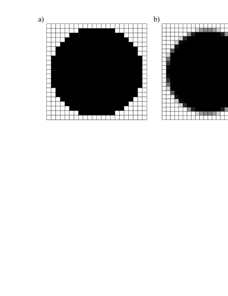
Figure 1: Comparison of the filling ratio for $E_{y}$ component in FDTD modelling of a circular cylinder using (a) staircase approximations and (b) a conformal scheme. The radius of circular cylinder is ten cells.

The approximated shape introduces spurious numerical resonant modes which do not exist in actual structures. On the other hand, using the concept of filling ratio, which is defined as the ratio of the area of material $\varepsilon_{2}$ to the area of a particular FDTD cell, the curvature can be properly represented in FDTD domain as shown in Fig. 1(b), where different levels of darkness indicate different filling ratios of material $\varepsilon_{2}$. The accuracy of modelling can be significantly improved compared with staircase approximations, as will be shown in a later section.

According to [28], the EP in a general form is given by

$$\varepsilon_{\rm{eff}}=\varepsilon_{\parallel}(1-n^{2})+\varepsilon_{\perp}n^{2},$$ (1)

where $n$ is the projection of the unit normal vector n along the field component as shown in Fig. 2,

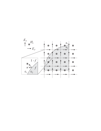
Figure 2: Layout of a quarter circular inclusion in orthogonal FDTD grid for $E_{y}$ component. The radius of circular cylinder is three cells.

$\varepsilon_{\parallel}$ and $\varepsilon_{\perp}$ are parallel and perpendicular permittivities to the material interface, respectively and defined as

$$\varepsilon_{\parallel} = f\varepsilon_{2}+(1-f)\varepsilon_{1},$$ (2)

$$\varepsilon_{\perp} = \left[f/\varepsilon_{2}+(1-f)/\varepsilon_{1}\right]^{-1},$$ (3)

where $f$ is the filling ratio of material $\varepsilon_{2}$ in a certain FDTD cell.

In this paper we consider the inclusions as silver cylinders, which at optical frequencies can be modelled using the Drude dispersion model

$$\varepsilon_{2}(\omega)=\varepsilon_{0}\left(1-\frac{\omega^{2}_{p}}{\omega^{2}-j\omega\gamma}\right),$$ (4)

where $\omega_{p}$ is the plasma frequency and $\gamma$ is the collision frequency. At the frequencies below the plasma frequency, the real part of permittivity is negative. In this paper, we assume that the silver cylinders are embedded in the free space ($\varepsilon_{1}=\varepsilon_{0}$).

In order to take into account the frequency dispersion of the material, the electric flux density D is introduced into standard FDTD updating equations. At each time step, D is updated directly from H and E can be calculated from D through the following steps. Substitute (2) and (3) into (1) and using the expressions for $\varepsilon_{1}$ and $\varepsilon_{2}$ (4), the constitutive relation in the frequency domain reads

$$\!\!\!\!\!\!\!\!\!\!\!\!\{\omega^{4}-2\gamma j\omega^{3}-[\gamma^{2}+(1-f)\omega^{2}_{p}]\omega^{2}+\gamma(1-f)\omega^{2}_{p}j\omega\}\textbf{D}$$

$$\!\!\!\!\!\!\!\!\!\!\!\!=[\omega^{4}-2\gamma j\omega^{3}-(\gamma^{2}+\omega^{2}_{p})\omega^{2}+\gamma\omega^{2}_{p}j\omega$$

$$\!\!\!\!+f(1-f)(1-n^{2})\omega^{4}_{p}]\varepsilon_{0}\textbf{E}.$$ (5)

Using the inverse Fourier transformation i.e. $j\omega\rightarrow\partial/\partial t$, we obtain the constitutive relation in the time domain as

$$\!\!\!\!\!\!\!\!\!\!\!\!\left\{\frac{\partial^{4}}{\partial t^{4}}+2\gamma\frac{\partial^{3}}{\partial t^{3}}+[\gamma^{2}+(1-f)\omega^{2}_{p}]\frac{\partial^{2}}{\partial t^{2}}+\gamma(1-f)\omega^{2}_{p}\frac{\partial}{\partial t}\right\}\textbf{D}$$

$$\!\!\!\!\!\!\!\!\!\!\!\!=\bigg{[}\frac{\partial^{4}}{\partial t^{4}}+2\gamma\frac{\partial^{3}}{\partial t^{3}}+(\gamma^{2}+\omega^{2}_{p})\frac{\partial^{2}}{\partial t^{2}}+\gamma\omega^{2}_{p}\frac{\partial}{\partial t}$$

$$\!\!\!\!+f(1-f)(1-n^{2})\omega^{4}_{p}\bigg{]}\varepsilon_{0}\textbf{E}.$$ (6)

The FDTD simulation domain is represented by an equally spaced three-dimensional (3-D) grid with periods $\Delta x$, $\Delta y$ and $\Delta z$ along $x$-, $y$- and $z$-directions, respectively. The time step is $\Delta t$. For discretisation of (6), we use the central finite difference operators in time ($\delta_{t}$) and the central average operator with respect to time ($\mu_{t}$):

$$\!\!\!\!\!\!\!\!\!\frac{\partial^{4}}{\partial t^{4}}\rightarrow\frac{\delta^{4}_{t}}{(\Delta t)^{4}},~{}~{}~{}\frac{\partial^{3}}{\partial t^{3}}\rightarrow\frac{\delta^{3}_{t}}{(\Delta t)^{3}}\mu_{t},~{}~{}~{}\frac{\partial^{2}}{\partial t^{2}}\rightarrow\frac{\delta^{2}_{t}}{(\Delta t)^{2}}\mu^{2}_{t},$$

$$\!\!\!\!\!\!\!\!\!\frac{\partial}{\partial t}\rightarrow\frac{\delta_{t}}{\Delta t}\mu^{3}_{t},~{}~{}~{}1\rightarrow\mu^{4}_{t},$$ (7)

where the operators $\delta_{t}$ and $\mu_{t}$ are defined as in [30]:

$$\delta_{t}\textbf{F}|^{n}_{m_{x},m_{y},m_{z}} \equiv \textbf{F}|^{n+\frac{1}{2}}_{m_{x},m_{y},m_{z}}-\textbf{F}|^{n-\frac{1}{2}}_{m_{x},m_{y},m_{z}},$$ (8)

$$\mu_{t}\textbf{F}|^{n}_{m_{x},m_{y},m_{z}} \equiv \frac{\textbf{F}|^{n+\frac{1}{2}}_{m_{x},m_{y},m_{z}}+\textbf{F}|^{n-\frac{1}{2}}_{m_{x},m_{y},m_{z}}}{2}.$$ (9)

Here F represents field components and $m_{x},m_{y},m_{z}$ are indices corresponding to a certain discretisation point in the FDTD domain. The discretised Eq. (6) reads

$$\!\!\!\!\!\!\!\!\!\!\!\!\bigg{\{}\frac{\delta^{4}_{t}}{(\Delta t)^{4}}+2\gamma\frac{\delta^{3}_{t}}{(\Delta t)^{3}}\mu_{t}+\left[\gamma^{2}+(1-f)\omega^{2}_{p}\right]\frac{\delta^{2}_{t}}{(\Delta t)^{2}}\mu^{2}_{t}$$

$$\!\!\!\!\!\!\!+\gamma(1-f)\omega^{2}_{p}\frac{\delta_{t}}{\Delta t}\mu^{3}_{t}\bigg{\}}\textbf{D}=\bigg{[}\frac{\delta^{4}_{t}}{(\Delta t)^{4}}+2\gamma\frac{\delta^{3}_{t}}{(\Delta t)^{3}}\mu_{t}$$

$$\!\!\!\!\!\!\!+(\gamma^{2}+\omega^{2}_{p})\frac{\delta^{2}_{t}}{(\Delta t)^{2}}\mu^{2}_{t}+\gamma\omega^{2}_{p}\frac{\delta_{t}}{\Delta t}\mu^{3}_{t}$$

$$\!\!\!\!\!\!\!+f(1-f)(1-n^{2})\omega^{4}_{p}\mu^{4}_{t}\bigg{]}\varepsilon_{0}\textbf{E}.$$ (10)

Note that in the above equations we have kept all terms to be the fourth-order to guarantee numerical stability. Equation (10) can be written as

$$\!\!\!\frac{\textbf{D}^{n+1}-4\textbf{D}^{n}+6\textbf{D}^{n-1}-4\textbf{D}^{n-2}+\textbf{D}^{n-3}}{(\Delta t)^{4}}$$

$$~{}+\gamma\frac{\textbf{D}^{n+1}-2\textbf{D}^{n}+2\textbf{D}^{n-2}-\textbf{D}^{n-3}}{(\Delta t)^{3}}$$

$$~{}+\left[\gamma^{2}+(1-f)\omega^{2}_{p}\right]\frac{\textbf{D}^{n+1}-2\textbf{D}^{n-1}+\textbf{D}^{n-3}}{4(\Delta t)^{2}}$$

$$~{}+\gamma(1-f)\omega^{2}_{p}\frac{\textbf{D}^{n+1}+2\textbf{D}^{n}-2\textbf{D}^{n-2}-\textbf{D}^{n-3}}{8\Delta t}$$

$$\!\!\!=\varepsilon_{0}\frac{\textbf{E}^{n+1}-4\textbf{E}^{n}+6\textbf{E}^{n-1}-4\textbf{E}^{n-2}+\textbf{E}^{n-3}}{(\Delta t)^{4}}$$

$$~{}+\varepsilon_{0}\gamma\frac{\textbf{E}^{n+1}-2\textbf{E}^{n}+2\textbf{E}^{n-2}-\textbf{E}^{n-3}}{(\Delta t)^{3}}$$

$$~{}+\varepsilon_{0}\left(\gamma^{2}+\omega^{2}_{p}\right)\frac{\textbf{E}^{n+1}-2\textbf{E}^{n-1}+\textbf{E}^{n-3}}{4(\Delta t)^{2}}$$

$$~{}+\varepsilon_{0}\gamma\omega^{2}_{p}\frac{\textbf{E}^{n+1}+2\textbf{E}^{n}-2\textbf{E}^{n-2}-\textbf{E}^{n-3}}{8\Delta t}$$

$$~{}+\frac{\varepsilon_{0}f(1-f)(1-n^{2})\omega^{4}_{p}}{16}\big{(}\textbf{E}^{n+1}+4\textbf{E}^{n}+6\textbf{E}^{n-1}$$

$$~{}~{}~{}~{}+4\textbf{E}^{n-2}+\textbf{E}^{n-3}\big{)}.$$ (11)

The indices $m_{x}$, $m_{y}$ and $m_{z}$ are omitted from (11) since E and D are located at same locations. Solving for $\textbf{E}^{n+1}$ then the updating equation for E in FDTD iterations reads

$$\!\!\!\!\!\!\!\!\!\!\!\!\!\!\!\!\!\!\!\textbf{E}^{n+1}=[b_{0}\textbf{D}^{n+1}+b_{1}\textbf{D}^{n}+b_{2}\textbf{D}^{n-1}+b_{3}\textbf{D}^{n-2}+b_{4}\textbf{D}^{n-3}$$

$$~{}-(a_{1}\textbf{E}^{n}+a_{2}\textbf{E}^{n-1}+a_{3}\textbf{E}^{n-2}+a_{4}\textbf{E}^{n-3})]/a_{0},$$ (12)

with the coefficients given by

$$a_{0}\!\!\!\! = \!\!\!\!\varepsilon_{0}\Bigg{[}\frac{1}{(\Delta t)^{4}}+\frac{\gamma}{(\Delta t)^{3}}+\frac{\gamma^{2}+\omega^{2}_{p}}{4(\Delta t)^{2}}+\frac{\gamma\omega^{2}_{p}}{8\Delta t}$$

$$~{}~{}~{}~{}+\frac{f(1-f)(1-n^{2})\omega^{4}_{p}}{16}\Bigg{]},$$

$$a_{1}\!\!\!\! = \!\!\!\!\varepsilon_{0}\left[-\frac{4}{(\Delta t)^{4}}-\frac{2\gamma}{(\Delta t)^{3}}+\frac{\gamma\omega^{2}_{p}}{4\Delta t}+\frac{f(1-f)(1-n^{2})\omega^{4}_{p}}{4}\right],$$

$$a_{2}\!\!\!\! = \!\!\!\!\varepsilon_{0}\left[\frac{6}{(\Delta t)^{4}}-\frac{\gamma^{2}+\omega^{2}_{p}}{2(\Delta t)^{2}}+\frac{3f(1-f)(1-n^{2})\omega^{4}_{p}}{8}\right],$$

$$a_{3}\!\!\!\! = \!\!\!\!\varepsilon_{0}\left[-\frac{4}{(\Delta t)^{4}}+\frac{2\gamma}{(\Delta t)^{3}}-\frac{\gamma\omega^{2}_{p}}{4\Delta t}+\frac{f(1-f)(1-n^{2})\omega^{4}_{p}}{4}\right],$$

$$a_{4}\!\!\!\! = \!\!\!\!\varepsilon_{0}\Bigg{[}\frac{1}{(\Delta t)^{4}}-\frac{\gamma}{(\Delta t)^{3}}+\frac{\gamma^{2}+\omega^{2}_{p}}{4(\Delta t)^{2}}-\frac{\gamma\omega^{2}_{p}}{8\Delta t}$$

$$~{}~{}~{}~{}+\frac{f(1-f)(1-n^{2})\omega^{4}_{p}}{16}\Bigg{]},$$

$$b_{0}\!\!\!\! = \!\!\!\!\frac{1}{(\Delta t)^{4}}+\frac{\gamma}{(\Delta t)^{3}}+\frac{\gamma^{2}+(1-f)\omega^{2}_{p}}{4(\Delta t)^{2}}+\frac{\gamma(1-f)\omega^{2}_{p}}{8\Delta t},$$

$$b_{1}\!\!\!\! = \!\!\!\!-\frac{4}{(\Delta t)^{4}}-\frac{2\gamma}{(\Delta t)^{3}}+\frac{\gamma(1-f)\omega^{2}_{p}}{4\Delta t},$$

$$b_{2}\!\!\!\! = \!\!\!\!\frac{6}{(\Delta t)^{4}}-\frac{\gamma^{2}+(1-f)\omega^{2}_{p}}{2(\Delta t)^{2}},$$

$$b_{3}\!\!\!\! = \!\!\!\!-\frac{4}{(\Delta t)^{4}}+\frac{2\gamma}{(\Delta t)^{3}}-\frac{\gamma(1-f)\omega^{2}_{p}}{4\Delta t},$$

$$b_{4}\!\!\!\! = \!\!\!\!\frac{1}{(\Delta t)^{4}}-\frac{\gamma}{(\Delta t)^{3}}+\frac{\gamma^{2}+(1-f)\omega^{2}_{p}}{4(\Delta t)^{2}}-\frac{\gamma(1-f)\omega^{2}_{p}}{8\Delta t},$$

The computations of H and D are performed using Yee’s standard updating equations in the free space. Note that if the plasma frequency is equal to zero ($\omega_{p}=0$), then (12) reduces to the updating equation in the free space i.e. $\textbf{E}=\textbf{D}/\varepsilon_{0}$.

III FDTD Calculation of Dispersion Diagram

Applying the Bloch’s periodic boundary conditions (PBCs) [31, 32, 33, 34, 35, 36], FDTD method can be used to model periodic structures and calculate their dispersion diagrams [37, 38]. For any periodic structures, the field at any time should satisfy the Bloch theory, i.e.

$$\textbf{E}(\textbf{d}+\textbf{a})=\textbf{E}(\textbf{d})e^{j\bf{ka}},~{}~{}~{}\textbf{H}(\textbf{d}+\textbf{a})=\textbf{H}(\textbf{d})e^{j\bf{ka}},$$ (13)

where d is the distance vector of any location in the computation domain, k is the wave vector and a is the lattice vector along the direction of periodicity. When updating the fields at the boundary of the computation domain using FDTD, the required fields outside the computation domain can be calculated using known field values inside the domain through Eq. (13). Although instead of using real values in conventional FDTD computations, the calculation of dispersion diagrams requires complex field values, since only one unit cell is modelled, the computation load is not significantly increased.

First we apply the developed conformal dispersive FDTD method to calculate the dispersion diagram for 1-D plasmonic waveguides formed by an array of periodic infinite-long (along $z$-direction) circular silver cylinders. As shown in Fig. 3, the 2-D simulation domain ($x$-$y$) with TE modes (therefore only $E_{x}$, $E_{y}$ and $H_{z}$ are non-zero fields) is truncated using Bloch’s PBCs in $x$-direction and Berenger’s perfectly matched layers (PMLs) [39] in $y$-direction.

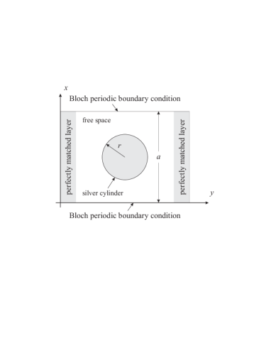
Figure 3: The layout of the 2-D FDTD computation domain for calculating dispersion diagram for 1-D periodic structures. The inclusion has a circular cross-section with radius $r$ and the period of the 1-D infinite structure is $a$.

The Berenger’s PMLs have excellent performance for absorbing propagating waves [39], however for evanescent waves, field shows growing behaviour inside PMLs. Since the waves radiated by point or line sources consist of both propagating and evanescent components, extra space (typically a quarter wavelength at the frequency of interest) between PMLs and the circular inclusion is added to allow the evanescent waves to decay before reaching the PMLs.

The radius of silver cylinders is $r=2.5\times 10^{-8}$ m and the period is $a=7.5\times 10^{-8}$ m. The plasma and collision frequencies are $\omega_{p}=9.39\times 10^{15}$ rad/s and $\gamma=3.14\times 10^{13}$ Hz, respectively in order to closely match the bulk dielectric function of silver [40]. The FDTD cell size is $\Delta x=\Delta y=2.5\times 10^{-9}$ m with the time step $\Delta t=\Delta x/(\sqrt{2}c)$ s (where $c$ is the speed of light in the free space) according to the Courant stability criterion [18]. Although the stability condition for high-order FDTD method is typically more strict than the conventional one, since the average operator $\mu_{t}$ is applied to develop the algorithm, we have not found any instability for a complete time period of more than 40,000 time steps used in all simulations.

A wideband magnetic line source is placed at an arbitrary location in the free space region of the 2-D simulation domain in order to excite all resonant modes of the structure within the frequency range of interest (normalised frequency $\overline{f}=\omega a/(2\pi c)\in[0\sim 0.5]$):

$$g(t)=e^{-\left(\frac{t-t_{0}}{\tau}\right)^{2}}\cdot e^{j\omega t}$$ (14)

where $t_{0}$ is the initial time delay, $\tau$ defines the pulse width and $\omega$ is the centre frequency of the pulse ($\overline{f}=0.25$). The magnetic fields at one hundred random locations in the free space region are recorded during simulations, transformed into the frequency domain and combined to extract individual resonant mode corresponding to each local maximum. For each wave vector, a total number of 40,000 time steps are used in our simulations to obtain enough accurate frequency domain results.

In order to demonstrate the advantage of EPs and validate the proposed conformal dispersive FDTD method, we have also performed simulations using staircase approximations for the circular cylinder, as shown in Fig. 1(a). Figure 4 shows the comparison of the first resonant frequency (transverse mode) at wave vector $k_{x}=\pi/a$ of the plasmonic waveguide calculated using the FDTD method with staircase approximations, the FDTD method with EPs and the frequency domain embedding method [41].

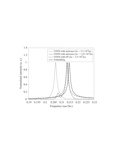
Figure 4: Comparison of the first resonant frequency (transverse mode) at wave vector $k_{x}=\pi/a$ calculated using the FDTD method with staircase approximations, the FDTD method with EPs and the frequency domain embedding method.

With the same FDTD spatial resolutions, the model using EP shows excellent agreement with the results from the frequency domain embedding method, on the contrary, the staircase approximation not only leads to a shift of the main resonant frequency, but also introduces a spurious numerical resonant mode which does not exist in actual structures. The same effect has also been found for non-dispersive dielectric cylinders [42]. It is also shown in Fig. 4 that although one may correct the main resonant frequency using finer meshes, the spurious resonant mode still remains.

The problem of frequency shift and spurious modes become severer when calculating higher guided modes near the ‘flat band’ region (i.e the region where waves travel at a very low phase velocity). Even with a refined spatial resolution, the staircase approximation fails to provide correct results (not shown). On the other hand, using the proposed conformal dispersive FDTD scheme, all resonant modes are correctly captured in FDTD simulations as demonstrated by the comparison with the embedding method as shown in Fig. 5.

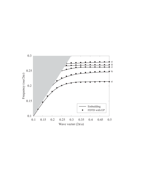
Figure 5: Comparison of dispersion diagrams for an array of infinite-long (along $z$-direction) circular silver cylinders calculated using the FDTD method with EPs and the frequency domain embedding method.

According to previous analysis using the frequency embedding method, the fundamental mode in the modelled plasmonic waveguide is transverse mode and the second guided mode is longitudinal [41], which is also shown by the distribution of electric field intensities in Fig. 6 from our FDTD simulations.

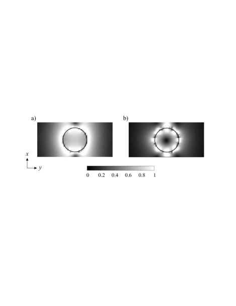
Figure 6: Normalised total electric field intensities corresponding to (a) transverse and (b) longitudinal modes [41] at wave number $k_{x}=\pi/a$ as marked in Fig. 5. The structure is infinite along $x$-direction.

The higher guided modes are referred to as plasmon modes. For demonstration of field symmetries and due to the TE mode considered in our simulations, we have plotted the distributions of magnetic field corresponding to different resonant modes at wave number $k_{x}=\pi/a$ as marked in Fig. 5, as shown in Fig. 7.

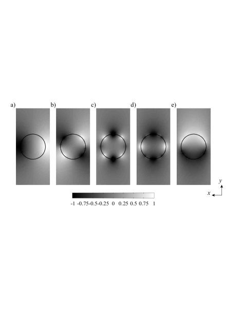
Figure 7: Normalised distributions of magnetic field corresponding to different resonant modes at wave number $k_{x}=\pi/a$ as marked in Fig. 5: (a), (c), (d): even modes, and (b), (e): odd modes. The structure is infinite along $x$-direction. (Note that the coordinate has been rotated 90 degrees anti-clockwise from Fig. 3 for better presentation of the figure.)

Sinusoidal sources for excitation of certain single mode are used and the sources are placed at different locations corresponding to different symmetries of field patterns. All field patterns are plotted after the steady state is reached in simulations. The modes (a), (c) and (d) in Fig. 7 are even modes (relative to the direction of periodicity of the waveguide i.e. $x$-axis), and (b) and (e) are considered as odd modes.

The above comparison of the simulation results calculated using the conformal dispersive FDTD method and the embedding method clearly demonstrates the effectiveness of applying the EPs in FDTD modelling. Furthermore, in contrast to the embedding method, the main advantage of the FDTD method is that arbitrary shaped geometries can be easily modelled. We have applied the conformal dispersive FDTD method to study the effect of different inclusions on the dispersion diagrams of 1-D plasmonic waveguides. The geometries considered are two rows of periodic infinite-long (along $z$-direction) circular silver cylinders arranged in square lattice and a single row of periodic infinite-long (along $z$-direction) elliptical silver cylinders. The elliptical element has a ratio of semimajor-to-semiminor axis 2:1, where the semiminor axis is equal to the radius of the circular element ($25.0$ nm). For the two rows of circular nanorods, the spacing between two rows (centre-to-centre distance) is $75.0$ nm. The dispersion diagrams for these structures are plotted in Figs. 8 and 10.

Figure 8: Dispersion diagram for two rows of periodic infinite-long (along $z$-direction) circular silver cylinders arranged in square lattice calculated from conformal dispersive FDTD simulations.

Comparing the dispersion diagrams for a single circular element in Fig. 5 and two circular elements in Fig. 8 we can see that the dispersion diagram has been modified due to the change of inclusion. The strong coupling between two elements introduces additional guided modes to appear in dispersion diagram. Such phenomenon has also been studied for dielectric (non-dispersive) nanorods previously [4]. The distributions of magnetic field for selected guided modes as marked in Fig. 8 are plotted in Fig. 9.

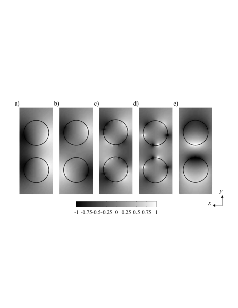
Figure 9: Normalised distributions of magnetic field corresponding to different guided modes as marked in Fig. 8: (a), (c), (d): even modes, and (b), (e): odd modes. The structure is infinite along $x$-direction. (Note that the coordinate has been rotated 90 degrees anti-clockwise from Fig. 3 for better presentation of the figure.)

The modes (a), (c) and (d) are even modes while (b) and (e) are odd modes.

The dispersion diagram for a single elliptical element as inclusion is shown in Fig. 10.

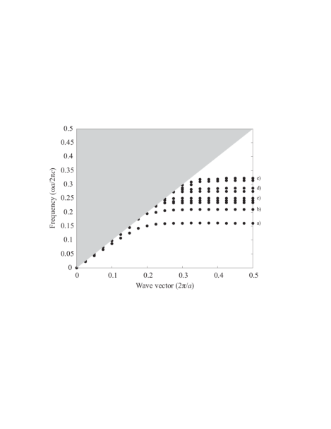
Figure 10: Dispersion diagram for a single row of periodic infinite-long (along $z$-direction) elliptical silver cylinders calculated from conformal dispersive FDTD simulations.

It can be seen that more guided modes appear which is caused by the change of inclusion’s geometrical shape from circular to elliptical. The frequency corresponding to the lowest mode has been lowered due to the increase of inclusion’s volume. The distributions of magnetic field for selected guided modes are plotted in Fig. 11.

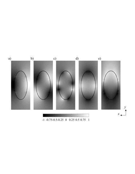
Figure 11: Normalised distributions of magnetic field corresponding to different guided modes as marked in Fig. 10: (a), (d): even modes, and (b), (c), (e): odd modes. The structure is infinite along $x$-direction. (Note that the coordinate has been rotated 90 degrees anti-clockwise from Fig. 3 for better presentation of the figure.)

The modes (a) and (d) are even modes and (b), (c) and (e) are odd modes, respectively.

IV Wave Propagation in Plasmonic Waveguides formed by Finite Number of Elements

In order to study wave propagations in plasmonic waveguides formed by a finite number of silver nanorods, we have replaced PBCs in $x$-direction with PMLs and added additional cells for the free space region to the simulation domain. The number of nanorods under study is seven. The spacing (pseudo-period) between adjacent elements remains the same as for infinite structures considered in the previous section. For a single mode excitation, we choose the frequency of corresponding mode from dispersion diagram, and excite sinusoidal sources at different locations with respect to the symmetry of different guided modes at one end of the waveguides.

For the plasmonic waveguides formed by different types of inclusions, we have chosen certain eigen modes: mode Fig. 7(a) for a single row of circular cylinders, mode Fig. 9(d) for two rows of circular cylinders, and mode Fig. 11(e) for a single row of elliptical cylinders. The distributions of magnetic field intensity for different waveguides operating in these guided modes are plotted in Fig. 12.

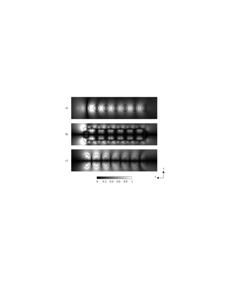
Figure 12: Normalised distributions of magnetic field intensity corresponding to different guided modes for seven-element plasmonic waveguides formed by (a) a single row of circular nanorods (the corresponding eigen mode is shown in Fig. 7(a)) (b) two rows of circular nanorods arranged in square lattice (the corresponding eigen mode is shown in Fig. 9(c)) (c) a single row of elliptical nanorods (the corresponding eigen mode is shown in Fig. 11(e)). (Note that the coordinate has been rotated 90 degrees anti-clockwise from Fig. 3 for better presentation of the figure.)

The field plots are taken after the steady state is reached in simulations. It is clearly seen that single guided modes are coupled into these waveguides but the excitation of certain modes highly depends on the symmetry of field patterns. The energy that can be coupled into the waveguides also depends on the matching between source and the plasmonic waveguide.

V Conclusions

In conclusion, we have developed a conformal dispersive FDTD method for the modelling of plasmonic waveguides formed by an array of periodic infinite-long silver cylinders at optical frequencies. The conformal scheme is based on effective permittivities and its main advantage is that since conventional orthogonal FDTD grid is maintained in simulations, no numerical instability is introduced. The material frequency dispersion is taken into account using an auxiliary differential equation method. The comparison of dispersion diagrams for one-dimensional periodic silver cylinders calculated using the conformal dispersive FDTD method, the conventional dispersive FDTD method with staircase approximations and the frequency domain embedding method demonstrates the accuracy of the proposed method. It is shown that by adding additional element or changing the geometry of inclusions, the corresponding dispersion diagram can be modified. Numerical simulations of plasmonic waveguides formed by seven elements show that the eigen modes in infinite structures can be excited but highly depend on the symmetry of field patterns of certain modes. Further work includes the investigation of the effects of different number of elements in plasmonic waveguides on guided modes, and the calculation of group velocity of different modes propagating in these waveguides. Although results presented in this paper have been focused at optical frequencies, with future advances in microwave plasmonic materials, novel applications can be found in the designs of small antenna and efficient absorbers.

References

- [1] J. D. Joannopoulos, R. D. Meade, and J. N. Winn, Photonic crystals: Molding the flow of light, Princeton U. Press, Princeton, N.J., 1995.
- [2] G. Qiu, F. Lin, and Y. Li, “Complete two-dimensional bandgap of photonic crystals of a rectangular Bravais lattice,” Opt. Commun., vol. 219, pp. 285-288, 2003.
- [3] S. Fan, J. Winn, A. Devenyi, J. C. Chen, R. D. Meade, and J. D. Joannopoulos, “Guided and defect modes in periodic dielectric waveguides,” J. Opt. Soc. Am. B, vol. 12, pp. 1267-1272, 1995.
- [4] D. Chigrin, A. Lavrinenko, and C. Sotomayor Torres, “Nanopillars photonic crystal waveguides,” Opt. Express, vol. 12, pp. 617-622, 2004.
- [5] J. Shefer, “Periodic cylinder arrays as transmission lines,” IEEE Trans. Microwave Theory Tech., vol. 11, pp. 55-61, Jan. 1963.
- [6] B. A. Munk, D. S. Janning, J. B. Pryor, and R. J. Marhefka, “Scattering from surface waves on finite FSS,” IEEE Trans. Antennas Propagat., vol. 49, pp. 1782-1793, Dec. 2001.
- [7] R. J. Mailloux, “Antenna and wave theories of infinite Yagi-Uda arrays,” IEEE Trans. Antennas Propagat., vol. 13, pp. 499-506, Jul. 1965.
- [8] A. D. Yaghjian, “Scattering-matrix analysis of linear periodic arrays,” IEEE Trans. Antennas Propagat., vol. 50, pp. 1050-1064, Aug. 2002.
- [9] J. C. Weeber, A. Dereux, C. Girard, J. R. Krenn and J. P. Goudonnet, “Plasmon polaritons of metallic nanowires for controlling submicron propagation of light,” Phys. Rev. B, vol. 60, pp. 9061-9068, 1999.
- [10] B. Lamprecht, J. R. Krenn, G. Schider, H. Ditlbacher, M. Salerno, N. Felidj, A. Leitner, F. R. Aussenegg, and J. C. Weeber, “Surface plasmon propagation in microscale metal stripes,” Appl. Phys. Lett., vol. 79, pp. 51-53, 2001.
- [11] T. Yatsui, M. Kourogi, and M. Ohtsu , “Plasmon waveguide for optical far/near-field conversion,” Appl. Phys. Lett., vol. 79, pp. 4583-4585, 2001.
- [12] R. Zia, M. D. Selker, P. B. Catrysse, and M. L. Brongersma, “Geometries and materials for subwavelength surface plasmon modes,” J. Opt. Soc. Am. A, vol. 21, pp. 2442-2446, 2004.
- [13] R. Charbonneau, N. Lahoud, G. Mattiussi, and P. Berini, “Demonstration of integrated optics elements based on long-ranging surface plasmon polaritons,” Opt. Express, vol. 13, pp. 977-984, 2005.
- [14] D. F. P. Pile, D. K. Gramotnev, “Channel plasmon-polariton in a triangular groove on a metal surface,” Opt. Lett., vol. 29, pp. 1069-1071, 2004.
- [15] M. Quinten, A. Leitner, J. R. Krenn, and F. R. Aussenegg, “Electromagnetic energy transport via linear chains of silver nanoparticles,” Opt. Lett., vol. 23, pp. 1331-1333, 1998.
- [16] M. L. Brongersma, J. W. Hartman, and H. A. Atwater, “Electromagnetic energy transfer and switching in nanoparticle chain arrays below the diffraction limit,” Phys. Rev. B, vol. 62, pp. 16356-16359, 2000.
- [17] T. J. Shepherd, C. R. Brewitt-Taylor, P. Dimond, G. Fixter, A. Laight, P. Lederer, P. J. Roberts, P. R. Tapster, and I. J. Youngs, “3D microwave photonic crystals: Novel fabrication and structures,” Electron. Lett., vol. 34, pp. 787-789, 1998.
- [18] A. Taflove, Computational Electrodynamics: The Finite Difference Time Domain Method. Norwood, MA: Artech House, 1995.
- [19] S. A. Maier, P. G. Kik, and H. A. Atwater, “Optical pulse propagation in metal nanoparticle chain waveguides,” Phys. Rev. B, vol. 67, pp. 205402, 2003.
- [20] W. M. Saj, “FDTD simulations of 2D plasmon waveguide on silver nanorods in hexagonal lattice,” Opt. Express, vol. 13, no. 13, pp. 4818-4827, June 2005.
- [21] K.-P. Hwang, and A. C. Cangellaris, “Effective permittivities for second-order accurate FDTD equations at dielectric interfaces,” IEEE Microwave Wirel. Compon. Lett., vol. 11, pp. 158-160, 2001.
- [22] Y. Hao, and C. J. Railton, “Analyzing electromagnetic structures with curved boundaries on Cartesian FDTD meshes,” IEEE Trans. Microwave Theory Tech., vol. 46, pp. 82-88, Jan. 1998.
- [23] R. Luebbers, F. P. Hunsberger, K. Kunz, R. Standler, and M. Schneider, “A frequency-dependent finite-difference time-domain formulation for dispersive materials”, IEEE Trans. Electromagn. Compat., vol. 32, pp. 222-227, Aug. 1990.
- [24] O. P. Gandhi, B.-Q. Gao, and J.-Y. Chen, “A frequency-dependent finite-difference time-domain formulation for general dispersive media,” IEEE Trans. Microwave Theory Tech., vol. 41, pp. 658-664, Apr. 1993.
- [25] D. M. Sullivan, “Frequency-dependent FDTD methods using Z transforms,” IEEE Trans. Antennas Propagat., vol. 40, pp. 1223-1230, Oct. 1992.
- [26] N. Kaneda, B. Houshmand, and T. Itoh, “FDTD analysis of dielectric resonators with curved surfaces,” IEEE Trans. Microwave Theory Tech., vol. 45, pp. 1645-1649, Sep. 1997.
- [27] J.-Y Lee and N.-H Myung, “Locally tensor conformal FDTD method for modeling arbitrary dielectric surfaces,” Microw. Opt. Tech. Lett., vol. 23, pp. 245-249, Nov. 1999.
- [28] A. Mohammadi, and M. Agio, “Contour-path effective permittivities for the two-dimensional finite-difference time-domain method,” Opt. Express, vol. 13, pp. 10367-10381, 2005.
- [29] J. E. Inglesfield, “A method of embedding,” J. Phys. C: Solid State Phys., vol. 14, pp. 3795-3806, 1981.
- [30] F. B. Hildebrand, Introduction to Numerical Analysis. New York: Mc-Graw-Hill, 1956.
- [31] C. T. Chan, Q. L. Yu, and K. M. Ho, “Order-N spectral method for electromagnetic waves,” Phys. Rev. B, vol. 51, pp. 16635-16642, 1995.
- [32] H. Holter and H. Steyskal, “Infinite phased-array analysis using FDTD periodic boundary conditions-pulse scanning in oblique directions,” IEEE Trans. Antennas Propagat., vol. 47, pp. 1508-1514, 1999.
- [33] M. Turner and C. Christodoulou, “FDTD analysis of phased array antennas,” IEEE Trans. Antennas Propagat., vol. 47, pp. 661-667, 1999.
- [34] D. T. Prescott and N. V. Shuley, “Extensions to the. FDTD method for the analysis of innitely periodic arrays,” IEEE Microwaves and Guided Waves Letters, vol. 4, pp. 352-354, Oct. 1994.
- [35] J. R. Ren, O. P. Gandhi, L. R. Walker, J. Fraschilla, and C. R. Boerman, “Floquet-based FDTD analysis of two-dimensional phased array antennas,” IEEE Microwave and Guided Wave Letters, vol. 4, pp. 109-111, 1994.
- [36] J. A. Roden, S. D. Gedney, M. P. Kesler, J. G. Maloney, and P. H. Harms, “Time-domain analysis of periodic structures at oblique incidence: Orthogonal and nonorthogonal FDTD implementations,” IEEE trans. Microwave Theory and Techniques, vol. 46, pp. 420-427, 1998.
- [37] S. Fan, P. R. Villeneuve and J. D. Joannopoulos, “Large omnidirectional band gaps in metallodielectric photonic crystals,” Phys. Rev. B, vol. 54, pp. 11245-11251, 1996.
- [38] M. Qiu and S. He, “A nonorthogonal finite-difference time-domain method for computing the band structure of a two-dimensional photonic crystal with dielectric and metallic inclusions,” J. Appl. Phys., vol. 87, pp. 8268-8275, 2000.
- [39] J. R. Berenger, “A perfectly matched layer for the absorption of electromagnetic waves,” J. Computat. Phys., vol. 114, pp. 185-200, Oct. 1994.
- [40] P. B. Johnson and R. W. Christy, “Optical constants of the noble metals,” Phys. Rev. B, vol. 6, pp. 4370-4379, 1972.
- [41] N. Giannakis, J. Inglesfield, P. Belov, Y. Zhao, and Y. Hao, “Dispersion properties of subwavelength waveguide formed by silver nanorods,” Photon06, September 3-7, 2006, Manchester, UK.
- [42] W. Song, Y. Hao, and C. Parini, “Comparison of nonorthogonal and Yee’s FDTD schemes in modelling photonic crystals,” submitted to Opt. Express, 2006.