Phase diagram of the random frequency oscillator:
The case of Ornstein-Uhlenbeck noise

Abstract

We study the stability of a stochastic oscillator whose frequency is a random process with finite time memory represented by an Ornstein-Uhlenbeck noise. This system undergoes a noise-induced bifurcation when the amplitude of the noise grows. The critical curve, that separates the absorbing phase from an extended non-equilibrium steady state, corresponds to the vanishing of the Lyapunov exponent that measures the asymptotic logarithmic growth rate of the energy. We derive various expressions for this Lyapunov exponent by using different approximation schemes. This allows us to study quantitatively the phase diagram of the random parametric oscillator.

I Introduction

Noise can modify drastically the the phase diagram of a dynamical system vankampen ; gardiner ; anishchenko . Because of stochastic fluctuations of the control parameter, the critical value of the threshold can change and noise can delay or favor a phase transition lefever . In the first case, randomness can be useful as a stabilizing mean and in the second, noise may help trigger a phase transition that is otherwise very difficult to achieve; for example, in the dynamo effect, the role of the noise generated by fluid turbulence is not well understood at present and it is possible that the critical magnetic Reynolds number decreases with noise fauve . In certain cases, a physical system subject to noise undergoes bifurcations into states that have no deterministic counterparts: the stochastic phases generated by randomness have specific characteristics (such as scaling behavior or critical exponents) that define new universality classes munoz ; pikovskybook .

One of the simplest systems that can be used as a paradigm for the study of noise-induced phase transitions is the random frequency oscillator luecke ; ebeling . For instance, in practical engineering problems, the Duffing oscillator with random frequency has been used as a model to study stability of structures subject to random external forces, such as earthquakes, wind or ocean waves rong1 ; rong2 ; huang ; xie . Whereas a deterministic oscillator with damping evolves towards the unique equilibrium state of minimal energy, the behavior changes if the frequency of the oscillator is a time-dependent variable. Due to continuous energy injection into the system through the frequency variations, the system may sustain non-zero oscillations even in the long time limit. The case when the frequency is a periodic function of time is the classical problem of parametric resonance known as the Mathieu oscillator; the phase diagram is obtained by calculating the Floquet exponents defined as the characteristic growth rates of the amplitude of the system nayfeh . When the frequency of the pendulum is a random process, the role of the Floquet exponents is taken over by the Lyapunov exponents arnold ; pikovsky . The system undergoes a bifurcation when the largest Lyapunov exponent, defined as the growth rate of the logarithm of the energy, changes its sign. Thus, the Lyapunov exponent vanishes on the critical surface that separates the phases in the parameter space. This criterion involving the sign of the Lyapunov exponent has a firm mathematical basis and clarifies the ambiguities that were found in the study of the stability of higher moments bourret ; arnold .

In a recent work philkir1 , we have carried out an analytic study of the phase diagram of the random oscillator driven by a Gaussian white noise frequency. We have shown philkir2 that, in the case of an inverted pendulum, the unstable fixed point can be stabilized by noise and a noise-induced reentrant transition occurs. These results are based on an exact formula for the Lyapunov exponent hansel ; tessieri ; imkeller . In the present work, we intend to study the phase diagram of an oscillator whose frequency is a random process with finite time memory. More precisely, we consider here the case of an Ornstein-Uhlenbeck noise of correlation time $\tau$. From a physical point of view, the influence of a finite correlation time on the phase diagram is an interesting open question : does a finite correlation time favor or hinder a noise-induced transition? In particular, we wish to determine how the shape of the transition curve is modified when the noise is colored. In the white noise case, the asymptotic behavior of the critical curve when the amplitude of noise is either very small or very large is known explicitly and presents a simple scaling behavior philkir1 . How do these scalings change when the noise is correlated in time?

Due to the finite correlation time of the noise, the random oscillator is a non-Markovian random process and there exists no closed Fokker-Planck equation that describes the dynamics of the Probability Distribution Function (P.D.F.) in the phase space. This non-Markovian feature hinders an exact solution in contrast with the white noise case where a closed formula for the Lyapunov exponent was found. We shall therefore have to rely on various approximations to carry out an analytical study of the phase diagram. The results obtained by different approximations will be compared with numerical results and with an exact small noise perturbative expansion. The various approximations have different regions of validity in the parameter space : this allows us to derive a fairly complete picture of the phase diagram of the random oscillator subject to an Ornstein-Uhlenbeck multiplicative noise.

The outline of this work is as follows. In section 2, we derive general results about the stochastic oscillator with random frequency: thanks to dimensional analysis, we reduce the dimension of the parameter space from four to two and show how the Lyapunov exponent can be calculated by using an effective first order Langevin equation; we also recall the exact results for white noise. In section 3, we rederive the rigorous functional evolution equation of P.D.F.; although this equation is purely formal and is not closed (it involves a hierarchy of correlation functions), it will be used as a systematic basis for various approximations; we also carry out an exact perturbative expansion of the Lyapunov exponent in the small noise limit. In section 4, we consider a mean-field type approximation known as the ‘decoupling Ansatz’ which provides a simple expression for the colored noise Lyapunov exponent in terms of the white noise Lyapunov exponent. In section 5, we consider two small correlation time approximations that both lead to an effective Markovian evolution : we show that these approximations are fairly accurate in the small noise regime. In section 6, we investigate the large correlation time limit by performing an adiabatic elimination : this approximation is quite suitable for the large noise regime. The last section is devoted to a synthesis and a discussion of our results.

II General results

II.1 The random harmonic oscillator and the Lyapunov exponent

A harmonic oscillator with a randomly varying frequency can be described by the following equation

$$\frac{\mathrm{d}^{2}x}{\mathrm{d}t^{2}}+\gamma\frac{\mathrm{d}x}{\mathrm{d}t}+(\omega^{2}+\xi_{0}(t))x=0\,,$$ (1)

where $x(t)$ is the position of the oscillator at time $t$, $\gamma$ the (positive) friction coefficient and $\omega$ the mean value of the frequency. We assume that the frequency fluctuations $\xi(t)$ are modelised by an Ornstein-Uhlenbeck process of amplitude ${\mathcal{D}}_{0}$ and of correlation time $\tau_{0}$. The long time behavior of $x(t)$ is characterized by the Lyapunov exponent defined as

$$\Lambda(\omega,\gamma,{\mathcal{D}}_{0},\tau_{0})=\lim_{t\to\infty}\frac{1}{2t}\langle\log(\frac{\dot{x}^{2}}{2}+\frac{x^{2}}{2})\rangle=\lim_{t\to\infty}\frac{1}{2t}\langle\log E\rangle\,,$$ (2)

where the brackets $\langle\rangle$ indicate an averaging over realizations of the noise between 0 and $t$, i.e., an averaging with respect to the Probability Distribution Function (P.D.F.) $P_{t}(x,\dot{x})$; the quantity $E$ is the energy of the system.

Taking the time unit to be $\omega^{-1}$, we obtain the following dimensionless parameters,

$$\alpha=\frac{\gamma}{\omega}\,,\,\,\,{\mathcal{D}}_{1}=\frac{{\mathcal{D}}_{0}}{\omega^{3}}\,,\,\,\,\tau_{1}=\omega\tau_{0}\,.$$ (3)

In terms of these parameters, equation (1) becomes

$$\frac{\mathrm{d}^{2}x}{\mathrm{d}t^{2}}+\alpha\frac{\mathrm{d}x}{\mathrm{d}t}+(1+\xi(t))x=0\,.$$ (4)

The Ornstein-Uhlenbeck noise $\xi(t)$ now has an amplitude ${\mathcal{D}}_{1}$ and a correlation time $\tau_{1}$ and can be generated from the following linear stochastic differential equation:

$$\frac{{\textrm{d}}\xi(t)}{{\textrm{d}}t}=-\frac{1}{\tau_{1}}\xi(t)+\frac{1}{\tau_{1}}\eta(t)\,,$$ (5)

$\eta(t)$ being a Gaussian white noise of zero mean value and of amplitude ${\mathcal{D}}_{1}$. In the stationary limit, $\xi(t)$ has exponentially decaying time correlations:

$$\langle\xi(t)\xi(t^{\prime})\rangle = \frac{{\mathcal{D}}_{1}}{2\tau_{1}}\exp\left(-|t-t^{\prime}|/\tau_{1}\right)\,\,.$$ (6)

When $\tau_{1}\to 0$, the process $\xi(t)$ becomes identical to the white noise. In terms of the dimensionless parameters, the Lyapunov exponent is given by

$$\Lambda(\omega,\gamma,{\mathcal{D}}_{0},\tau_{0})=\omega\Lambda(\alpha,{\mathcal{D}}_{1},\tau_{1})\,.$$ (7)

The origin $(x=\dot{x}=0)$ is a fixed point of equation (4) and in the absence of noise, it is a stable and global attractor. If the noise is sufficiently strong, the origin becomes unstable and the system exhibits an oscillatory behavior in the stationary state. Thus, the system can undergo a noise induced phase transition from an absorbing state to a non-equilibrium steady state (NESS). The Lyapunov exponent vanishes on the transition line between the two phases : when $\Lambda<0$, the origin is stable and when $\Lambda>0$, the stationary state is extended. In the extended phase, the system undergoes random oscillations with increasing amplitude; nonlinearities must therefore be taken into account pmkmPRE ; pmkmjstat . In the vicinity of the phase transition line, on-off intermittency is displayed and the moments of $x$ exhibit a multifractal scaling behavior aumaitre . Thus, for the random phase oscillator, the sign of the Lyapunov exponent determines the phase of the system. In figure 1, we plot this transition line computed numerically for $\tau=1.0$ and 2.0. We also draw the transition line for the white noise, that was calculated analytically in philkir1 .

Figure 1: Critical curves obtained by simulating Eq. (4). The curves with black circles ($\bullet$) and with squares ($\Box$) correspond to $\tau=1$ and $\tau=2$, respectively. The full black line is the analytical result for the white noise case.

The objective of this work is to study various analytical approximations for the Lyapunov exponent when the noise is an Ornstein-Uhlenbeck process. These approximations will allow us to deduce the analytical features of the phase diagram of a random frequency oscillator subject to an Ornstein-Uhlenbeck noise.

II.2 Reduced first order equation for the Lyapunov exponent

As in the white noise case, the Lyapunov exponent can be calculated by solving the following first order nonlinear stochastic differential equation

$$\dot{z} = f(z)+\xi(t)\,,$$ (8)

$$\mathrm{with}\,\,\,f(z) = \epsilon-z^{2}\,,$$ (9)

$$\mathrm{and}\,\,\,\epsilon = \rm{sign}(\alpha-2)\,;$$ (10)

the auxiliary variable $z$ is related to the original variable $x$ by $z=\frac{\dot{x}}{x}+\frac{\alpha}{2}$. The equation (8) is derived from equation (4) in Appendix A. The noise $\xi(t)$ in this equation is an Ornstein-Uhlenbeck process of amplitude $\Delta$ and correlation time $\tau$, i.e., $\xi(t)$ satisfies the relation

$$\dot{\xi}=-\frac{1}{\tau}\xi+\frac{1}{\tau}\eta\,,$$ (11)

where $\eta(t)$ is a Gaussian white noise of zero mean value and of amplitude $\Delta$. Thus, in the stationary limit we have $\langle\xi(t)\xi(t^{\prime})\rangle=\frac{\Delta}{2\tau}\exp\left(-|t-t^{\prime}|/\tau\right)\,\,.$ The parameters $\epsilon,\Delta$ and $\tau$ that appear in the reduced problem are related to the dimensionless parameters $(\alpha,{\mathcal{D}}_{1},\tau_{1})$ as follows (see Appendix A)

$$\hbox{For }\alpha<2\hbox{ {\it(underdamped case)}}:\,\, \epsilon=-1,\,\,\Delta=\frac{{\mathcal{D}}_{1}}{\left(1-\frac{\alpha^{2}}{4}\right)^{3/2}}\,,\,\tau=\tau_{1}\,\sqrt{1-\frac{\alpha^{2}}{4}}\,.$$ (12)

$$\hbox{For }\alpha=2\hbox{ {\it(critical damping)}}:\,\, \epsilon=0,\,\,\Delta=1\,,\,\tau={\mathcal{D}}_{1}^{1/3}\tau_{1}\,\,,$$ (13)

or, equivalently, $$\epsilon=0,\,\,\Delta={\mathcal{D}}_{1}\tau_{1}^{3}\,,\,\tau=1\,.$$ (14)

$$\hbox{For }\alpha>2\hbox{ {\it(overdamped case)}}:\,\, \epsilon=+1,\,\,\Delta=\frac{{\mathcal{D}}_{1}}{\left(\frac{\alpha^{2}}{4}-1\right)^{3/2}}\,,\tau=\tau_{1}\,\sqrt{\frac{\alpha^{2}}{4}-1}\,.$$ (15)

We show in Appendix A that the calculation of the Lyapunov exponent $\Lambda(\alpha,{\mathcal{D}}_{1},\tau_{1})$ of the random oscillator driven by noise can be reduced to the calculation of the following quantity :

$$\Lambda(\epsilon,\Delta,\tau)=\lim_{t\to\infty}\left(\langle z\rangle_{t}+\frac{1}{2}\frac{d}{dt}\left\langle\log\left(z^{2}+1\right)\right\rangle_{t}\right)\,.$$ (16)

Hereafter, $\Lambda(\epsilon,\Delta,\tau)$ will be called the reduced Lyapunov exponent. Equation (16) seems to involve the time dependent P.D.F. of $z$, but in Appendix B, we prove that

$$\Lambda(\epsilon,\Delta,\tau)=\langle\,z\,\rangle\,,$$ (17)

where the stationary average of $z$ is taken in the sense of principal parts. The formula (17) requires only the knowledge of the stationary P.D.F. of the random variable $z$ satisfying the Langevin equation (8).

The Lyapunov exponent $\Lambda(\alpha,{\mathcal{D}}_{1},\tau_{1})$ of the random oscillator is related to the reduced Lyapunov exponent $\Lambda(\epsilon,\Delta,\tau)$ as follows (see Appendix A)

$$\hbox{ For }\alpha<2,\,{\hskip 28.45274pt}\Lambda(\alpha,{\mathcal{D}}_{1},\tau_{1}) = \sqrt{1-\frac{\alpha^{2}}{4}}\,\Lambda(\epsilon=-1,\Delta,\tau)-\frac{\alpha}{2}\,.$$ (18)

$$\hbox{ For }\alpha=2,\,{\hskip 28.45274pt}\Lambda(2,{\mathcal{D}}_{1},\tau_{1}) = {\mathcal{D}}_{1}^{\frac{1}{3}}\,\Lambda(\epsilon=0,1,{\mathcal{D}}_{1}^{1/3}\tau_{1})-1\,,$$ (19)

$$\hbox{ or, equivalently,}\,\,\,\,\,\,\Lambda(2,{\mathcal{D}}_{1},\tau_{1}) = \frac{1}{\tau_{1}}\Lambda(\epsilon=0,{\mathcal{D}}_{1}\tau_{1}^{3},1)-1\,.$$ (20)

$$\hbox{ For }\alpha>2,\,{\hskip 28.45274pt}\Lambda(\alpha,{\mathcal{D}}_{1},\tau_{1}) = \sqrt{\frac{\alpha^{2}}{4}-1}\,\Lambda(\epsilon=1,\Delta,\tau)-\frac{\alpha}{2}\,.$$ (21)

To summarize, the mathematical problem we have to solve is to find the stationary P.D.F. corresponding to the Langevin equation (8) and calculate from it the first moment of the random variable $z$. Then, using equations (7),  (17) and (18, 19 or 20, 21), we can calculate the Lyapunov exponent in terms of the initial parameters of the stochastic oscillator.

II.3 The Lyapunov exponent for white noise

When the noise is white, the Fokker-Planck equation for $P_{t}(z)$,

$$\frac{\partial P_{t}(z)}{\partial t}=-\frac{\partial}{\partial z}\left((\epsilon-z^{2})P_{t}(z)\right)+\frac{\Delta}{2}\frac{\partial^{2}P_{t}(z)}{\partial z^{2}}\,,$$ (22)

can be solved exactly in the stationary limit philkir1 and we obtain

$$P(z)=\frac{2J}{\Delta}\exp\left(\frac{2}{\Delta}(\epsilon z-\frac{z^{3}}{3})\right)\,\int_{-\infty}^{z}{\rm d}u\exp\left(-\frac{2}{\Delta}(\epsilon u-\frac{u^{3}}{3})\right)\,,$$ (23)

where the current $J$ is determined by the normalization condition $\int_{-\infty}^{+\infty}{\rm d}zP(z)=1$. In philkir1 , we calculated $\langle z\rangle$ and deduced the following expression for the white noise Lyapunov exponent:

$$\Lambda^{{\rm white}}(\alpha,{\mathcal{D}}_{1})=\frac{1}{2}\left\{\frac{\int_{0}^{+\infty}\mathrm{d}u\;{\sqrt{u}}\;e^{-\frac{2}{{\mathcal{D}}_{1}}\left((1-\frac{\alpha^{2}}{4})u+\frac{u^{3}}{12}\right)}}{\int_{0}^{+\infty}\frac{\mathrm{d}u}{\sqrt{u}}e^{-\frac{2}{{\mathcal{D}}_{1}}\left((1-\frac{\alpha^{2}}{4})u+\frac{u^{3}}{12}\right)}}-\alpha\right\}\,.$$ (24)

For small values of the noise amplitude and for $\alpha<2$ the Lyapunov exponent admits an expansion in powers of ${\mathcal{D}}_{1}$ that begins as follows:

$$\Lambda^{{\rm white}}(\alpha,{\mathcal{D}}_{1})=\frac{{\mathcal{D}}_{1}}{8(1-\frac{\alpha^{2}}{4})}-\frac{\alpha}{2}+{\mathcal{O}}({\mathcal{D}}_{1}^{3})=\sqrt{1-\frac{\alpha^{2}}{4}}\,\frac{\Delta}{8}-\frac{\alpha}{2}+{\mathcal{O}}(\Delta^{3})\,,$$ (25)

where $\Delta$ is defined in equation (12). The stability boundary of the trivial solution $x=\dot{x}=0$ is given by $\Lambda^{{\rm white}}(\alpha,{\mathcal{D}}_{1})=0$: this equation defines the critical line ${\mathcal{D}}_{1}^{c}(\alpha)$ in the parameter plane $(\alpha,{\mathcal{D}}_{1})$. In philkir1 , we obtained the implicit equation for this critical curve and showed that for small and large values of $\alpha$, we have, respectively,

$${\mathcal{D}}_{1}^{c} \simeq 4\alpha$$

$$\hbox{ and }\,\,\,{\mathcal{D}}_{1}^{c} \simeq K\alpha^{3}\,\,\,\hbox{ with }\,\,\,K\simeq 3.54\,.$$ (26)

At critical damping $\alpha=2$, the expression of the Lyapunov exponent is particularly simple philkir1

$$\Lambda^{{\rm white}}(2,{\mathcal{D}}_{1})=\frac{\sqrt{\pi}}{\Gamma(1/6)}\left(\frac{3{\mathcal{D}}_{1}}{4}\right)^{\frac{1}{3}}-1\,.$$ (27)

III Properties of the colored noise P.D.F.

When the noise $\xi(t)$ is an Ornstein-Uhlenbeck process, the stationary P.D.F. of the random variable $z$ driven by equation (8) cannot be exactly determined. Thus in contrast with the white noise case, there exists no closed formula for the Lyapunov exponent $\Lambda$. In the first subsection, we derive, following hanggirev1 , the exact functional evolution equation for the P.D.F. with colored noise. Although this equation can not be solved, it will be useful in the sequel to construct various Fokker-Planck type approximations hanggirev1 ; sanchorev ; JungHanggi ; hanggirev2 . In section III.2, we derive a perturbative expansion of $\Lambda$ in terms of the noise amplitude. This expansion will be used in the following sections to test the accuracy of some commonly used approximations.

III.1 Functional evolution equation for the P.D.F.

When the noise has non-vanishing time correlations, the dynamics of $z$ is non-Markovian. The evolution of the P.D.F. $P_{t}(z)$ can no more be described by a closed Fokker-Planck type equation. The P.D.F., rather, evolves according to an integro-differential equation that involves a memory kernel, non-local in time. Using a functional calculus approach, the evolution equation of the P.D.F., defined as,

$$P_{t}(z)=\langle\delta(z(t)-z)\rangle\,,$$ (28)

can be derived with the help of the Furutsu-Novikov formula and is given by

$$\frac{\partial P_{t}(z)}{\partial t}=-\frac{\partial}{\partial z}\left(f(z)P_{t}(z)\right)+\frac{{\Delta}}{2\tau}\frac{\partial^{2}}{\partial z^{2}}\int_{0}^{t}\rm{d}s\,\,\exp\left(-|t-s|/\tau\right)\left\langle\delta(z(t)-z)\frac{\delta z(t)}{\delta\xi(s)}\right\rangle\,,$$ (29)

where ${\delta z(t)}/{\delta\xi(s)}$ represents the functional derivative of the solution $z(t)$ at time $t$ with respect to the value $\xi(s)$ of the stochastic process at time $s$. From equation (8), we find that

$$\frac{\delta z(t)}{\delta\xi(s)}=\theta(t-s)\exp\left(\int_{s}^{t}f^{\prime}(z(u))\rm{d}u\right)\,$$ (30)

where $\theta(t-s)$ is the Heaviside function. Substituting this formula in equation (29) leads to

$$\frac{\partial P_{t}(z)}{\partial t}=-\frac{\partial}{\partial z}\left(f(z)P_{t}(z)\right)+\frac{{\Delta}}{2\tau}\frac{\partial^{2}}{\partial z^{2}}\int_{0}^{t}\rm{d}s\,\,\exp\left(-|t-s|/\tau\right)\left\langle\delta(z(t)-z)\exp\left(\int_{s}^{t}f^{\prime}(z(u))\rm{d}u\right)\,\right\rangle\,.$$ (31)

Although this evolution equation for the P.D.F. looks like a Fokker-Planck equation, it is not a closed equation because it involves higher order correlations: the functional derivative involves the knowledge of the function $z$ at different times. It is only in the case of white noise that equation (31) reduces to the usual Fokker-Planck equation. Thus, in order to make some progress, some closure assumptions must be made.

III.2 Small noise perturbative expansion of the P.D.F.

A closed Fokker-Planck equation associated with the Langevin equation (8) can be constructed by a Markovian embedding of the coupled stochastic equations (8 and 11). However, we then have to study a two variables Fokker-Planck equation for the joint P.D.F. $P_{t}(z,\xi)$ :

$$\frac{\partial P_{t}(z,\xi)}{\partial t}=-\frac{\partial}{\partial z}\left((\epsilon-z^{2}+\xi)P_{t}(z,\xi)\right)+\frac{1}{\tau}\frac{\partial P_{t}(z,\xi)}{\partial\xi}+\frac{\Delta}{2\tau^{2}}\frac{\partial^{2}P_{t}(z,\xi)}{\partial\xi^{2}}\,.$$ (32)

This equation does not appear to be solvable even in the stationary limit but it can be used to obtain exact perturbative results crauel . We derive here a second order expansion of the Lyapunov exponent for small noise and deduce from it the equation of the critical curve near the origin (both ${\mathcal{D}}_{1}$ and $\alpha$ are small) : we thus take $\epsilon=-1$. We write the perturbative expansion of the stationary solution of equation (32) in the form:

$$P(z,\xi)=\sqrt{\frac{\tau}{\pi\Delta}}{\rm e}^{-\frac{\tau}{\Delta}\xi^{2}}\frac{1}{\pi(1+z^{2})}\Big{(}A(z,\xi)+\Delta B(z,\xi)+{\mathcal{O}}(\Delta^{2})\Big{)}\,,$$ (33)

with

$$A(z,\xi) = 1+\xi a_{1}(z)+\xi^{2}a_{2}(z)+\xi^{3}a_{3}(z)+\ldots\,,$$ (34)

$$B(z,\xi) = b_{0}(z)+\xi b_{1}(z)+\ldots\,.$$ (35)

The functions $a_{i}$ and $b_{i}$ satisfy a hierarchy of differential equations of first order in $z$ that can be solved recursively. The reduced Lyapunov exponent $\Lambda(\epsilon=-1,\Delta,\tau)$ is calculated from the following expression (which has the advantage of converging faster than equation (17))

$$\Lambda(\epsilon=-1,\Delta,\tau)=-\left\langle\frac{z\,\xi}{1+z^{2}}\right\rangle\,,$$ (36)

where the average is calculated with respect to the stationary measure $P(z,\xi)$. Equation (36) is obtained by multiplying equation (32) by the factor $1/2\,\log\left(z^{2}+1\right)$, integrating the right hand side by parts and taking the limit $t\to\infty$. Taking into account the fact that $\xi^{2}\sim\Delta$ we observe from equation (36) that we must determine the functions $a_{1}$, $a_{2}$, $a_{3}$, $b_{0}$ and $b_{1}$ if we want to obtain $\Lambda(\epsilon=-1,\Delta,\tau)$ up to the second order in $\Delta$. After some lengthy calculations, we find

$$\Lambda(\epsilon=-1,\Delta,\tau)=\frac{\Delta}{8(1+4\tau^{2})}+\frac{\Delta^{2}\,\tau\,(624\tau^{6}+1632\tau^{5}+176\tau^{4}-312\tau^{3}+137\tau^{2}-324\tau+45)}{32(1+\tau^{2})(1+4\tau^{2})^{3}(9+4\tau^{2})}+{\mathcal{O}}(\Delta^{3})\,.$$ (37)

This expansion provides the local behavior of the critical curve near the origin. Using equations (12 and 18) and retaining only the terms of the first order in $\alpha$, we find the following equation for the critical curve ${\mathcal{D}}_{1}^{c}(\alpha)$ :

$$4(1+4\tau^{2})\alpha\simeq{\mathcal{D}}_{1}^{c}+\frac{({\mathcal{D}}_{1}^{c})^{2}\,\tau\,(624\tau^{6}+1632\tau^{5}+176\tau^{4}-312\tau^{3}+137\tau^{2}-324\tau+45)}{4(1+\tau^{2})(1+4\tau^{2})^{2}(9+4\tau^{2})}$$ (38)

IV The decoupling Ansatz

The decoupling Ansatz can be seen as a mean-field approach in which higher order correlations are neglected. As such, it is the simplest approximation from the technical point of view. It has the advantage that it does not require any a priori assumption on the correlation time of the noise. Starting from equation (29), we assume that the expectation value factorizes as follows :

$$\left\langle\delta(z(t)-z)\frac{\delta z(t)}{\delta\xi(s)}\right\rangle=\left\langle\delta(z(t)-z)\right\rangle\left\langle\frac{\delta z(t)}{\delta\xi(s)}\right\rangle=\theta(t-s)P_{t}(x)\left\langle\exp\left(\int_{s}^{t}f^{\prime}(z(u))\rm{d}u\right)\right\rangle\,,$$ (39)

where the last equality is obtained using equations (28 and 30). Using again a decoupling approximation and taking the stationary limit $t,s\to\infty$, we find

$$\left\langle\exp\left(\int_{s}^{t}f^{\prime}(z(u))\rm{d}u\right)\right\rangle=\exp\left\langle\int_{s}^{t}f^{\prime}(z(u))\rm{d}u\right\rangle=\exp\big{(}(t-s)\langle f^{\prime}\rangle\big{)}\,,$$ (40)

where the mean-value $\langle f^{\prime}\rangle$ is calculated in the stationary state. After inserting these approximations in equation (31) and calculating explicitly the integral obtained, we find the effective Fokker-Planck equation for the decoupling approximation:

$$\frac{\partial P_{t}(z)}{\partial t}=-\frac{\partial}{\partial z}\left(f(z)P_{t}(z)\right)+\frac{\Delta}{2(1-\tau\langle f^{\prime}\rangle)}\frac{\partial^{2}P_{t}(z)}{\partial z^{2}}\,.$$ (41)

When $\tau\to 0$ this equation becomes identical to the white noise Fokker-Planck equation. As usual in mean-field approximations, the solution of equation (41) is obtained by solving the non-correlated case (i.e., the white noise problem) supplemented with a self-consistent condition. Using the expression (9) for the function $f$, we obtain the following decoupled effective Fokker-Planck equation

$$\frac{\partial P_{t}(z)}{\partial t}=-\frac{\partial}{\partial z}\left((\epsilon-z^{2})P_{t}(z)\right)+\frac{\Delta}{2(1+2\tau\langle z\rangle)}\frac{\partial^{2}P_{t}(z)}{\partial z^{2}}\,.$$ (42)

This equation is identical to equation (22) obtained for white noise, except for the noise amplitude $\Delta$ that is replaced here by $\Delta/(1+2\tau\langle z\rangle)$. Recalling from equation (17) that $\Lambda(\epsilon,\Delta,\tau)=\langle z\rangle$, we obtain the following relation

$$\Lambda(\epsilon,\Delta,\tau)=\Lambda^{{\rm white}}\left(\frac{\Delta}{1+2\tau\Lambda(\Delta,\tau)}\right)\,.$$ (43)

Reverting to the original parameters with the help of equations (18–21), we conclude that

$$\Lambda(\alpha,{\mathcal{D}}_{1},\tau_{1})=\Lambda^{{\rm white}}\left(\alpha,\frac{{\mathcal{D}}_{1}}{1+\alpha\tau_{1}+2\tau_{1}\Lambda(\alpha,{\mathcal{D}}_{1},\tau_{1})}\right)\,,$$ (44)

with $\Lambda^{{\rm white}}$ given by equation (24). Equation (44) is an implicit expression for the Lyapunov exponent of the harmonic oscillator subject to Ornstein-Uhlenbeck noise (this is an approximation because it is derived from the decoupling Ansatz). The critical line ${\mathcal{D}}_{1}^{c}(\alpha)$ is obtained by taking $\Lambda(\alpha,{\mathcal{D}}_{1},\tau_{1})=0$ and its equation is

$$0=\Lambda(\alpha,{\mathcal{D}}_{1},\tau_{1})=\Lambda^{{\rm white}}\left(\alpha,\frac{{\mathcal{D}}_{1}}{1+\alpha\tau_{1}}\right)\,.$$ (45)

The critical line for the Ornstein-Uhlenbeck noise, as obtained from the decoupling Ansatz, is thus readily deduced from the white noise critical line by a simple coordinate transformation. The resulting phase diagram is drawn in figure 2; it agrees qualitatively with the numerically computed curves given in figure 1.

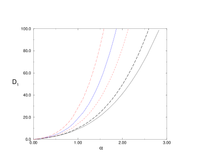
Figure 2: Phase diagram obtained by the decoupling Ansatz for $\tau=0.1,0.5,1.0$ and 2.0. The full black line corresponds to the white noise problem.

Using the expansions (26) obtained for the white noise, we derive the asymptotic behavior of the critical line in the decoupling approximation :

$${\mathcal{D}}_{1}^{c} \simeq 4\alpha\,\,\,\hbox{ for }\alpha\ll 1$$ (46)

$${\mathcal{D}}_{1}^{c} \simeq 3.54\tau\alpha^{4}\,\,\,\hbox{ for }\alpha\gg 1\,.$$ (47)

For small values of the dissipation rate $\alpha$, the critical curve obtained by the decoupling approximation is linear with the same slope as for white noise : comparing equation (46) with the exact expansion (38), we observe that this result is quantitatively correct only if $\tau\ll 1$. For large values of the dissipation rate $\alpha$, equation (47) shows that ${\mathcal{D}}_{1}$ scales as the fourth power of $\alpha$; we recall that for white noise, the asymptotic scaling is ${\mathcal{D}}_{1}^{c}\propto\alpha^{3}$ (see equation (26)). This asymptotic scaling, different from the one obtained in the white noise case, is valid as soon as $\tau\neq 0$, however small $\tau$ may be. This feature will be investigated more specifically in section 6.

Finally, we can study the special case $\alpha=2$. Defining $L=\tau_{1}\Big{(}\Lambda(2,{\mathcal{D}}_{1},\tau_{1})+1\Big{)}$, we find from equations (27) and  (44) that $L$ satisfies

$$L^{3}(1+2L)=\frac{3\,\pi^{3/2}}{4\,\Gamma(\frac{1}{6})^{3}}{\mathcal{D}}_{1}\tau_{1}^{3}\,.$$ (48)

Solving this quartic equation for $L$ leads to the Lyapunov exponent for the critical value $\alpha=2$. In particular, we have

$$\Lambda(2,{\mathcal{D}}_{1},\tau_{1}) \simeq \frac{\sqrt{\pi}}{\Gamma(1/6)}\left(\frac{3{\mathcal{D}}_{1}}{4}\right)^{\frac{1}{3}}-1\simeq 0.289\,\,{\mathcal{D}}_{1}^{\frac{1}{3}}-1\,\,\,\hbox{for }\,\,\,{\mathcal{D}}_{1}\tau_{1}^{3}\ll 1\,,$$ (49)

$$\Lambda(2,{\mathcal{D}}_{1},\tau_{1}) \simeq \left(\frac{\sqrt{\pi}}{\Gamma(1/6)}\right)^{\frac{3}{4}}\left(\frac{3{\mathcal{D}}_{1}}{8\tau_{1}}\right)^{\frac{1}{4}}-1\simeq 0.331\,\left(\frac{{\mathcal{D}}_{1}}{\tau_{1}}\right)^{\frac{1}{4}}-1\,\,\,\hbox{ for }\,\,\,{\mathcal{D}}_{1}\tau_{1}^{3}\gg 1\,.$$ (50)

The polynomial equation (48) interpolates between the white noise solution (equation (49) is identical to equation (27)) and the colored noise scaling with exponent $1/4$ when ${\mathcal{D}}_{1}\tau_{1}^{3}\gg 1$ (equation (50)).

V Effective Fokker-Planck equations for small correlation time

In this section, we study the effective Fokker-Planck equations that are valid when the correlation time $\tau$ of the noise is small. The stationary solutions of these equations allow us to calculate small correlation time approximations of the Lyapunov exponent. In the spirit of hanggirev1 , we derive these approximations from the exact evolution equation (31).

V.1 First order effective Fokker-Planck equation

In the small correlation time approximation, we assume that $\tau\ll 1$ and thus, in equation (31), we have $|t-s|\ll 1$. We then make the following approximation:

$$\exp\left(\int_{s}^{t}f^{\prime}(z(u))\rm{d}u\right)\simeq\exp\big{(}(t-s)f^{\prime}(z(t))\big{)}\,.$$ (51)

Inserting this expression in the functional equation (31) and using equation (28), we obtain an effective Fokker-Planck equation, valid at first order in $\tau$

$$\frac{\partial P_{t}(z)}{\partial t}=-\frac{\partial}{\partial z}\left(f(z)P_{t}(z)\right)+\frac{\Delta}{2}\frac{\partial^{2}}{\partial z^{2}}\Big{(}(1+\tau f^{\prime}(z))P_{t}(z)\Big{)}\,.$$ (52)

We remark that in the limit $\tau\to 0$ this equation reduces to the white noise Fokker-Planck equation. Using the expression (9) for the function $f$, we find that the first order effective Fokker-Planck equation leading to the Lyapunov exponent is given by

$$\frac{\partial P_{t}(z)}{\partial t}=-\frac{\partial}{\partial z}\left((\epsilon-z^{2})P_{t}(z)\right)+\frac{\Delta}{2}\frac{\partial^{2}}{\partial z^{2}}\Big{(}(1-2\tau z)P_{t}(z)\Big{)}\,.$$ (53)

We now solve this effective Fokker-Planck equation in the stationary limit. Introducing the stationary current $J$ we obtain

$$J=(z^{2}-\epsilon)P(z)+\frac{\Delta}{2}\frac{\partial}{\partial z}\Big{(}(1-2\tau z)P(z)\Big{)}\,.$$ (54)

This equation is solved by the variations of constants method. In terms of the parameters

$$z_{0}=\frac{1}{2\tau}\,\,\,\hbox{ and }\,\,\,A=\frac{1-4\tau^{2}\epsilon}{4\tau^{3}\Delta}\,,$$ (55)

the stationary P.D.F. can be written as

$$\hbox{ For }\,z\leq z_{0},\,\,\,P(z) = \frac{2J}{\Delta}|2\tau z-1|^{A-1}\exp\left(\frac{z^{2}}{2\tau\Delta}+\frac{z}{2\tau^{2}\Delta}\right)\,\int_{-\infty}^{z}{\rm d}u\frac{\exp\left(-\frac{u^{2}}{2\tau\Delta}-\frac{u}{2\tau^{2}\Delta}\right)}{|2\tau u-1|^{A}}$$

$$\hbox{ For }\,z\geq z_{0},\,\,\,P(z) = \frac{2J}{\Delta}(2\tau z-1)^{A-1}\exp\left(\frac{z^{2}}{2\tau\Delta}+\frac{z}{2\tau^{2}\Delta}\right)\,\int_{z}^{+\infty}{\rm d}u\frac{\exp\left(-\frac{u^{2}}{2\tau\Delta}-\frac{u}{2\tau^{2}\Delta}\right)}{(2\tau u-1)^{A}}\,.$$ (56)

We remark that when $\tau\to 0$ this P.D.F. becomes identical to the formula (23) derived for white noise. Using equation (56), we can show that $P(z)\simeq\frac{J}{z^{2}}\,\,\,\hbox{ when }\,\,\,z\to\pm\infty\,.$ The behavior of $P(z)$ when $z\to z_{0}$ is as follows:

For $$\,A<1\,,\,\,\,P(z)\sim\frac{1}{|z-z_{0}|^{1-A}}\,,$$ (57)

For $$\,A=1\,,\,\,\,P(z)\sim\ln|z-z_{0}|\,,$$ (58)

For $$\,A>1\,,\,\,\,P(z_{0})=\frac{J}{\tau\Delta(A-1)}\,.$$ (59)

Thus, for $A>0$, the stationary P.D.F. is a positive and normalizable function and the current $J$ is fixed by imposing $\int_{-\infty}^{+\infty}P=1$. The small correlation time approximation breaks down when $A<0$, i.e., when $4\tau^{2}\epsilon>1$; this happens in the case $\epsilon=+1$ and $\tau>1/2.$ In the rest of this section, we consider only the case $\tau<1/2$ : the approximation is then well defined and can be used to study the Lyapunov exponent.

For small noise, $\Delta\ll 1$ and low damping, $\epsilon=1$, we derive a perturbative expansion of the stationary P.D.F. (56) :

$$\Lambda(\epsilon=-1,\Delta,\tau)=\frac{\Delta}{8}+\frac{\Delta^{2}\,\tau\,}{16}+{\mathcal{O}}(\Delta^{3})\,.$$ (60)

We observe that the linear term in $\Delta$ agrees with the exact result (37) if terms of order ${\mathcal{O}}(\tau^{2})$ are neglected. However, the term proportional to $\Delta^{2}$ does not coincide with the exact result even at the first order in $\tau$.

For large noise, $\Delta\gg 1$, and for a given correlation time $\tau$, equation (55) implies that $A\to 0$. From equation (57), we conclude that the stationary P.D.F. becomes more and more localized in the vicinity of $z_{0}$ as $\Delta$ grows : hence $\langle z\rangle\to z_{0}={1}/{2\tau}$ as $\Delta\to\infty.$ Thus, the first order effective Fokker-Planck equation predicts that the Lyapunov exponent saturates to a finite value when the amplitude of the noise grows. This prediction is unphysical and in contradiction with numerical results. The first order effective Fokker-Planck equation is therefore meaningful only for small amplitudes of the noise.

In conclusion, the first order effective Fokker-Planck equation does not provide a good approximation to calculate the Lyapunov exponent. In the next section, we discuss a more sophisticated approach that leads to good results for the small noise regime at least.

V.2 The ‘Best Fokker-Planck Equation’

This approximation has been first proposed in lindcol1 . Starting from an approximate integro-differential equation for the P.D.F. valid at first order in the noise amplitude, the evolution kernel is calculated by a resummation to all orders in the noise correlation time. This procedure results in an effective Fokker-Planck equation, called the Best Fokker-Planck Equation (B.F.P.E.). Although this equation is not free from inconsistencies marchesoni , it provides in some cases useful insights that agree qualitatively with numerical simulations. (Another approach, that we shall not follow here, is to reject the assumption of stationarity and to study non-conventional diffusion regimes of a Fokker-Planck equation with a time-dependent diffusion constant tsironis .)

Following hanggirev1 , we derive the B.F.P.E. approximation from the exact functional evolution equation (31). In the B.F.P.E. approach the amplitude $\Delta$ of the noise is supposed to be small and contributions of order $\Delta^{n}$ with $n\geq 2$ are neglected. In order words, the exact evolution equation (31) is replaced by

$$\frac{\partial P_{t}(z)}{\partial t}=-\frac{\partial}{\partial z}\left(f(z)P_{t}(z)\right)+\frac{{\Delta}}{2\tau}\frac{\partial^{2}}{\partial z^{2}}\int_{0}^{t}\rm{d}s\,\,\exp\left(-|t-s|/\tau\right)\exp\left(\int_{s}^{t}f^{\prime}({\bf\bar{z}}(u))\rm{d}u\right)\,\left\langle\delta(z(t)-z)\right\rangle\,,$$ (61)

where ${\bf\bar{z}}(u)$ is the solution of the deterministic ( i.e., noiseless) equation

$$\frac{{\rm d}{\bf\bar{z}}}{{\rm d}u}=f\left({\bf\bar{z}}(u)\right)\,\,\,\hbox{ with }\,\,\,{\bf\bar{z}}(t)=z\,.$$ (62)

Substituting this equation for ${\bf\bar{z}}$ in equation (61), we derive the B.F.P.E.

$$\frac{\partial P_{t}(z)}{\partial t}=-\frac{\partial}{\partial z}\left(f(z)P_{t}(z)\right)+\frac{{\Delta}}{2}\frac{\partial^{2}}{\partial z^{2}}\Big{(}D_{t}(z)\,P_{t}(z)\Big{)}\,\,\,\,\hbox{ with }\,\,\,D_{t}(z)=f(z)\int_{0}^{t}\rm{d}s\,\,\frac{\exp\left(-|t-s|/\tau\right)}{\tau f\left({\bf\bar{z}}(s)\right)}\,.$$ (63)

The space and time dependent diffusion factor $D_{t}(z)$ can be explicitly evaluated for $f(z)=\epsilon-z^{2}$. In the long time limit $t\to\infty$, we obtain endnote

$$\frac{\partial P_{t}(z)}{\partial t}=-\frac{\partial}{\partial z}\left(f(z)P_{t}(z)\right)+\frac{{\Delta}}{2}\frac{\partial^{2}}{\partial z^{2}}\Big{(}D(z)P_{t}(z)\Big{)}\,\,\,\,\hbox{ with }\,\,\,D(z)=\frac{2\tau^{2}z^{2}-2\tau z+1-2\tau^{2}\epsilon}{1-4\tau^{2}\epsilon}\,.$$ (64)

The effective diffusion coefficient $D(z)$ is everywhere positive when $\epsilon=-1$ or 0 for all values of $\tau$. When $\epsilon=1$, $D(z)$ is everywhere positive only if $\tau<1/2$. In all these cases, we obtain

$$P(z)=\frac{2J}{\Delta}\exp\left(-4\tau Az\right)\,D(z)^{-2A-1}\int_{-\infty}^{z}{\rm d}u\exp\left(4\tau Au\right)D(u)^{2A}\,,$$ (65)

where $A$ was defined in equation (55). The value of $J$ is again fixed by normalizing $P$. Again, when $\tau\to 0$, this expression becomes identical to the formula (23) for the P.D.F. obtained in the white noise case. From this expression of the stationary P.D.F. we derive the expression of the Lyapunov exponent:

$$\Lambda(\epsilon,\Delta,\tau)=\frac{\int_{-\infty}^{\infty}{\rm d}z\,z\,\exp\left(-4\tau Az\right)\,D(z)^{-2A-1}\int_{-\infty}^{z}{\rm d}u\,\exp\left(4\tau Au\right)D(u)^{2A}}{\int_{-\infty}^{\infty}{\rm d}z\exp\left(-4\tau Az\right)\,D(z)^{-2A-1}\int_{-\infty}^{z}{\rm d}u\exp\left(4\tau Au\right)D(u)^{2A}}\,,$$ (66)

where the integral in the numerator is defined in the sense of principal parts. This closed formula can be used for a numerical evaluation of the Lyapunov exponent in the B.F.P.E. approximation (see figure 3).

The perturbative expansion of the Lyapunov exponent (66) when $\Delta\ll 1$ and $\epsilon=1$ is given by

$$\Lambda(\epsilon=-1,\Delta,\tau)=\frac{\Delta}{8(1+4\tau^{2})}+\frac{\Delta^{2}\,\tau\,(1+3\tau^{2})}{16(1+4\tau^{2})^{2}}+{\mathcal{O}}(\Delta^{3})\,.$$ (67)

Comparing this expression with the exact result (37), we observe that the first term of this expansion with respect to $\Delta$ is correct. The B.F.P.E. yields the exact result to all orders in $\tau$ and performs indeed a complete resummation with respect to the correlation time. However, the term in $\Delta^{2}$ does not agree with the exact result, even in the $\tau\to 0$ limit. We recall that the BFPE approximation is intrinsically a small noise expansion and we see clearly, in this specific example, that this approximation is not valid at second order in the noise amplitude. This agrees with the general analysis of marchesoni that the BFPE can not be used for moderate values of the noise because the neglected non-Fokker Planck terms have a contribution of the same order as the terms obtained after resummation with respect to the correlation time.

VI Adiabatic limit for large correlation time

In the previous section, we studied small correlation time effective equations which yield fairly good approximations for the critical line for small-to-moderate values of the noise amplitude. But these approximations always break down when $\alpha\sim 1/\tau$: a specific approximation scheme is therefore needed for this range and will become more and more relevant as $\tau$ grows.

In this last section, we thus study the large $\tau$ case. When the correlation time is large, the Ornstein-Uhlenbeck noise becomes a slow variable and the dynamics of the random variable $z$ can be simplified. We shall first perform an elementary adiabatic elimination that yields an expression of the Lyapunov exponent in the $\tau\to\infty$ limit. Then, we show that these results can be obtained in a more systematic manner thanks to the Unified Colored Noise Approximation (UCNA).

When $\tau$ is large, the noise $\xi(t)$ is slowly varying and we make the approximation that $z$ keeps adjusting itself to the stationary solution of equation (8). We consider here only the domain $\alpha>2$ (i.e., $\epsilon=1$) for which the small correlation time expansions do not provide reliable results. Thus, we study the limiting case where the noise $\xi$ is quenched; the equation (8) then reduces to

$$\dot{z}=1-z^{2}+\xi\,,$$ (68)

where $\xi$ is a time-independent Gaussian random variable of variance $\Delta/(2\tau)$. The value of $z$ is then given by the stable fixed point of equation (68) if such a solution exists. We must distinguish two cases:

• if $\xi>-1$, then $z=+\sqrt{\xi+1}$ (the solution $z=-\sqrt{\xi+1}$ is unstable);

• if $\xi<-1$, then equation (68) has no fixed point. The random variable $z$ is given by $z(t)=A\,\mathrm{cotan}(At)$ with $A^{2}=-(\xi+1)$. This running solution implies that $z$ is distributed over the whole real axis.

From this discussion, we conclude that the distribution of $z$ is given by

$$\mathrm{For}\,\,z>0, P(z)=2\sqrt{\frac{\tau}{\pi\Delta}}z\exp\left(-\tau(z^{2}-1)^{2}/\Delta\right)+\sqrt{\frac{\tau}{\pi\Delta}}\int_{-\infty}^{-1}\frac{\sqrt{-\xi-1)}}{\pi(z^{2}-\xi-1)}\exp\left(-\tau\xi^{2}/\Delta\right)\mathrm{d}\xi\,,$$ (69)

$$\mathrm{for}\,\,z<0, P(z)=\sqrt{\frac{\tau}{\pi\Delta}}\int_{-\infty}^{-1}\frac{\sqrt{-\xi-1)}}{\pi(z^{2}-\xi-1)}\exp\left(-\tau\xi^{2}/\Delta\right)\mathrm{d}\xi\,.$$

This P.D.F. consists of two parts: one term is of Lorentzian type and is an even function of z; the other term exists only for $z>0$ and is a rapidly decaying function. This contribution provides a strictly positive value for the mean value of $z$. Using equation (69), we calculate the Lyapunov exponent

$$\Lambda(\epsilon=1,\Delta,\tau)=\langle z\rangle=2\sqrt{\frac{\tau}{\pi\Delta}}\int_{0}^{\infty}z^{2}\exp\left(-\tau(z^{2}-1)^{2}/\Delta\right)\mathrm{d}z\simeq\frac{\Gamma(3/4)}{2\sqrt{\pi}}\Big{(}\frac{\Delta}{\tau}\Big{)}^{1/4}\,\,\,\,\,\,\,\,\mathrm{when}\,\,\frac{\Delta}{\tau}\gg 1\,.$$ (70)

This simple adiabatic approximation provides the behavior of the Lyapunov exponent for large amplitude of the noise and it predicts a scaling in agreement with the decoupling Ansatz (see equation (47)). Moreover, it explains the existence of long tails for the P.D.F. of $z$ near infinity ($P(z)\sim 1/z^{2}$ when $|z|\to\infty)$ and the asymmetry in $P(z)$ for $z\to-z$. Because of this asymmetry that favors positive values of $z$, the Lyapunov exponent, $\langle z\rangle$, is always strictly positive. Using equation (70), we obtain the asymptotic behavior of the critical curve for large values of the noise amplitude,

$${\mathcal{D}}_{1}^{c}\simeq\left(\frac{\alpha\sqrt{\pi}}{\Gamma(3/4)}\right)^{4}\tau_{1}\simeq 4.37\,\alpha^{4}\tau_{1}\,.$$ (71)

This approximation is fairly accurate even from quantitative point of view and provides a good approximation of the critical noise amplitude even at moderate values: this can be seen in figure 3, where the expression (71) is compared with the critical curve, computed numerically. Moreover, the asymptotic behavior in equation (71) agrees well with the prediction of the decoupling Ansatz, equation (47).

For the special case $\alpha=2$, we can repeat the above calculations and find that

$$\Lambda(2,{\mathcal{D}}_{1},\tau_{1})=\frac{\Gamma(3/4)}{2\sqrt{\pi}}\Big{(}\frac{{\mathcal{D}}_{1}}{\tau_{1}}\Big{)}^{1/4}-1\simeq 0.345\Big{(}\frac{{\mathcal{D}}_{1}}{\tau_{1}}\Big{)}^{1/4}-1\,.$$ (72)

This expression is very similar to equation (50) obtained by decoupling Ansatz. However the limit $\tau\to 0$ is ill-defined here; this is not a surprise because the adiabatic elimination makes sense only if $\tau$ is large.

Figure 3: Various approximations for the phase digram at $\tau=1$. The critical curve, computed numerically, is plotted in full line with black circles ($\bullet$). The small and large $\tau$ expansions, equations (37) and (71) respectively, are drawn with dashed lines. The decoupling approximation, equation (45), is plotted with a dot-dashed line. The BFPE approximation is represented with $\triangle$.

Finally, we show that the adiabatic elimination can be performed in a systematic manner by using the simplest version of the unified colored noise approximation hanggirev1 ; JungHanggi ; schimansky2 (for more sophisticated UCNA schemes, see e.g., madureira ; wio ). Taking the time derivative of equation (8) and using equation (11), we obtain

$$\ddot{z}=f^{\prime}(z)\dot{z}+\dot{\xi}=f^{\prime}(z)\dot{z}-\frac{1}{\tau}\xi+\frac{1}{\tau}\eta\,.$$ (73)

Using again equation (8) to express the Ornstein-Uhlenbeck noise in terms of $z$ and the white noise $\eta$, we derive the following second-order nonlinear Langevin equation driven by white noise:

$$\frac{d^{2}z}{dT^{2}}+\gamma_{\tau}(z)\frac{dz}{dT}-f(z)=\frac{1}{\tau^{1/4}}\eta(T)\,\,\,\,\hbox{ where }\,\,\,\gamma_{\tau}(z)=\frac{1}{\sqrt{\tau}}-\sqrt{\tau}f^{\prime}(z)\,,$$ (74)

where the new scale of time is $T=t/\sqrt{\tau}$. The effective damping coefficient $\gamma_{\tau}(z)$ diverges when $\tau\to 0$ and $\tau\to\infty$. After an adiabatic elimination of the inertial term (valid for $2\tau z+1\gg\sqrt{\tau}$) the following effective stochastic equation is obtained:

$$\frac{dz}{dT}=\frac{\epsilon-z^{2}}{\gamma_{\tau}(z)}+\frac{1}{\tau^{1/4}\gamma_{\tau}(z)}\eta(T)\,,\,\,\,\,\hbox{ with }\,\,\,\,\gamma_{\tau}(z)=\frac{1}{\sqrt{\tau}}+2\sqrt{\tau}z\,.$$ (75)

The solution of the associated Fokker-Planck equation leads to the stationary P.D.F., which in the domain of validity of the UCNA is given by

$$P(z)={\mathcal{N}}|2\tau z+1|\exp-\frac{2}{\Delta}\left(\frac{\tau z^{4}}{2}+\frac{z^{3}}{3}-\epsilon\tau z^{2}-\epsilon z\right)\,\,\hbox{ for }\,z\geq-\frac{1}{2\tau}\,.$$ (76)

The constant ${\mathcal{N}}$ is fixed by the normalization condition on $P(z)$. From this expression we deduce that the Lyapunov exponent is given by

$$\Lambda(\epsilon=1,\Delta,\tau)=\frac{\int_{0}^{\infty}z|2\tau z+1|\exp-\frac{2}{\Delta}\left(\frac{\tau z^{4}}{2}+\frac{z^{3}}{3}-\epsilon\tau z^{2}-\epsilon z\right)\mathrm{d}z}{\int_{0}^{\infty}|2\tau z+1|\exp-\frac{2}{\Delta}\left(\frac{\tau z^{4}}{2}+\frac{z^{3}}{3}-\epsilon\tau z^{2}-\epsilon z\right)\mathrm{d}z}\,.$$ (77)

Here, the range of the variable $z$ is taken from 0 to $\infty$ instead of $z\geq-\frac{1}{2\tau}$ (this is a good approximation when $\tau$ is large). For $\epsilon=1$ and $\Delta\gg 1$, this expression scales as $({\Delta}/{\tau})^{1/4}$, in agreement with the behavior predicted by the decoupling Ansatz and the adiabatic elimination. For the special case $\alpha=2$, equations (20 and 77) lead to

$$\Lambda(2,{\mathcal{D}}_{1},\tau_{1})=\frac{1}{\tau_{1}}\frac{\int_{0}^{\infty}z|2z+1|\exp-\frac{2}{{\mathcal{D}}_{1}\tau_{1}^{3}}\left(\frac{z^{4}}{2}+\frac{z^{3}}{3}\right)\mathrm{d}z}{\int_{0}^{\infty}|2z+1|\exp-\frac{2}{{\mathcal{D}}_{1}\tau_{1}^{3}}\left(\frac{z^{4}}{2}+\frac{z^{3}}{3}\right)\mathrm{d}z}-1 \simeq \frac{1}{\Gamma(2/3)}\left(\frac{3{\mathcal{D}}_{1}}{2}\right)^{\frac{1}{3}}-1\hbox{ for }\,\,\,{\mathcal{D}}_{1}\tau_{1}^{3}\ll 1\,,$$ (78)

$$\simeq \frac{\Gamma(3/4)}{\sqrt{\pi}}\Big{(}\frac{{\mathcal{D}}_{1}}{\tau_{1}}\Big{)}^{1/4}-1\hbox{ for }\,\,\,{\mathcal{D}}_{1}\tau_{1}^{3}\gg 1$$ (79)

Thus, the UCNA approximation permits an interpolation between small and large values of the correlation time. The predicted behavior matches the white noise scaling for small $\tau$, and the colored noise scaling at large $\tau$. We remark that prefactors in equations (78 and 79) are different from those obtained in equations (27) and (70), respectively; this is due to the fact that in the UCNA the stationary current vanishes : the running solution of $z$ are overlooked and therefore this approximation does not describe satisfactorily the tails of the P.D.F. of $z$.

This study of the $\tau\to\infty$ limit shows that the absorbing phase becomes more and more stable as the correlation time increases. Besides, it confirms that the existence of a time correlation of the noise renders the critical curve steeper and modifies its scaling behavior for large values of the noise amplitude.

VII Conclusion

The long time behavior of the stochastic oscillator with random frequency is controlled by the sign of the Lyapunov exponent. In the case of a white noise perturbation, this exponent can be calculated exactly and the phase diagram of the stochastic oscillator can then be rigorously determined. The aim of this work is to study the effects of time correlations on the noise-induced bifurcation of the stochastic oscillator. In the case of an Ornstein-Uhlenbeck noise, an exact calculation seems to be out of reach and therefore we use various approximation schemes in order to derive analytical expressions for the Lyapunov exponent and to draw the phase diagram. Since the different approximations have distinct regions of validity, their study has allowed us to derive a global picture of the behavior of the system in the parameter space. In particular, we have derived the scaling behavior of the phase boundary in regions where the amplitude of the noise is small or large. Our results agree fairly well with numerical simulations and with exact perturbative expansions. These comparisons allow us to test the validity of the different approximation schemes.

We remark that the effective first order equation (8), that we have used to calculate the Lyapunov exponent, can be interpreted as describing an overdamped Brownian particle driven by colored noise in a metastable potential. For such a system, a fundamental and extensively studied quantity is the mean escape-time of the particle vankampen from the well. The relation between the Lyapunov exponent and this mean escape-time deserves to be clarified. In particular, one could then use path-integral techniques bray ; dykman to study the phase diagram of the random frequency oscillator. The variation of the Lyapunov exponent with the correlation time of the noise could then be related to the phenomenon of noise enhanced stability in metastable states dubkov .

The study carried out here for the oscillator with multiplicative noise can be adapted to other stochastic systems. For example, Schimansky-Geier et al. schimansky have shown that the random Duffing oscillator with additive noise undergoes a subtle phase transition that does not manifest itself in the stationary P.D.F. (which is simply given by the Gibbs-Boltzmann formula) but affects the properties of the random attractor in phase space. This problem is mathematically equivalent to the noise-induced bifurcation of a linear oscillator subject to a multiplicative colored noise. This noise has a finite correlation time and if we approximate it by an Ornstein-Uhlenbeck process, the system becomes identical to the one studied here.

It has been suggested recently vandenbroeck that the Poisson process may be suitable as a paradigm study of time correlation effects in random dynamical systems. In fact, in many cases, a complete analytical study can be carried out for a random variable driven by Poisson noise, but not when the stochastic force is an Ornstein-Uhlenbeck process. We have indeed carried out the exact calculation of the Lyapunov exponent of a random frequency oscillator subject to a Poisson noise and obtained the exact phase diagram of the system orantin . The results are in qualitative agreement with those found here with an Ornstein-Uhlenbeck noise.

Appendix A Derivation of the effective Langevin equation

In this appendix, we show that the calculation of the Lyapunov exponent can be reduced to solving a nonlinear first order Langevin equation. We introduce the function $y(t)=\frac{\dot{x}}{x}$, that satisfies

$$\frac{\mathrm{d}y}{\mathrm{d}t}=-(1+\alpha y+y^{2})+\xi(t)\,.$$ (80)

Using the fact that

$$\frac{1}{2}\log(2E)=\log x+\frac{1}{2}\log\left(y^{2}+1\right)\,,$$ (81)

where $E=\frac{\dot{x}^{2}}{2}+\frac{x^{2}}{2}$ is the total energy of the system, we derive the following identity:

$$\frac{1}{2}\frac{d}{dt}\langle\log E\rangle=\langle y\rangle_{t}+\frac{1}{2}\frac{d}{dt}\left\langle\log\left(y^{2}+1\right)\right\rangle_{t}\,.$$ (82)

This identity implies that the Lyapunov exponent is given by

$$\Lambda(\alpha,{\mathcal{D}}_{1},\tau_{1})=\frac{1}{2}\lim_{t\to\infty}\frac{d}{dt}\langle\log E\rangle=\lim_{t\to\infty}\left(\langle y\rangle_{t}+\frac{1}{2}\frac{d}{dt}\left\langle\log(y^{2}+1)\right\rangle_{t}\right)\,.$$ (83)

We introduce an auxiliary variable $z$ defined as

$$z=\frac{\dot{x}}{x}+\frac{\alpha}{2}=y+\frac{\alpha}{2}\,.$$ (84)

Eliminating $y$ from equation (80), we obtain

$$\dot{z}=\frac{\alpha^{2}}{4}-1-z^{2}+\xi(t)\,.$$ (85)

We now show that the dissipation parameter can be eliminated from this equation by a suitable redefinition of the parameters involved in the problem. We have to distinguish three cases:

• Underdamped case ($\alpha<2$): in terms of $t:=\sqrt{1-\frac{\alpha^{2}}{4}}\,\,t$, the evolution equation of $z$ becomes

  $$\dot{z}=-1-z^{2}+\xi(t)\,,$$ (86)

  where $\xi$ is an Ornstein-Uhlenbeck noise of amplitude and correlation time given by

  $$\Delta=\frac{{\mathcal{D}}_{1}}{\left(1-\frac{\alpha^{2}}{4}\right)^{3/2}}\,,\,\,\,\,\,\,{\hskip 28.45274pt}\tau=\tau_{1}\,\sqrt{1-\frac{\alpha^{2}}{4}}\,.$$ (87)

• Critical damping ($\alpha=2$): the evolution of $z$ is given by

  $$\dot{z}=-z^{2}+\xi(t)\,.$$ (88)

  We can rescale the time variable either as $t:={\mathcal{D}}_{1}^{1/3}t$, or as $t:=t/\tau_{1}$. The amplitude and correlation time of $\xi$ are then given, respectively, by

  $$\Delta =1\,,\,\,\,\,\,\,{\hskip 28.45274pt}\tau={\mathcal{D}}_{1}^{1/3}\tau_{1}\,.$$ (89)

  or $$\Delta ={\mathcal{D}}_{1}\tau_{1}^{3}\,,\,\,\,\,\,\,{\hskip 28.45274pt}\tau=1\,.$$ (90)

  We notice that in the critical damping case there is only one free parameter in the problem (in the white noise limit $\tau_{1}=0$, no free parameter is left).

• Overdamped case ($\alpha>2$): in terms of $t:=\sqrt{\frac{\alpha^{2}}{4}-1}\,\,t$, the evolution equation of $z$ becomes

  $$\dot{z}=1-z^{2}+\xi(t)\,,$$ (91)

  where the amplitude and correlation time of $\xi$ are given by

  $$\Delta=\frac{{\mathcal{D}}_{1}}{\left(\frac{\alpha^{2}}{4}-1\right)^{3/2}}\,,\,\,\,\,\,\,{\hskip 28.45274pt}\tau=\tau_{1}\,\sqrt{\frac{\alpha^{2}}{4}-1}\,.$$ (92)

We have thus shown that the calculation of the Lyapunov exponent of the linear oscillator with random frequency can be reduced to the study of the following equation

$$\dot{z}=\epsilon-z^{2}+\xi(t)\,,$$ (93)

with

$$\epsilon=\rm{sign}(\alpha-2)\,,$$ (94)

i.e., $\epsilon=-1,0$ or 1 when $\alpha<2$, $\alpha=2$ and $\alpha>2$ respectively. Using equation (83) and taking into account the rescaling of time, we conclude that

$$\Lambda(\alpha,{\mathcal{D}}_{1},\tau_{1})=\kappa\Lambda(\epsilon,\Delta,\tau)-\frac{\alpha}{2}\,,$$ (95)

where we have defined

$$\Lambda(\epsilon,\Delta,\tau)=\lim_{t\to\infty}\left(\langle z\rangle_{t}+\frac{1}{2}\frac{d}{dt}\left\langle\log\left((z-\frac{\alpha}{2})^{2}+1\right)\right\rangle_{t}\right)\,,$$ (96)

and the coefficient $\kappa$ is equal to $\sqrt{1-\frac{\alpha^{2}}{4}}\,$, ${\mathcal{D}}_{1}^{1/3}$ or $\sqrt{\frac{\alpha^{2}}{4}-1}\,$ when $\alpha<2$, $\alpha=2$ or $\alpha>2$, respectively. We remark that when $t\to\infty$,

$$\left\langle\log\left((z-\frac{\alpha}{2})^{2}+1\right)\right\rangle_{t}-\left\langle\log\left(z^{2}+1\right)\right\rangle_{t}\to\left\langle\log\frac{(z-\frac{\alpha}{2})^{2}+1}{z^{2}+1}\right\rangle\,,$$ (97)

where the average on the right hand side is taken with respect to the stationary P.D.F. of $z$ and does not depend on time. Therefore, equation (96) is equivalent to

$$\Lambda(\epsilon,\Delta,\tau)=\lim_{t\to\infty}\left(\langle z\rangle_{t}+\frac{1}{2}\frac{d}{dt}\left\langle\log\left(z^{2}+1\right)\right\rangle_{t}\right)\,,$$ (98)

which is identical to equation (16).

Appendix B Proof of equation (17)

We now derive the identity (17) for the Lyapunov exponent that involves only the stationary P.D.F. of $z$. In all the cases considered in this work, we obtain an effective Fokker-Planck equation of the type :

$$\frac{\partial P_{t}(z)}{\partial t}=-\frac{\partial}{\partial z}\left(f(z)P_{t}(z)\right)+\frac{\Delta}{2}\frac{\partial^{2}}{\partial z^{2}}\Big{(}D(z)P_{t}(z)\Big{)}\,.$$ (99)

In the stationary limit, we have

$$J=-f(z)P(z)+\frac{\Delta}{2}\frac{d}{dz}\Big{(}D(z)P(z)\Big{)}\,,$$ (100)

where $J$ represents the stationary current. After an integration by parts, we deduce from equation (99) that

$$\frac{d}{dt}\left\langle\log(z^{2}+1)\right\rangle_{t}=\int_{-\infty}^{+\infty}{\rm d}z\frac{2z}{z^{2}+1}\left(-f(z)P_{t}(z)+\frac{\Delta}{2}\frac{d(D(z)P_{t}(z))}{dz}\right)\,.$$ (101)

Thus, we have

$$\langle z\rangle_{t}+\frac{1}{2}\frac{d}{dt}\left\langle\log(z^{2}+1)\right\rangle_{t}=\int_{-\infty}^{+\infty}\,z\Big{(}P_{t}(z)-\frac{-f(z)P_{t}(z)+\frac{\Delta}{2}\frac{d}{dz}(D(z)P_{t}(z))}{z^{2}+1}\Big{)}{\rm d}z\,.$$ (102)

Taking the stationary limit and using equation (100), we find

$$\lim_{t\to\infty}\left(\langle z\rangle_{t}+\frac{1}{2}\frac{d}{dt}\left\langle\log(z^{2}+1)\right\rangle_{t}\right)=\int_{-\infty}^{+\infty}\,z\left(P(z)-\frac{J}{z^{2}+1}\right){\rm d}z\,.$$ (103)

Combining equations (98) and (103), we obtain the following identity for the Lyapunov exponent

$$\Lambda(\epsilon,\Delta,\tau)=\int_{-\infty}^{+\infty}\,z\left(P(z)-\frac{J}{z^{2}+1}\right){\rm d}z=\int_{-\infty}^{+\infty}\,zP(z){\rm d}z\,,$$ (104)

where the last equality has to be understood in the sense of calculating the ’principal part’ of the integral, i.e.,

$$\int_{-\infty}^{+\infty}\,z\,P(z){\rm d}z=\lim_{M\to+\infty}\int_{-M}^{+M}\,z\,P(z){\rm d}z\,.$$ (105)

Thanks to the formula (104), the Lyapunov exponent is expressed in terms of the stationary P.D.F. of $z$ and equation (104) can be rewritten as

$$\Lambda=\langle\,z\,\rangle\,,$$ (106)

which is identical to equation (17). We emphasize that the first moment of the stationary P.D.F. needs to be defined only in the sense of the principal values.

References

- (1) N.G. van Kampen, Stochastic Processes in Physics and Chemistry (North-Holland, Amsterdam, 1992).
- (2) C. W. Gardiner, Handbook of stochastic methods (Springer-Verlag, Berlin, 1994).
- (3) V.S. Anishchenko, V.V. Astakhov, A.B. Neiman, T.E. Vadivasova and L. Schimansky-Geier, Nonlinear Dynamics of Chaotic and Stochastic Systems (Springer-Verlag, Berlin, 2002).
- (4) H. Horsthemke and R. Lefever, Noise Induced Transitions (Springer-Verlag, Berlin, 1984).
- (5) R. Berthet, S. Residori, B. Roman and S. Fauve, Phys. Rev. Lett. 33, 557 (2002); F. Pétrélis, S. Aumaître, Eur. Phys. J. B 34 281 (2003)
- (6) M. a. Muñoz, Nonequilibrium Phase transitions and Multiplicative Noise in Advances in Condensed Matter and Statistical Mechanics, edited by E. Korutcheva and R. Cuerno (Nova Science Publishers, 2004) cond-mat/0303650.
- (7) A. Pikovsky, M. Rosenblum, and J. Kurths, Synchronization, A Universal Concept in Nonlinear Sciences (Cambridge University Press, 2001).
- (8) M. Lücke and F. Schank, Phys. Rev. Lett. 54, 1465 (1985); M. Lücke, in Noise in Dynamical Systems, Vol. 2: Theory of Noise-induced Processes in Special Applications, edited by F. Moss and P.V.E. Mc Clintock (Cambridge University Press, Cambridge, 1989).
- (9) W. Ebeling, H. Herzel, R. Richert, L. Schimansky-Geier, Z. angew. Math. Mech. 66 141 (1986).
- (10) H.W. Rong, G. Meng, X.D. Wang, W. Xu and T. Fang, Journal of Sound and Vibration 210, 483 (1998).
- (11) H. Rong, W. Xu and T. Fang, Journal of Sound and Vibration 283, 1250 (2005).
- (12) Z. L. Huang, W. Q. Zhu, Y. Q. Ni and J. M. Ko, Journal of Sound and Vibration 254, 245 (2002).
- (13) W. C. Xie, Journal of Sound and Vibration 289, 171 (2006).
- (14) A. H. Nayfeh, Perturbation Methods (John Wiley, 1973); A. H. Nayfeh, D. T. Mook, Nonlinear Oscillations (John Wiley, 1979).
- (15) L. Arnold, Random Dynamical Systems (Springer-Verlag, Berlin, 1998).
- (16) R. Zillmer and A. Pikovsky, Phys. Rev. E 67 061117 (2003).
- (17) R.C. Bourret, Physica 54, 623 (1971); R.C. Bourret, U. Frisch and A. Pouquet, Physica 65, 303 (1973).
- (18) K. Mallick and P. Marcq, Eur. Phys. J. B 36, 119 (2003).
- (19) K. Mallick and P. Marcq, Eur. Phys. J. B 38, 99 (2004).
- (20) D. Hansel and J.F. Luciani, J. Stat. Phys. 54, 971 (1989).
- (21) L. Tessieri and F.M. Izrailev, Phys. Rev. E 62, 3090 (2000).
- (22) P. Imkeller and C. Lederer, Dyn. and Stab. Syst. 14, 385 (1999).
- (23) K. Mallick and P. Marcq, Phys. Rev. E 66 041113 (2002).
- (24) K. Mallick and P. Marcq, J. Stat. Phys 119, 1-33 (2005).
- (25) S. Aumaître, F. Pétrélis and K. Mallick, Phys. Rev. Lett. 95 064101 (2005).
- (26) P. Hänggi, in Noise in Dynamical Systems, Vol. 1, edited by F. Moss and P.V.E. Mc Clintock (Cambridge University Press, Cambridge, 1989).
- (27) M. San Miguel and J. M. Sancho, in Noise in Dynamical Systems, Vol. 1, edited by F. Moss and P.V.E. Mc Clintock (Cambridge University Press, Cambridge, 1989).
- (28) P. Jung and P. Hänggi, Phys. Rev. A 35, 4464 (1987).
- (29) P. Hänggi and P. Jung, Adv. Chem. Phys. 89, 239 (1995).
- (30) V. Wihstutz, in Stochastic dynamics, edited by H. Crauel and M. Gundlach (Springer Verlag, New-York, 1999).
- (31) K. Lindenberg and B.J. West, Physica A 119, 485 (1983); K. Lindenberg and B.J. West, Physica A 128, 25 (1984).
- (32) P. Hänggi, F. Marchesoni and P. Grigolini, Z. Phys. B 56, 333 (1984); F. Marchesoni, Phys. Rev. A 36, 4050 (1987).
- (33) G.P. Tsironis and P. Grigolini, Phys. Rev. Lett. 61, 7 (1988).
- (34) We remark that the B.F.P.E. can also be derived using the original operator formalism used in lindcol1 but we preferred here to use a systematic approach in which the approximations are derived from the exact functional equation (31).
- (35) L. H’walisz, P. Jung, P. Hänggi, P. Talkner and L. Schimansky-Geier, Z. Phys. B 77, 471 (1989).
- (36) A. J. R. Madureira, P. Hänggi, V. Buonomano and W. A. Rodrigues, Jr. Phys. Rev. E 51, 3849 (1995)
- (37) F. Castro, A. D. S nchez and H. S. Wio Phys. Rev. Lett. 75, 1691 (1995); F. Castro, H. S. Wio and G. Abramson, Phys. Rev. E 52, 159 (1995).
- (38) A. J. Bray and A. J. Mckane, Phys. Rev. Lett. 62, 493 (1989).
- (39) M. I. Dykman, Phys. Rev. A 42, 2020 (1990).
- (40) A. A. Dubkov, N. V. Agudov and B. Spagnolo, Phys. Rev. E 69, 061103 (2004).
- (41) L. Schimansky-Geier and H. Herzel, J. Stat. Phys. 70, 141 (1993).
- (42) I. Bena, C. Van den Broeck, R. Kawai and K. Lindenberg, Phys. Rev. E 66 045603(R) (2002); Phys. Rev. E 68, 041111 (2003); cond-mat/0501499.
- (43) K. Mallick and N. Orantin, in preparation.