Quasiparticle spectral weights of Gutzwiller-projected high $T_{c}$ superconductors

Abstract

We analyze the electronic Green’s functions in the superconducting ground state of the $t$–$J$ model using Gutzwiller-projected wave functions, and compare them to the conventional BCS form. Some of the properties of the BCS state are preserved by the projection: the total spectral weight is continuous around the quasiparticle node and approximately constant along the Fermi surface. On the other hand, the overall spectral weight is reduced by the projection with a momentum-dependent renormalization, and the projection produces electron-hole asymmetry in renormalization of the electron and hole spectral weights. The latter asymmetry leads to the bending of the effective Fermi surface which we define as the locus of equal electron and hole spectral weight.

I Introduction

Shortly after the discovery of superconductivity in copper-oxyde compounds,bednorz86 Anderson proposed a Gutzwiller-projected BCS wave function which would describe the superconducting ground state of high-temperature superconductors.anderson87 The variational approach to superconducting cuprates based on Anderson’s original proposal has since had a lot of success, while the strong Coulomb repulsion and the non-perturbative nature of the problem make other approaches extremely difficult. Interest in projected wave functions as variational ground states for cuprate superconductors was initiated by several research groups in late 80’s gros88 ; yokoyama88 and lead to a considerable activity in the field. The projected wave functions show large overlap with exact ground states on small clusters and have low variational energies for the $t\text{--}J$ model.hasegawa89 ; becca00 Furthermore, several experimental properties of cuprates like the zero-temperature phase diagram and d-wave pairing symmetry are extremely well predicted within this approach.paramekanti0103 ; rmft

Due to considerable progress of the experimental technique of Angle Resolved Photoemission Spectroscopy (ARPES) on cuprates, more and more high-quality data on the low-lying spectral properties of these compounds have been made available in recent years.ARPES Experimentally, the low-energy excitations of superconducting cuprates are known to resemble BCS quasiparticles (QPs).matsui03 It is therefore interesting to theoretically explore the wave function of projected QP excitations and compare them to unprojected BCS QPs. The most apparent differences are the the doping dependency of the nodal Fermi velocity and the renormalizations of the nodal QP spectral weight and of the current carried by QPs.paramekanti0103 ; yunoki05 ; yunoki05prl ; edegger06 ; nave06 In the present paper we further analyze the properties of the superconducting ground state and the QP excitations with the Variational Monte Carlo technique (VMC).gros78 We calculate the equal-time Green’s functions, both normal and anomalous, in the Gutzwiller-projected state and derive from them the QP spectral weights for addition and removal of an electron at zero temperature. The main conclusion of our study is that, due to a non-trivial interplay of superconductivity and strong Coulomb repulsion (projection), the electron and hole spectral weights are renormalized differently. A natural way to describe this asymmetry is to define the “effective Fermi surface” as the locus of points where the electron and the hole spectral weights are equal. Thus defined Fermi surface acquires an additional outward bending in the anti-nodal region as compared to the original unprojected Fermi surface. This bending is a signature of a deviation from the BCS theory and may be responsible for the shape of the Fermi surface observed in ARPES experiments. The validity of Luttinger’s ruleluttinger61 in strongly interacting and superconducting materials has been questioned experimentally and theoretically recently.ARPES ; sensarma06 ; gros06 Our findings provide further indication of its inapplicability in strongly correlated superconductors.

The paper is organized as follows. Section II contains the definition of the model and wave functions used in our calculations. In Section III we first present some exact relations for projected wave functions, we then describe our results on the QP spectral weights. Section IV is devoted to the calculation of the equal-time anomalous Green’s function. Finally, Section V defines the “effective Fermi surface” and discusses its deviation from the unprojected one.

II The model

In the tight-binding description, the cuprates are modeled by electrons hopping on a square lattice. The appropriate model is the $t$–$J$ Hamiltonian:

$$H_{t\text{--}J}=-t\sum_{<i,j>,\sigma}P_{G}\,c_{i\sigma}^{\dagger}c_{j\sigma}\,P_{G}+J\sum_{<i,j>}({\bm{S}}_{i}\cdot{\bm{S}}_{j}-\frac{n_{i}n_{j}}{4})$$ (1)

acting in the Hilbert-space with less than two electrons per site. Here $n_{i\sigma}=c_{i\sigma}^{\dagger}c_{i\sigma}$, ${\bm{S}}_{i}=\frac{1}{2}c_{i\sigma}^{\dagger}\bm{\sigma}_{\sigma\sigma^{\prime}}c_{i\sigma^{\prime}}$, $c^{\dagger}_{i\sigma}$ is the electron creation operator in the Wannier state at site $i$, and $\bm{\sigma}$ are the Pauli matrices. The no-double occupancy is preserved by the Gutzwiller projector $P_{G}=\Pi_{i}(1-n_{i\uparrow}n_{i\downarrow})$.

The $t$–$J$ model can be viewed as the large $U$ limit of the one-band Hubbard model, neglecting the 3-site-hopping term. Provided that the model is analytic in $t/U$, doubly occupied sites can be re-introduced perturbatively to recover the full Hilbert space of the Hubbard model.fazekas99 ; paramekanti0103 Although the inclusion of these corrections present no major difficulty, we chose to neglect them here. In most quantities, only small corrections arise from finite double occupancy,paramekanti0103 ; nave06 which makes this approach to the large-$U$ Hubbard model consistent. Furthermore, it has been argued that the $t$–$J$ model is in fact more appropriate than the one-band Hubbard model in describing the CuO planes.zhang88

We consider the usual variational ground state:gros88

$$|\Psi_{H}\rangle=P_{H}P_{G}|dBCS(\Delta,\mu)\rangle$$ (2)

where $P_{H}$ is the particle number projector on the subspace of $L^{2}-H$ electrons; $L^{2}$ is the total number of sites. Both hole number and number of sites are even. $|dBCS\rangle$ is the ground state of the BCS mean field Hamiltonian with nearest neighbor hopping and d-wave pairing symmetry on the square lattice: $|dBCS\rangle=\Pi_{\bm{k}}(u_{\bm{k}}+v_{\bm{k}}c_{\bm{k}\uparrow}^{\dagger}c_{-\bm{k}\downarrow}^{\dagger})|0\rangle\propto\Pi_{\bm{k},\sigma}\gamma_{\bm{k}\sigma}|0\rangle$. $\gamma_{\bm{k}\sigma}=u_{\bm{k}}c_{\bm{k}\sigma}+\sigma v_{\bm{k}}c_{-\bm{k}\bar{\sigma}}^{\dagger}$, $u_{\bm{k}}^{2}=\frac{1}{2}(1-\frac{\xi_{\bm{k}}}{E_{\bm{k}}})$, $v_{\bm{k}}^{2}=\frac{1}{2}(1+\frac{\xi_{\bm{k}}}{E_{\bm{k}}})$, $E_{\bm{k}}=\sqrt{\xi_{\bm{k}}^{2}+\Delta_{\bm{k}}^{2}}$, $\xi_{\bm{k}}=-2(\cos(k_{x})+\cos(k_{y}))-\mu$, $\Delta_{\bm{k}}=\Delta(\cos(k_{x})-\cos(k_{y}))$. The wave function (2) has two free parameters: $\Delta$ and $\mu$. These variational parameters are chosen to minimize the energy of the $t$–$J$ Hamiltonian (1) for the experimentally relevant value $J/t=0.3$ and for every doping level. We use the optimized parameters and the cluster geometry from Ref. ivanov03, .

The following ansatz is used for the excited states:rmft ; paramekanti0103 ; yunoki05 ; yunoki05prl ; edegger06 ; nave06

$$|\Psi_{H,\bm{k},\sigma}\rangle=P_{H}P_{G}\gamma^{\dagger}_{\bm{k}\sigma}|dBCS\rangle$$ (3)

In the following, the normalized versions of (2) and (3) will be denoted by $|H\rangle$ and $|H,\bm{k},\sigma\rangle$, respectively:

$$|H\rangle = \|\Psi_{H}\|^{-1}|\Psi_{H}\rangle$$ (4a)

$$|H,\bm{k},\sigma\rangle = \|\Psi_{H,\bm{k},\sigma}\|^{-1}|\Psi_{H,\bm{k},\sigma}\rangle$$ (4b)

The many-particle wave function (2), sometimes called Anderson’s Resonant Valence Bond (RVB) wave function, implements both strong electron correlations and superconductivity. It is known to have a considerable overlap with the true ground state of the $t$–$J$ model at non-zero hole doping on small clusters.becca00 ; park05 ; poilblanc94 ; hasegawa89 There is also numerical support from exact diagonalization studies indicating well defined BCS-like QPs as low-energy excitations of the $t$–$J$ model.ohta94 Therefore, the excited trial states (3) are expected to be close to the true excitations of the $t$–$J$ model. However, here we are more interested in the physical content of the proposed wave functions than in their closeness to the eigenstates of a particular Hamiltonian.note_norm

III Quasiparticle spectral weights

The QP spectral weights are defined as the overlap between the bare electron/hole added ground state and the QP excitations of the model:

$$Z^{\pm}_{\bm{k},H}=|\langle H\mp 1,\bm{k},\sigma|c_{\bm{k},\sigma}^{\pm}|H\rangle|^{2}$$ (5)

where $c^{\pm}_{\bm{k},\sigma}$ are the bare electron creation/anihilation operators.

It is well-known that the QP spectral weight for adding an electron (equal-time normal Green’s function) can be calculated from the ground state spectral function:yunoki05

$$Z^{+}_{\bm{k},H}=\frac{1+x}{2}-\langle c^{\dagger}_{\bm{k}\sigma}c_{\bm{k}\sigma}\rangle$$ (6)

where $x=H/L^{2}$ is the hole concentration.

The QP spectral weight for adding a hole is more difficult to calculate. It is useful to note that it can also be calculated from ground state expectation values,

$$Z^{+}_{\bm{k},H+1}Z^{-}_{\bm{k},H-1}=\lvert\Phi_{\bm{k},H}\rvert^{2}\,,$$ (7)

where $\Phi_{\bm{k},H}$ is the superconducting order parameter (equal-time anomalous Green’s function)

$$\Phi_{\bm{k},H}=\langle H+1|c_{\bm{k}\uparrow}c_{-\bm{k}\downarrow}|H-1\rangle\,.$$ (8)

Relation (7) can be proven by algebraic manipulations with the Gutzwiller projector. It is exact in finite systems and is also valid in the thermodynamic limit:

$$Z^{+}_{\bm{k}}Z^{-}_{\bm{k}}=\lvert\Phi_{\bm{k}}\rvert^{2}\,.$$ (9)

Remarkably, this relation holds for both the unprojected BCS state (with $Z^{+}_{\bm{k}}=|v_{\bm{k}}|^{2}$, $Z^{-}_{\bm{k}}=|u_{\bm{k}}|^{2}$) and the fully projected wave function. It would be interesting to explore if this relation is valid in a more general case of superconducting systems or if it is just a peculiarity of a certain class of wave functions.

Further, we define the total spectral weight

$$Z^{tot}_{\bm{k}}=Z^{+}_{\bm{k}}+Z^{-}_{\bm{k}}\,.$$ (10)

The main contribution to $Z^{tot}_{\bm{k}}$ is given by $Z^{+}_{\bm{k}}$ outside the Fermi surface and by $Z^{-}_{\bm{k}}$ inside. We can prove an exact upper bound on $Z^{tot}_{\bm{k}}$:

$$Z^{tot}_{\bm{k}}<\frac{1+x}{2}\,.$$ (11)

A proof may be performed by defining the two states

$$|a\rangle = c_{\bm{k}\uparrow}|H-1\rangle$$ (12a)

$$|b\rangle = P_{G}\,c^{\dagger}_{-\bm{k}\downarrow}|H+1\rangle$$ (12b)

(with this definition, $|b\rangle$ is proportional to $|H,\bm{k},\uparrow\rangle$). Using (6) and (9), we show that

$$\det\begin{pmatrix}\langle a|a\rangle&\langle a|b\rangle\\ \langle b|a\rangle&\langle b|b\rangle\end{pmatrix}$$

$$= \left(\frac{1+x}{2}-Z^{+}_{\bm{k}}\right)Z^{+}_{\bm{k}}-|\Phi_{\bm{k}}|^{2}=Z^{+}_{\bm{k}}\left(\frac{1+x}{2}-Z^{tot}_{\bm{k}}\right)\,.$$

On the other hand, the same determinant equals

$$\frac{1}{2}\||a\rangle\otimes|b\rangle-|b\rangle\otimes|a\rangle\|^{2}>0\,,$$ (14)

which completes the proof.

Numerically, we compute the spectral weight $Z^{-}_{\bm{k},H-1}$ by first computing $Z^{+}_{\bm{k},H+1}$ and $\Phi_{\bm{k},H}$, and then using (7). The disadvantage of this method is large error bars around the center of the Brillouin zone where both $Z^{+}_{\bm{k}}$ and $\Phi_{\bm{k}}$ are small (recently performed calculations of $Z^{-}_{\bm{k}}$ by direct sampling of the excited states are free from this problem).yunoki06 However, our precision is sufficient to establish that the total spectral weight $Z^{tot}_{\bm{k}}$ is a smooth function and has no singularity at the nodal point.

Technically, $\Phi_{\bm{k},H}$ is computed as $|\Phi_{\bm{k},H}|^{2}=\Phi_{\bm{k},H}^{+}\Phi^{-}_{\bm{k},H}$, where

$$\Phi_{\bm{k},H}^{+} = \frac{\langle\Psi_{H+1}|c_{\bm{k}\uparrow}c_{-\bm{k}\downarrow}|\Psi_{H-1}\rangle}{\|\Psi_{H+1}\|^{2}}$$ (15a)

$$\Phi_{\bm{k},H}^{-} = \frac{\langle\Psi_{H+1}|c_{\bm{k}\uparrow}c_{-\bm{k}\downarrow}|\Psi_{H-1}\rangle}{\|\Psi_{H-1}\|^{2}}\,.$$ (15b)

Both matrix elements can be computed within the usual Metropolis algorithm.gros78

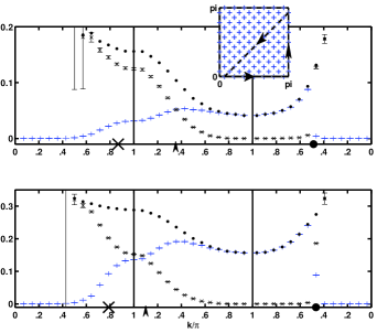
Figure 1: (Color online) QP spectral weights for 6 holes (upper plot, $x\simeq 3\%$) and 22 holes (lower plot, $x\simeq 11\%$) on 196 sites. The spectral weights are plotted along the contour $0\to(0,\pi)\to(\pi,\pi)\to 0$ (shown in inset). Plus signs ($+$, blue online) denote the spectral weight $Z_{\bm{k}}^{+}$, crosses ($\times$) denote $Z_{\bm{k}}^{-}$, error bars are shown. Solid dots (black) denote their sum, the total spectral weight $Z_{\bm{k}}^{tot}$, error bars not shown. On the horizontal axis, the star ($*$) denotes the intersection with the unprojected Fermi surface along the $0\to(0,\pi)$ direction; the thick dot is the nodal point. $Z_{\bm{k}}^{+}$ and $Z_{\bm{k}}^{-}$ jump at the nodal point, while $Z_{\bm{k}}^{tot}$ is continuous. The intersection with the effective Fermi surface (see section V) is marked by an arrowhead. On the diagonal (last segment), $k$ is given in units of $\sqrt{2}$.

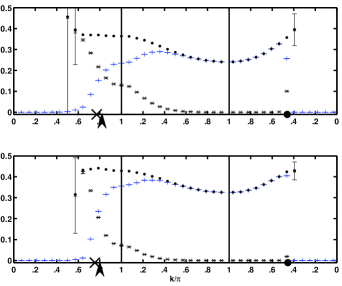
Figure 2: (Color online) Same plot as Fig. 1 of the QP spectral weights for 34 holes (upper plot, $x\simeq 17\%$) and 46 holes (lower plot, $x\simeq 23\%$) on 196 sites.

In Figs. 1 and 2, we plot the spectral weights $Z^{+}_{\bm{k}}$, $Z^{-}_{\bm{k}}$, and $Z^{tot}_{\bm{k}}$ along the contour $0\to(0,\pi)\to(\pi,\pi)\to 0$ in the Brillouin zone for different doping levels. Figure 5 shows the contour plots of $Z^{tot}_{\bm{k}}$ in the region of the Brillouin where our method produces small error bars.note_comp From these data, we can make the following observations:

• In the case of an unprojected BCS wave function, the total spectral weight is constant and unity over the Brillouin zone. Introducing the projection operator, we see that for low doping ($x\simeq 3\%$), the spectral weight is reduced by a factor up to $20$. The renormalization is asymmetric in the sense that the electronic spectral weight $Z^{+}_{\bm{k}}$ is more reduced than the hole spectral weight $Z^{-}_{\bm{k}}$. For higher doping ($x\simeq 23\%$), the spectral weight reduction is much smaller and the electron-hole asymmetry decreases.

• Since there is no electron-hole mixing along the zone diagonal, the spectral weights $Z^{+}_{\bm{k}}$ and $Z^{-}_{\bm{k}}$ have a discontinuity at the nodal point. Our data shows that the total spectral weight is continuous across the nodal point. Strong correlations does not affect this feature of uncorrelated BCS theory. Recently, it has been argued in Ref. yang06, that the total spectral weight of the projected (non-superconducting) Fermi sea should be continuous across the Fermi surface. This is consistent with our result.

The intensities measured in ARPES experiments are proportional to the spectral weights of the low-energy QPs.ARPES In Ref. matsui03, , the spectral weights of a slightly overdoped sample of Bi2223 were measured along the cut $(\pi,0)\rightarrow(\pi/2,\pi/2)$; an almost constant total spectral weight was reported in this experiment. It can be seen from Fig. 5 that the total spectral weight is approximately constant along this cut, so the experimental result agrees with this property of projected wave functions.

An anisotropy of the ARPES intensity along the experimental FS (the so-called nodal-antinodal dichotomy) has been reported in a series of experiments.zhou04 ; shen03 Experimentally, the spectral weight measured in the anti-nodal region is suppressed in underdoped compounds, while it is large in the optimally doped and overdoped region. Usually, this effect is associated with formation of some charge or spin order, static or fluctuating one. From Fig. 5 we see that a similar (but much weaker) tendency can be observed in the framework of Gutzwiller-projected wave functions. The experimentally observed effect is much stronger and a claim that the nodal-antinodal dichotomy can be explained within this framework would be too hasty.

IV Superconducting order parameter

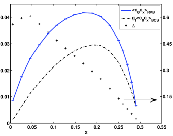
Figure 3: (Color online) Doping dependency of the nearest-neighbor superconducting order parameter $\Phi_{ij}$ (calculated in the 14$\times 14$ system). The error bars are smaller than the symbol size. The same quantity calculated in the Gutzwiller approximation is also shown for comparison. The variational parameter $\Delta$ is shown with the scale on the right.

In Fig. 3, we plot the nearest-neighbor superconducting correlation $\Phi_{ij}$ (the Fourier transform of $\Phi_{\bm{k}}$ defined in (8)) as a function of doping. This curve shows close quantitative agreement with the result of Ref. paramekanti0103, , where the authors extracted the superconducting order parameter from the long range asymptotics of the nearest neighbor pairing correlator, $\lim_{r\rightarrow\infty}\langle c_{0}c_{\delta}c^{\dagger}_{r}c_{r+\delta}^{\dagger}\rangle$. With the method employed here, we find the same qualitative and quantitative conclusions of previous authors:paramekanti0103 ; gros88 vanishing of superconductivity at half filling $x\to 0$ and at the superconducting transition on the overdoped side $x_{c}\simeq 0.3$.note_cc The optimal doping is near $x_{opt}\simeq 0.18$. In the same plot we also show the commonly used Gutzwiller approximation where the BCS order parameter is renormalized by the factor $g_{t}=\frac{2x}{1+x}$.rmft The Gutzwiller approximation underestimates the exact value by approximately $25\%$.

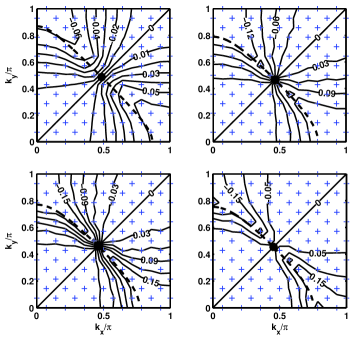
Figure 4: (Color online) Pairing correlation $\Phi_{\bm{k}}$ in the Brillouin Zone at differen doping levels: $x\simeq 3\%$ (upper left), $11\%$ (upper right), $17\%$ (lower left) and $23\%$ (lower right) in a $14\times 14$ system with periodic-antiperiodic boundary conditions. The dashed line is the unprojected FS.

In Fig. 4, we show contour plots of the superconducting order parameter $\Phi_{\bm{k}}$ for four values of doping. It resembles qualitatively the unprojected d-wave pairing amplitude, but is somewhat distorted due to the particle-hole asymmetry (see discussion in the previous and the following sections).

V Fermi surface

In strongly interacting Fermi systems, the notion of a Fermi surface (FS) is not at all clear. There are however several experimental definitions of the FS. Most commonly, ${\bm{k}}_{F}$ is determined in ARPES experiments as the maximum of $|{\bm{\nabla}}_{\bm{k}}n_{\bm{k}}|$ or the locus of minimal gap along some cut in the $\bm{k}$-plane.ARPES The theoretically better defined locus of $n_{\bm{k}}=1/2$ is also sometimes used. The various definitions of the FS usually agree within the experimental uncertainties. Recently, the different definitions of the FS were theoretically analyzed in Refs. gros06,  and sensarma06, .

In our present work, we propose an alternative definition of the Fermi surface based on the ground state equal-time Green’s functions. In the unprojected BCS state, the underlying FS is determined by the condition $|u_{\bm{k}}|^{2}=|v_{\bm{k}}|^{2}$. We will refer to this as the unprojected FS. Since $|u_{\bm{k}}|^{2}$ and $|v_{\bm{k}}|^{2}$ are the residues of the QP poles in the BCS theory, it is natural to replace them in the interacting case by $Z^{+}_{\bm{k}}$ and $Z^{-}_{\bm{k}}$, respectively. We will therefore define the effective FS as the locus $Z^{+}_{\bm{k}}=Z^{-}_{\bm{k}}$.

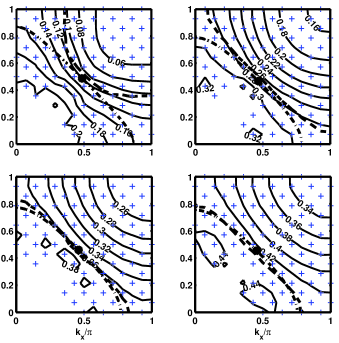
Figure 5: (Color online) Contour plots of the total QP spectral weight $Z_{\bm{k}}^{tot}$. The effective FS (dash line) and unprojected FS (dash-dot line) are also shown. The doping levels are $x\simeq 3\%$ (top left), $11\%$ (top right), $17\%$ (bottom left) and $23\%$ (bottom right). The $+$ signs indicate points where the values are known within small error bars.

In Fig. 5 we plot the unprojected and the effective FS which we obtained from VMC calculations. The contour plot of the total QP weight is also shown. It is interesting to note the following points:

• In the underdoped region, the effective FS is open and bent outwards (hole-like FS). In the overdoped region, the effective FS closes and embraces more and more the unprojected one with increasing doping (electron-like FS).

• Luttinger’s ruleluttinger61 is clearly violated in the underdoped region, i.e. the area enclosed by the effective FS is not conserved by the interaction; it is larger than that of the unprojected one.

• In the optimally doped and overdoped region, the total spectral weight is approximately constant along the effective FS within error bars. In the highly underdoped region, we observe a small concentration of the spectral weight around the nodal point ($\simeq 20\%$).

A large “hole-like” FS in underdoped cuprates has also been reported in ARPES experiments by several groups.ino04 ; yoshida03 ; shen03

It should be noted that a negative next-nearest hopping $t^{\prime}$ would lead to a similar FS curvature as we find in the underdoped region. We would like to emphasize that our original $t$–$J$ Hamiltonian as well as the variational states do not contain any $t^{\prime}$. Our results show that the outward curvature of the FS is due to strong Coulomb repulsion, without need of $t^{\prime}$. The next-nearest hopping terms in the microscopic description of the cuprates may not be necessary to explain the FS topology found in ARPES experiments. Remarkably, if the next-nearest hopping $t^{\prime}$ is included in the variational ansatz (and not in the original $t$–$J$ Hamiltonian), a finite and negative $t^{\prime}$ is generated, as it was shown in Ref. himeda00, . Apparently, in this case the unprojected FS has the tendency to adjust to the effective FS. A similar bending of the FS was also reported in the recent analysis of the current carried by Gutzwiller-projected QPs.nave06 A high-temperature expansion of the momentum distribution function $n_{\bm{k}}$ of the $t$-$J$ model was done in Ref. putikka98, where the authors find a violation of Luttinger’s rule and a negative curvature of the FS. Our findings provide further evidence in this direction.

A natural question is the role of superconductivity in the unconventional bending of the FS. In the limit $\Delta\to 0$, the variational states are Gutzwiller-projected excitations of the Fermi sea and the spectral weights are step-functions at the (unprojected) FS. In a recent paperyang06 it was shown that $\lim_{{\bm{k}}\rightarrow{\bm{k}}^{+}_{F}}Z^{+}_{\bm{k}}=\lim_{{\bm{k}}\rightarrow{\bm{k}}^{-}_{F}}Z^{-}_{\bm{k}}$ for the projected Fermi-sea, which means that the unprojected and the effective FS coincide in that case. This suggests that the “hole-like” FS results from a non-trivial interplay between strong correlation and superconductivity. At the moment, we lack a qualitative explanation of this effect, however it may be a consequence of the proximity of the system to the non-superconducting “staggered-flux” statelee00 ; ivanov03 or to anti-ferromagnetismparamekanti0103 ; ivanov06 near half-filling.

- (1) J. G. Bednorz and K. A. Müller, Z. Phys. B 64, 189 (1986).
- (2) P. W. Anderson, Science 235, 1196 (1987).
- (3) C. Gros, Phys. Rev. B 38, 931 (1988); C. Gros, Ann. Phys 189, 53 (1989).
- (4) H. Yokoyama and H. Shiba, J. Phys. Soc. Jpn. 57, 2482 (1988).
- (5) Y. Hasegawa and D. Poilblanc, Phys. Rev. B 40, 9035 (1989).
- (6) F. Becca, L. Capriotti, and S. Sorella, cond-mat/0006353.
- (7) A. Paramekanti, M. Randeria, and N. Trivedi, Phys. Rev. Lett. 87, 217002 (2001); A. Paramekanti, M. Randeria, and N. Trivedi, Phys. Rev. B 70, 054504 (2004); M. Randeria, R. Sensarma, N. Tirvedi, and F.-Ch. Zhang, Phys. Ref. Lett. 95, 137001 (2005).
- (8) F. C. Zhang, C. Gros, T. M. Rice and H. Shiba, Sup. Sci. Tech. 1, 36 (1988); P. W. Anderson, P. A. Lee, M. Randeria, M. Rice, N. Trivedi and F. C. Zhang, J. Phys. Cond. Mat. 16, R755 (2004).
- (9) A. Damascelli, Z. Hussain, and Z.-X. Shen, Rev. Mod. Phys. 75, 473 (2003); J. C. Campuzano, M. R. Norman, and M. Randeria, cond-mat/0209476.
- (10) H. Matsui, T. Sato, T. Takahashi, S.-C. Wang, H.-B. Yang, H. Ding, T. Fujii, T. Watanabe, and A. Matsuda, Phys. Rev. Lett. 90, 217002 (2003).
- (11) S. Yunoki, Phy. Rev. B 72, 092505 (2005).
- (12) S. Yunoki, E. Dagotto, and S. Sorella, Phys. Rev. Lett. 94, 037001 (2005).
- (13) B. Edegger, V. N. Muthukumar, C. Gros, and P. W. Anderson, Phys. Rev. Lett. 96, 207002 (2006).
- (14) C. P. Nave, D. A. Ivanov, and P. A. Lee, Phys. Rev. B 73, 104502 (2006).
- (15) C. Gros, R. Joynt, and T. M. Rice, Phys. Rev. B 36, 381 (1978).
- (16) J. M. Luttinger, Phys. Rev. 121, 942 (1961).
- (17) C. Gros, B. Edegger, V. N. Muthukumar, and P. W. Anderson, cond-mat/0606750.
- (18) R. Sensarma, M. Randeria, and N. Trivedi, cond-mat/0607006.
- (19) P. Fazekas, Lecture notes on electron correlation and magnetism (World Scientific, 1999).
- (20) F. C. Zhang and T. M. Rice, Phys. Rev. B, 37, 3759 (1988).
- (21) D. A. Ivanov and P. A. Lee, Phys. Rev. B 68, 132501 (2003).
- (22) D. Poilblanc, J. Riera, and E. Dagotto, Phys. Rev. B 49, 12318 (1994).
- (23) K. Park, Phys. Rev. B 72, 245116 (2005).
- (24) Y. Ohta, T. Shimozato, R. Eder, and S. Maekawa, Phys. Rev. Lett. 73, 324 (1994).
- (25) S. Yunoki, private communication (2006).
- (26) H. Yang, F. Yang, Y.-J. Jiang, and T. Li, cond-mat/0604488.
- (27) K. M. Shen, F. Ronning, D. H. Lu, F. Baumberger, N. J. C. Ingle, W. S. Lee, W. Meevasana, Y. Kohsaka, M. Azuma, M. Takano, and Z.-X. Shen, Science 307, 901 (2005).
- (28) X. J. Zhou, T. Yoshida, A. Lanzara, P. V. Bogdanov, S. A. Kellar, K. M. Shen, W. L. Yang, F. Ronning, T. Sasagawa, T. Kakeshita, T. Noda, H. Eisaki, S. Uchida, C. T. Lin, F. Zhou, J. W. Xiong, W. X. Ti, Z. X. Zhao, A. Fujimori, Z. Hussain, and Z.-X. Shen, Phys. Rev. Lett. 92, 187001 (2004).
- (29) A. Ino, C. Kim, M. Nakamura, T. Yoshida, T. Mizokawa, A. Fujimori, Z.-X. Shen, T. Kakeshita, H. Eisaki, and S. Uchida, Phys. Rev. B 65, 094504 (2002).
- (30) T. Yoshida, X. J. Zhou, T. Sasagawa, W. L. Yang, P. V. Bogdanov, A. Lanzara, Z. Hussain, T. Mizokawa, A. Fujimori, H. Eisaki, Z.-X. Shen, T. Kakeshita, and S. Uchida, Phys. Rev. Lett. 91, 027001 (2003).
- (31) A. Himeda and M. Ogata, Phys. Rev. Lett. 85, 4345 (2000).
- (32) W. O. Putikka, M. U. Luchini, and R. R. P. Singh, Phys. Rev. Lett. 81, 2966 (1998).
- (33) P. A. Lee and X.-G. Wen, Phys. Rev. B 63, 224517 (2000).
- (34) D. A. Ivanov, Phys. Rev. B 74, 24525 (2006).
- (35) Ch. P. Chou, T. K. Lee, and Ch.-M. Ho, cond-mat/0606633.
- (36) B. Edegger, N. Fukushima, C. Gros, and V. N. Muthukumar, Phys. Rev. B 72 134504 (2005).
- (37) As an alternative to the micro-canonical formulation in Eqs. (2) and (3), one can work in the grand-canonical ensemble, without the particle-number projector, but with an additional fugacity factor.edegger05 In this paper, the micro-canonical scheme is chosen for numerical convenience, as it is commonly done in most VMC studies.
- (38) It is interesting to note that we observe a relatively sensitive dependency of the superconducting order parameter on the variational parameter at high doping (as ). This results from projecting the particle-number tail of an almost normal state (), if the value of is far away from the Fermi-sea chemical potential. Remarkably, the variational value of approaches the Fermi-sea chemical potential as .ivanov03 In the projected Fermi-sea, can no longer be treated as a variational parameter, but is fixed by the particle-number constraint. (The variational must not be confused with the chemical potential.)
- (39) Our VMC results show good agreement with the hole spectral weight reported in Ref. edegger06, where the authors used an extended Gutzwiller approximation to calculate the same quantity in the large-U Hubbard model. It should be noted, however, that the asymmetry found in the present paper cannot be explained within any known Gutzwiller approximation scheme. Our results are consistent with other recent VMC calculationsnave06 ; yang06 ; yunoki06 and earlier calculations of in Ref. paramekanti0103, .