SLAC-PUB-12039 August 1, 2006 Exploring Contractor Renormalization: Tests on the 2-D Heisenberg Antiferromagnet and Some New Perspectives

Abstract

Contractor Renormalization (CORE) is a numerical renormalization method for Hamiltonian systems that has found applications in particle and condensed matter physics. There have been few studies, however, on further understanding of what exactly it does and its convergence properties. The current work has two main objectives. First, we wish to investigate the convergence of the cluster expansion for a two-dimensional Heisenberg Antiferromagnet(HAF). This is important because the linked cluster expansion used to evaluate this formula non-perturbatively is not controlled by a small parameter. Here we present a study of three different blocking schemes which reveals some surprises and in particular, leads us to suggest a scheme for defining successive terms in the cluster expansion. Our second goal is to present some new perspectives on CORE in light of recent developments to make it accessible to more researchers, including those in Quantum Information Science. We make some comparison to entanglement-based approaches and discuss how it may be possible to improve or generalize the method.

I 1. Introduction and Outline

Many problems in physics, in areas ranging from particle and condensed matter physics to theoretical quantum computing, can only be treated by numerical methods. Among them is the particularly interesting problem of extracting the low energy behavior of a multi-dimensional system defined by a Hamiltonian with local interactions. While analytical methods can be applied to a few such Hamiltonians, existing methods generally require enormous computational power to study systems of even modest size. For example, Quantum Monte Carlo can give highly accurate results for many systems, but its applicability can be limited by the fermion sign problem, as well as the inaccuracies inherent in extrapolating finite size results to the limit of infinite volume. The most popular alternative, the Density Matrix Renormalization Group method (DMRG)densitymatrix , is particularly successful in one dimension. With the advent of Quantum Information Science, it has been extended to simulate time evolution TEBD and multidimensional models (PEPS or tensor networksPEPS ; TN ). The idea underlying DMRG and its generalizations is a clever variational ansatz - the representation of states as contracted tensors. This approach has many virtues. For example, it provides an upper bound on the ground state energy density. One can also extract quantities such as total entropy which is approximately preserved in the subspace and use them to analyze phase transition LegezaPT ; Latorre . It has its limitations, however, as one has to deal with convergence issues and a very large number of states in more complicated systems. The closely-related method described in PEPS also has the requirement of a fixed finite lattice.

In search for an alternative method, one might reasonably ask if there is a way that encodes the information about the ground state and low lying excited states not in states, but in operators . One method that does that is the Contractor Renormalization Group Method (CORE)COREpaper , which, like DMRG, is an attempt to improve Wilson’s real-space renormalizationWilson . Similar ideas have appeared in the past Cloizeaux ; Zivkovic but we will follow the terminology of COREpaper as it is the first general formulation of the method. (The same formulation was also independently proposed as Real-Space Renormalization Group with Effective Interaction (RSRG-EI) in MalrieuGuihery ). While the method has intuitive appeal and has been used to study many collective phenomenaCOREpaper2 ; calzado ; somepapers , unlike in the case of DMRG, we have relatively little grasp of exactly why and when the algorithm works. There seems to be a need to put aside applications for a moment and look at the method more closely. Short of very conclusive results, we present here some findings that may lead to a better understanding of CORE. We approach the issue from two angles. First, we take the simplest 2-D model as a testing ground and carry out successive numerical renormalization using three different blocking schemes. Our choice, the Heisenberg Antiferromagnet (HAF), has been studied with RSRG-EI in the past MalrieuGuihery , but our focus is on the extraction of order parameter and the behavior of long-range operators in the 2-D cluster expansion, particularly because there is a freedom in defining successive terms in the expansion LegezaOrder . We also look at how well different blocking schemes agree with each other while capturing the physics in distinct ways. Secondly, we make some theoretical and numerical comparison between CORE and DMRG as well as Entanglement Renormalization DU . By presenting a slightly different perspective, we hope to provoke further investigation into the limitations of the method and the possibility for improvement.

Section 2 of the paper reviews the basic formulas in CORE and sets the notation. The first subsection of Section 3 presents calculation of CORE on nine-site blocks, as considered in MalrieuGuihery . In addition to the energy density, which can be easily obtained to high accuracy, we calculate the staggered magnetization and find that, without longer-range operators, it is only accurate to one significant figure. To see how longer-range terms behave with limited computing resource, we use smaller blocks in section 3(b) (four-site) and 3(c) (five-site) and compute the energy density. We find that operators beyond nearest-neighbor can contribute quite significantly and requires very careful ordering. To this end we propose a ordering scheme based on diameters of the clusters. The effect of long-range operator, however, does not necessarily correspond to long-range correlation, as we see in 3(b) that even with only nearest neighbor operators a vanishing mass gap appears non-trivially. Although application is not the focus of the current work, we also show as a side note in Section 3(c) how, under the appropriate blocking, CORE might provide an interesting justification for the spin-wave approximation.

In Section 4 we turn to the question of how CORE relates to entanglement-based approaches. In the first subsection we discuss truncation and blocking schemes of CORE and DMRG and compare their principles. We show that for a small, finite toy model CORE yields results comparable to DMRG. Then in Section 4(b) we formulate CORE in a way that enables us to see its similarity to Entanglement RenormalizationDU , which should be more familiar to readers in Quantum Information Science. We also discuss in Section 4(c) the role of block entropy in CORE and its possible use. Finally in Section 4(d) we discuss how the choice of retained states in CORE can affect its performance and what entanglement has to do with this choice.

In Section 5 we reprise our results and discuss a number of future directions and possibilities.

II 2. CORE: The Basic Formulas

The original description of CORE can be found in Ref.COREpaper . This section summarizes the basic formulas we will use in the sections to follow (particularly in Section 4).

Given a Hamiltonian $H$ on Hilbert space $\cal H$, the renormalized Hamiltonian that CORE seeks to approximate takes the form:

$$H_{ren}(t) =$$

$$\hskip-35.0pt(Pe^{-2Ht}P)^{-\frac{1}{2}}Pe^{-Ht}He^{-Ht}P(Pe^{-2Ht}P)^{-\frac{1}{2}}.$$

where $P$ is a projection operator from $\cal H$ onto $\cal H^{\prime}$, a chosen subspace of retained states (in the language of RSRG-EIMalrieuGuihery , the model space). $t$ is a variable parameter usually taken to infinity. With the following lemma, we can show that $H_{ren}=\lim_{t\to\infty}H_{ren}(t)$ takes a particularly simple form.

Lemma 1

Let $\left|{a_{i}}\right\rangle,i=1,\ldots,M$ be an arbitrary orthonormal basis for ${\cal H^{\prime}}$ and let $\left|{v_{l}}\right\rangle,l=1,\ldots,N$, be an orthonormal set of eigenvectors of the Hamiltonian, $H$, with eigenvalues $\{E_{1},E_{2},\ldots,E_{l}\ldots\}$ arranged in ascending order (generally, $M<N$). Then, there exists an $M\times M$ matrix, $R_{ij}$, such that the states $\left|{w_{j}}\right\rangle=\sum_{i=1}^{M}R_{ij}\left|{a_{i}}\right\rangle$ have the property that for each $j$, there is exactly one index $1\leq f(j)\leq N$ such that $\left\langle{w_{j}}|{v_{f(j)}}\right\rangle\neq 0$ and $\left\langle{w_{k}}|{v_{f(j)}}\right\rangle=0\,\forall k>j$.

Corollary 1

Each state $\left|{w_{j}}\right\rangle$ has the property that

$$e^{-Ht}\left|{w_{j}}\right\rangle\sim_{t\to\infty}e^{-E_{f(j)}t}\left\langle{v_{f(j)}}|{w_{j}}\right\rangle\left|{v_{f(j)}}\right\rangle+\ldots,$$ (2)

where $\ldots$ stands for terms that vanish more rapidly as $t\to\infty$.

Then it can be proved that:

$$H_{ren} = \sum_{i,j,k}\left|{a_{j}}\right\rangle R^{{\dagger}}_{ji}E_{f(i)}R_{ik}\left\langle{a_{k}}\right|,$$ (3)

$$= \sum_{i}\left|{w_{i}}\right\rangle E_{f(i)}\left\langle{w_{i}}\right|.$$

On a lattice we may expand this renormalized Hamiltonian as linked clusters:

$$H_{ren}=\sum_{s\subset L}h^{conn}(s),$$

$$h^{conn}(s)\equiv H_{ren}\mid_{s}-\sum_{s^{\prime}\subset s}h^{conn}(s^{\prime})$$ (4)

where $L$ is the entire lattice corresponding to $\cal H^{\prime}$ (it can be infinite) and $s$ is a connected sublattice. $H_{ren}\mid_{s}$ is $H_{ren}$ evaluated for the theory obtained by restricting the full Hamiltonian to the sublattice $s$. For notational convenience, operators acting on $s$ are implicitly assumed to extend to the full lattice by acting as the identity operator on degrees of freedom lying outside of $s$. We will also refer to $h^{conn}(s)$ as a range-$r$ connected operator if $s$ contains $r$ blocks used to define the projection $P$, and we will adopt the notation $h^{conn}(s^{r})$ to denote such an operator.

In practice we can of course only evaluate range-$r$ operators for small $r$, but since the longer-range terms are not controlled by a small parameter (this would be true if $t$ is a small number), we would have to be careful what to discard and we will discuss some examples in the next section.

III 3. The Two-Dimensional Heisenberg Antiferromagnet

We have chosen the 2-D spin-1/2 HAF as testing ground for its simplicity and connection to the Hubbard model. The Hamiltonian is defined as

$$H = \sum_{<i,j>}\vec{S}_{i}\cdot\vec{S}_{j}$$ (5)

$$= \sum_{<i,j>}S^{x}_{i}\cdot S^{x}_{j}+S^{y}_{i}\cdot S^{y}_{j}+S^{z}_{i}\cdot S^{z}_{j},$$

where the sum is over all neighboring pairs on a two-dimensional square lattice.

III.1 a. Nine-site Square Blocking

Although we are not able to compute (on a PC) long-range terms with nine-site blocks, their simplicity allows us to see some basic features of the computation and the HAF we are studying. The nine-site block is a natural extension of the three-site block in 1-D COREpaper as it also has a spin-1/2 multiplet as ground states which we use as retained states. The range-1 and range-2 operators take the form:

$$h^{conn}(s^{1})=\alpha_{0}\mathbf{1}$$

$$h^{conn}(s^{2})=\alpha_{1}\mathbf{1}+\beta_{1}\vec{S}\cdot\vec{S}.$$ (6)

where we denote the one-block and two-adjacent-block configurations by $s^{1}$ and $s^{2}$ respectively. Note that no calculation of $R$ in Eq.1 is necessary to find $h^{conn}(s^{2})$, because the retained states form exactly a spin-0 multiplet and spin-1 multiplet. If we are to preserve the spin symmetry, there are no other inequivalent rotations. The fact that spin symmetry largely dictates possible eigenvectors of the renormalized Hamiltonian greatly reduces computational effort, though arguably, we can only test the effect of CORE’s recipe for $R$ in more complicated situations where there are many multiplets of the same spin. (From our experience it is also possible to break the spin symmetry and let CORE decide the best linear combination. This often yields a good ground state energy but a poor spectral distribution.)

With the range-1 and range-2 operators above, we can easily calculate the ground state energy density by summing a geometric series and reproduce the result of Zivkovic ; MalrieuGuihery . The energy per site obtained this way is $-0.666$ and within $0.5\%$ of the Monte Carlo result $-0.669$exact . The situation becomes much more complicated, however, when we we proceed to calculate the staggered magnetization, an order parameter of the HAF. There are two ways of calculating the expectation value of a renormalized operator. In COREpaper it is argued that other operators should take a form similar to Eq.3:

$$O_{ren}=R^{\dagger}OR,$$ (7)

where now $O$ is the matrix in the $\left|{w_{i}}\right\rangle$ basis

$$O_{ij}=\left\langle{w_{i}}\right|O\left|{w_{j}}\right\rangle.$$ (8)

But since the staggered magnetization does not easily converge to a simple form as the Hamiltonian does, it is easier to calculate the expectation value by:

$${\langle O\rangle}=\frac{\delta\langle H+JO\rangle}{\delta J}\mid_{J=0}$$ (9)

. In other words, we add a multiple of the staggered magnetization operator, $JM_{stag}$, to the Hamiltonian, use CORE to compute the ground state energy density, $E(J)$, and extract the slope of this function at $J=0$(see Eq.9). Once we have added $JM_{stag}$ to the starting Hamiltonian the renormalized Hamiltonian is no longer a simple multiple of the original Hamiltonian and obtaining $E(J)$ requires running the RG until it converges. In Fig.1 we plot the ground state energy obtained in this way as a function of $J$. The staggered magnetization is the slope of the curve at $J=0$ and is obtained by fitting to a fourth-order polynomial in $J$.

Figure 1: A plot of staggered magnetic field J vs energy density E. Staggered magnetization can be calculated from $\langle M\rangle=\frac{\delta\langle H+JM\rangle}{\delta J}\mid_{J=0}$. The data points have to be close enough to see the curvature but sparse enough so that error in the energy will not affect the slope between the points too significantly.

How small can we set the $J$-values to be? If we are allowed to use the knowledge that the energy obtained is accurate to two significant figures, we have to choose the $J$-values to be large enough so that the error in the slope will be at least one order of magnitude smaller than the slope itself. The expectation value thus obtained is $M_{stag}=-0.29$, whereas the exact Monte Carlo result is $-0.30$exact . We must caution though that if we use smaller $J$’s or change the order of the polynomial fit, we can change the result by up to $20\%$. To calculate the order parameter more reliably, it seems that one has to find a way to capture more physical information in the renormalization.

III.2 b. Four-site Square blocking

In the case of the four-site block the lowest lying states form a spin-0 singlet and a spin-1 triplet. In this case, the renormalized Hamiltonian is no longer isomorphic, even at range-2, to the original Hamiltonian which had a single spin-1/2 degree of freedom associated with each site. Furthermore, it appears to describe a theory with a non-vanishing mass gap, as subsequent RG-steps continues to have a spin-0 and a spin-1 multiplet as its lowest energy eigenstates. This single-site gap, however, is just a reflection of the uncertainty principle cost one must pay for localizing the spin-1 excitation to a single block. By keeping these two multiplets at every step, we run the RG until the energy density converges and find that the gap between the two multiplets converges to zero. This reflects the fact that spin-1/2 HAF is massless and agrees with the result of nine-site and five-site blockings, where the ground state is by contruction degenerate. We would like to note that this result is entirely non-trivial, since the original Wilsonian RSRG (the $t=0$ limit of the CORE formula for the renormalized Hamiltonian) predicts that the same theory dimerizes and has a non-vanishing mass gap.

While this result gives us some confidence that even the lowest order cluster expansion is doing fairly well at extracting the correct physics, we obtain $-0.710$ for the ground state energy density - it is not nearly as accurate as the nine-site case. This is perhaps to be expected given that we have exactly diagonalized a mere $256$ states here (whereas we have diagonalized $2^{18}$ states in the nine-site calculation), yet in some sense it is still remarkable, since we have kept proportionally more states in every iteration (4-out-of-16 vs 2-out-of-512). To check the convergence of the cluster expansion, we add the operator corresponding to a sub-cluster consisting of four blocks arranged in a square. We do this only for the first RG step as the analogous term in the next iteration requires diagonalization of $2^{32}$ states. This already improves the energy density to $-0.677$ and allows us to obtain a staggered magnetization that is close to the nine-site case. At this point we might be prompted to ask: To achieve a good accuracy, do we simply compute all the terms within our computational power? Since the five-site blocking exhibits the most numerical sensitivity to the ordering in the cluster expansion, we defer a more detailed discussion to the next subsection.

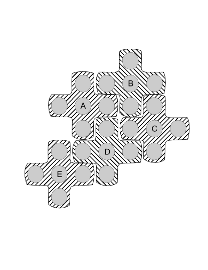
Figure 2: Blocking of five-site stars. A total of five blocks are shown in the figure. range-2 terms are connected operators on two adajcent blocks, such as A and B. There are two types of range-3 terms: Examples of ”L”s include ABC, BCD, etc., while there is a straight-line term on CDE. Finally, the range-4 plaquette acts on ABCD.

III.3 c. Five-site Star blocking

The final CORE computation we wish to discuss uses the five-site blocks shown in Fig.2. What makes the RG transformation following from this blocking procedure interesting is that it behaves quite differently from the one obtained by restricting attention to square blocks. This is because the ground state of a star, in contrast to the nine-site block, is a spin-3/2 multiplet. The renormalized Hamiltonian at range two takes the general form

$$h^{conn}(s^{2})=c_{0}\mathbf{1}+c_{1}\vec{S}\cdot\vec{S}+c_{2}(\vec{S}\cdot\vec{S})^{2}+c_{3}(\vec{S}\cdot\vec{S})^{3}.$$ (10)

If we evaluate the expectation value of Eq.10 in the classical Néel state, we obtain an upper bound on the energy density of -0.712 per site. So despite the fact that the fundamental block has more sites, this accuracy is worse than the equivalent four-site blocking. Notice that the ratio of intra-block over inter-block links is smaller with five-site blocks. We suspect that the large perimeter of star blocks result in many under-constrained sites near the edge of the configuration.

Nevertheless, we can continue to run the renormalization group to see how the theory changes. If we use the Hamiltonian defined in Eq.10 and once again calculate the spectrum of a single star we find that now the ground state is a spin-9/2 multiplet. Keeping the spin-9/2 multiplets as new degrees of freedom, we find that the range-2 interaction again to be antiferromagnetic. We use these interactions to construct a five-site star, and the ground state now becomes a spin-$27/2$ multiplet. From this version of CORE we see that the spin-$1/2$ theory is equivalent to a theory with a larger spin at each site.

Clearly the stability of a picture that says that spins keep growing with each renormalization group step must be checked by computing the contributions to the renormalized Hamiltonian coming from larger clusters. The reason this is interesting is that once one goes to larger sub-clusters, one introduces new diagonal couplings, couplings involving three sites at a time, etc. Since the diagonal couplings are also mainly antiferromagnetic in character, they tend to introduce frustration into the system. It is entirely possible that these are relevant operators and significantly modify the nature of the RG flow, so that at the next step the spins fail to grow.

To obtain a qualitative understanding of how each connected operator modifies the flow of the renormalized Hamiltonian we first observe that each three-site connected operator can be written as a sum of terms which act non-trivially on one, two or three-sites at a time. To see why this is true let us assume that we have spin-$n/2$ on each site of the new lattice and let $X_{i},i=2..n+1$ be a set of $n$ traceless matrices which, together with the matrix $X_{1}=1/(n+1)\,{\bf 1}$ (where ${\bf 1}$ is the unit matrix), form a basis for the space of of $(n+1)\times(n+1)$ matrices. Furthermore, assume that these matrices satisfy the normalization conditions

$${\rm Tr}(X_{i}\,X_{j})=\delta_{ij}.$$ (11)

It then follows that the tensor products

$$M_{ijk}=X_{i}\otimes X_{j}\otimes X_{j}$$ (12)

form a normalized basis of matrices which operate on three lattice sites at a time. Thus, the general three-site connected operator can be written as

$$O=\sum_{i,j,k}\alpha_{ijk}M_{ijk}.$$ (13)

Furthermore, the coefficents $\alpha_{ijk}$ can be extracted by taking the trace with any $M_{ijk}$; i.e.,

$$\alpha_{ijk}={\rm Tr}(M_{ijk}O).$$ (14)

Given this definition, it is easy to define what we mean by the parts of $O$ which act non-trivially on zero, one, two or all three sites. The part of $O$ that is proportional to a multiple of the unit matrix is, of course, a term that acts trivially on all three sites and won’t contribute to dynamics. Of what remains, it typically turns out that the operators which act non-trivially on only one or two sites are the most important operators. Thus, for the purpose of getting a simple qualitative understanding of the stability of our problem we restrict attention to these operators in what follows. Since the renormalized Hamiltonian must commute with the total spin operator, it follows from direct computation, or simple group theory, that there are no terms in the renormalized Hamiltonian which act non-trivially on a single block. (This is because for spin-$n/2$, the space of $(2n+1)\times(2n+1)$ matrices decomposes, under total spin, into matrices which transform as spin-$0$, the unit matrix, and, for each $j$, a set of matrices which transform as spin-$j$, where $j$ runs from $1\ldots 2n+1$.) Similar arguments tell us that operators that act non-trivially on only two-sites at a time can be written as polynomials in $\vec{S}\cdot\vec{S}$ acting on the two-sites in question. By $\vec{S}$ we mean the matrices which represent the generators of spin rotations for spin-$n/2$. Note, the order of the polynomial for the case of spin-$n/2$ is at most $2n$.

Having said this we can ask what the effects of the terms proportional $\vec{S}\cdot\vec{S}$ (which act on only two-sites at a time) coming from the straight line, the L and the plaquette are (this terminology is best explained by looking at Fig.2.), since these two-site operators turn out to be a significant part of the contribution to the renormalized Hamiltonian. There are three important observations that we must make about these terms.

First, the antiferromagnetic interaction between diagonal sites (e.g., BD in Fig.2) are of the same order of magnitude as the interaction between adjacent sites. This means that the contribution of larger clusters to the renormalization group transformation generically produce a frustrated system. Second, unlike the case of one dimension, where the importance of operators coming from larger clusters falls off with the number of blocks in a cluster, terms coming from the four-block plaquette appear to be as important as those coming from clusters consisting of only three-blocks. (Among the three types of terms we evaluated, the three-block straight-line has the smallest two-site contributions.) Third, the two-site terms coming from different clusters often cancel each other, indicating that our result is sensitive to how we define the cluster expansion. To give the reader a feeling for these three points we include the following table which shows how the energy density changes with the inclusion of different terms when we approximate the ground state with the Neel state at the spin-3/2 level.

Terms included	Approx. energy density
Only range-2	-0.712
+”L”	-0.623
+”L”+”line”	-0.586
+”L”+plaquette	-0.637
+”L”+”line”+plaquette	-0.600

At this point it is natural to ask, “What is the best way to arrange the terms in the cluster expansion?”. Intuitively, we expect the contribution of a long chain in a straight line to be less than the contribution of a square with the same number of blocks, because the blocks in the latter case are closer to each other. Taking this with the observations above, we propose a cluster re-summation that treats all clusters having the same diameter as having equal weight. By the diameter of a cluster we mean the longest distance between two blocks in the configuration. For example, the diameter for the range-2 term would be one, for the three-block ”L” and four-block plaquette term $\sqrt{2}$, etc. This scheme has the additional advantage that now each term in the cluster expansion preserves at least some of the rotational symmetry of the lattice since, at every order, we include all the terms with the same diameter.

Note that in a diameter expansion the four-block plaquette comes before the three-block straight-line, which has diameter two. Of course, to be sure that all terms coming from clusters of diameter $2$ are smaller than those of diameter $1$ and diameter $\sqrt{2}$, we should have also evaluated the cluster where four blocks are arranged in a ”T”. We left it out because, for symmetry reasons, this configuration is considerably more difficult to evaluate than the plaquette and we wanted to limit this study to computations easily carried out on an average personal computer. Using only the plaquette and ”L” terms, the ground state of the five-site spin-3/2 star again turns out to be a spin-9/2 multiplet. This is somewhat remarkable. Even with pure $\vec{S}\cdot\vec{S}$ type interactions between adjacent and diagonal sites, the ground state of the generically frustrated five-site star could have been spin-1/2, spin-3/2 or spin-9/2 depending on relative strengths of the interactions.

In principle we should now proceed to calculate the interactions for the spin-9/2 theory up to the same diameter. Unfortunately, calculations of the plaquette in the spin-9/2 theory requires the diagonalization of a sparse $4^{20}\times 4^{20}$ matrix, so we are restricted to range-2 (diameter-1) as in the four-site case. The range-2 interaction remains antiferromagnetic but by itself gives an energy density that is less than $-0.78$.

Although, due to limited resources, we do not have the longer range terms to show a converging result, we would like to close this discussion by noting that this is very interesting in the context of the spin-wave approximation to the HAF. Since turning the spins into Holstein-Primakoff bosons rely on an expansion in $1/2S$, a validated picture of growing spin essentially explains the well-known accuracy of the spin-wave method on the spin-1/2 lattice. We can estimate the error in the $1/2S$ expansion for a finite spin-9/2 lattice. We take our range-2-only calculation and rewrite the Hamiltonian on one five-site block of spin-9/2 using Holstein-Primakoff bosons, keeping only oscillator terms that are of no higher power than the number operator. We then find the ground state energy by minimizing over Bogoliubov transformation parameters. The value calculated this way differs only by $0.02\%$ from the exact energy of the spin-27/2 multiplet.

In conclusion, the three-blocking schemes give us three different physical pictures for the same system. The sensitivity of CORE to link structures suggests that, when working with exotic blocking schemes, one has to check very carefully the convergence of the cluster expansion. Moreover, our experimentation with various ways of resumming range-3 and range-4 terms indicates that the RG-flow can be changed dramatically depending on how we group and order the operators in the cluster expansion. The diameter expansion we proposed appears to be the most plausible solution, but in absence of rigorous theorems bounding the long-range terms, this remains an open problem.

IV 4. Comparison to Entanglement-based Approaches

IV.1 a. Density Matrix Renormalization

The remainder of this paper is devoted to comparing CORE to other methods in a way we hope would shed light on the features of CORE. Given the popularity of DMRG, we take it as an instructive benchmark for studying CORE’s performance. This sort of comparison has not been made in the past because the two methods in their respective original formulations have very different blocking and truncation schemes and it seemed difficult to compare them in a meaningful way. There are two essential features in the original formulation of DMRG (we refer the readers to Refs.densitymatrix for details):

• Reduced Density Matrix Truncation - In each block we select what to keep according to the reduced density matrix of a target state, usually the ground state of a larger system. The larger system is the block whose truncation we are interested in plus an ”environment”, which can be for example a copy of the block. Truncation consists of eliminating those vectors with the smallest eigenvalues of the reduced density matrix obtained by tracing out the environment. The error in the truncation depends on the distribution of eigenvalues of the reduced density matrix and can be analyzed in the language of quantum data compressionLegezaEnt .
  

• Linear Blocking - The block size increases linearly one site at a time. This naturally allows iterative improvement by back and forth sweeps and gives rise to the underlying matrix product state structure. Yet this is not renormalization in the sense of coarse-graining one theory to another of a different scale. To do so one could, of course, use hierarchical blocking (Fig.3A) along with the reduced density matrix truncation described in I (We will refer to this as ”Hierarchical DMRG” or HDMRG), but it is usually not preferred. Roughly speaking, the reason is that entanglement often scales with the boundary of the block, and because hierarchical blocking gives rise to more boundaries, truncation in HDMRG results in more loss of information.

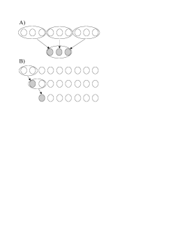
Figure 3: A) Hierarchical Blocking allows renormalization in the Wilsonian sense. B) Linear Blocking instead grows the block by one site at a time and works better for the original DMRG. (Details about the environment omitted above.)

CORE as formulated in Section 2 does not rely on specific truncation and blocking schemes - they are details of the projection operator $P$. The scheme we use in Section 3 can be classified as ”hierarchical blocking” (Fig.3A) and we will refer to it as such. (Though unlike HDMRG or naive real-space renormalization, the state cannot be reconstructed in the original space in a simple hierarchical manner.)

Since we are free are to choose the form of the projection operator, this difference between CORE and DMRG can be considered a superficial one. As we mentioned in the Introduction, the essential feature of CORE is that it encodes some information in operators instead of states. To see this in a formulation that allows direct comparison, let us consider the alternative form of DMRG - the matrix product states (MPS) formalism. One common way to obtain the ground state energy using MPS is by applying an imaginary time evolution to a simple starting state, which we will call $\left|{\psi}\right\rangle$. Suzuki-Trotter decomposition can be used to decompose the evolution into small steps and after every step the state will be truncated to make sure that it lies within the subspace spanned by MPS of a fixed dimension. If the procedure converges successfully to the desired attractor and $P$ is a projection onto the MPS subspace, the final state should be the same as $Pe^{-Ht}\left|{\psi}\right\rangle=Pe^{-Ht}P\left|{\psi}\right\rangle$ where $t$ is taken to infinity and the equality follows from the fact that the starting state lies within the projected subspace. The ground state energy is therefore:

$$E_{0}=\frac{\left\langle{\psi}\right|Pe^{-Ht}PHPe^{-Ht}P\left|{\psi}\right\rangle}{\left\langle{\psi}\right|Pe^{-Ht}Pe^{-Ht}P\left|{\psi}\right\rangle}$$ (15)

This means $E_{0}$ is the smallest eigenvalue of the Hamiltonian:

$$H^{\prime}_{ren}(t)=$$

$$(Pe^{-Ht}Pe^{-Ht}P)^{-\frac{1}{2}}Pe^{-Ht}PHPe^{-Ht}P(Pe^{-Ht}Pe^{-Ht}P)^{-\frac{1}{2}}$$

We can now contrast this directly with Eq.LABEL:Hrent. $H_{ren}(t)$ in Eq.LABEL:Hrent contains the exact ground state energy but cannot be evaluated exactly, therefore we have to throw away the long-range terms caused by the diffusion of $e^{-Ht}$. When the additional projections are inserted in $H^{\prime}_{ren}(t)$ of Eq.LABEL:HrenMPS, it no longer contains the exact ground state energy, but its ground state energy can be found exactly. In this case the burden of a good approximation is shifted entirely to a clever choice of $P$.

Having seen an abstract comparison, let us now return to the original form of DMRG and compare some numbers. Because hierarchical blocking allows CORE to handle very large lattices and DMRG requires linear blocking, one might expect CORE’s strength to be with large systems. We were surprised to find, however, that even on small finite lattices, CORE achieves accuracies that are comparable to DMRG. We demonstrate this by running HDMRG, DMRG and CORE on a short periodic Ising chain.

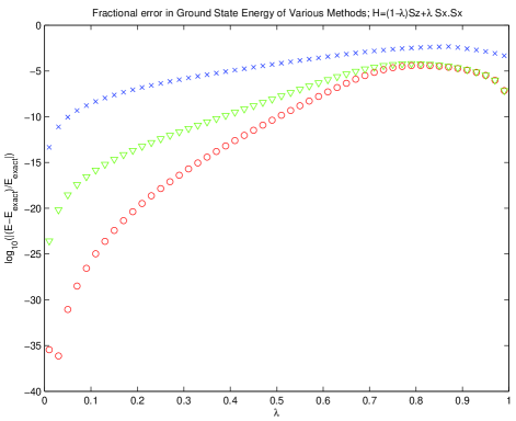
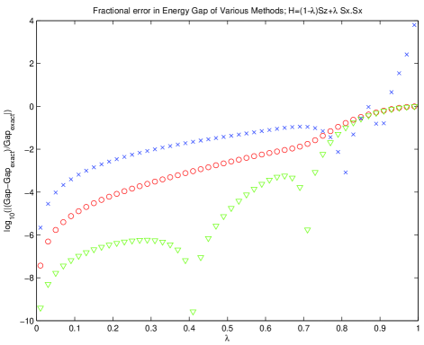
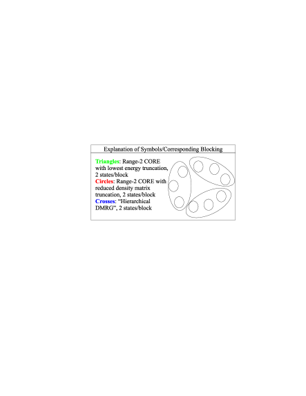
Figure 4: Performance of various methods on a nine-site periodic Ising system. The two CORE cases (triangles and circles) use different truncation schemes. One keeps the lowest energy states within the block; another finds the ground state of two blocks and considers its reduced density matrix. They are compared to HDMRG with the same blocking scheme.

The first set of plots, Fig.4, is for the nine-site periodic Ising chain and compares CORE to HDMRG. This is an interesting comparison since we can naturally use hierarchical blocking for both. The first plot is for the ground state energy and the second one is for the gap between the ground state and the first excited state. The periodic chain is divided into three blocks and we retain two states per block. To produce the HDMRG plot, we exactly diagonalize all nine-sites to generate the target state. In other words, we take the exact ground state, trace out six sites and use the reduced density matrix on three sites to determine what to keep in each block. At the end we diagonalize the Hamiltonian truncated to the retained states to produce the numbers for the plot. Of course, in a realistic calculation, we do not have the exact ground state to use as target state, but it can be approximated by iteration, so we are essentially simulating the ideal converged limit.

CORE calculations are carried out up to range-$2$ in the same manner as in Section 3. (Since we are dealing with a finite lattice, range-$3$ would be exact.) In the renormalized space we’d have three sites and a new nearest-neighbor Hamiltonian, which we can use to find the energy and the gap. Actually, there are two versions of CORE in our plots with different $P$ operators. We will elaborate on this further in Section 4(d). The first version (represented by triangles) retains the two states with the lowest energies in each block just as in Section 3. The second version (represented by circles) uses a reduced density matrix truncation scheme: it takes the ground state of six sites, trace out three sites on one side, and retain the two states with the highest weight in the reduced density matrix. The plot indicates that the second version performs a little better in energy but at the expense of the gap. Note that the six-site calculation is only one out of many ways to obtain a reduced density matrix. In fact if we use the ground state of all nine sites as in our HDMRG calculation instead, the states with the highest density matrix weight turns out to be the same as those of the first version. We have chosen the six-site case because they are what we use for the range-$2$ operator calculation.

Fig.4 shows that CORE compares favorably against HDMRG, so let us next compare CORE to DMRG with a blocking scheme that is natural to the latter. The chosen system is an eight-site periodic Ising chain with two blocks and two free sites, shown in Fig.5. The two three-site blocks mimics the system/ environment in the middle of a DMRG sweep, and the two free sites are positioned according to the prescription in Ref.periodic . Two states are kept in each block. As in the HDMRG case, we simulate the iteration (again we refer the readers to Refs.densitymatrix ; periodic for details) by using the exact ground state as our target state, so our result represents the convergence limit. If we had actually carried out the iterative sweeps, we would need to diagonalize at most $2^{4}$ states at a time (two states in each free sites, two states in the system block and two states in the environment block), so for fairness, we calculate CORE only up to range-2 because it also requires diagonalization of $2^{4}$ states (one block plus one free site exactly). Here we simply use the first version of CORE which truncates to the lowest energy in each block. Plots in Fig.5 show that both DMRG and CORE achieve very high accuracies, but the two methods excel at different regimes of the Ising system. This indicates that CORE’s performance, at least in simple situations, is comparable to DMRG without any need for iteration.

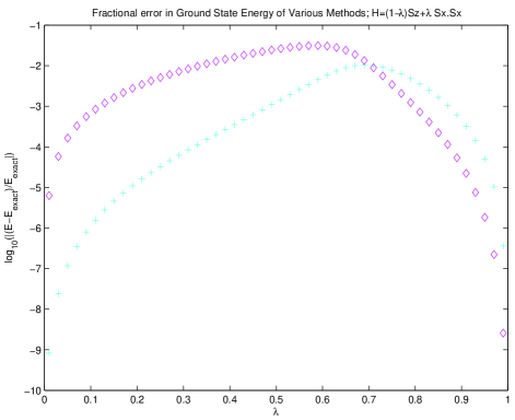
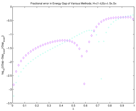
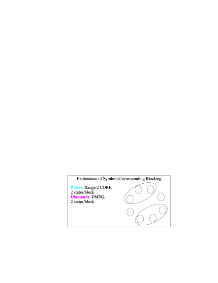
Figure 5: Comparison of CORE to DMRG on an eight-site periodic Ising system. The blocking mimics the intermediate configuration of a DMRG sweep with periodic boundary condition.

IV.2 b. CORE as a disentangling algorithm

The presence of entanglement is often believed to be what makes quantum systems difficult to simulate. By ”entanglement” we mean a measure that quantifies how much a quantum state deviates from a tensor product of states on subsystems. In the case of a pure state, for example, we can measure how much a finite block is entangled to the rest of the system using its von Neumann entropy,

$$S(\rho)=-{\rm Tr}(\rho\ln\rho)$$ (17)

where $\rho$ is the reduced density matrix of the block. Efficient preservation of entanglement accounts for much of DMRG’s successQIDMRG .

Without explicit consideration of entanglement, how does CORE achieve a performance comparable to DMRG? In this subsection we will try to understand this through theoretical comparison with an entanglement-based method.

Vidal recently proposed a method called Entanglement Renormalization (ER) DU , which we can think of as an improvement on HDMRG. Recall that, by HDMRG, we refer to the method that uses reduced density matrix truncation as DMRG does but blocks hierarchically as CORE and naive renormalization do. Vidal observed that before we truncate states in a block according to the reduced density matrix of a target state, it is possible to apply a unitary transformation on the boundary sites of two adjacent blocks and reduce the entanglement of the target state. In other words, the transformation makes states which are truncated away have less weight in the reduced density matrix of the block. Thus the same number of retained states can preserve more of the information of the original system. In exchange, we pay the price that operators acting on one block act on neighboring blocks after the disentangling unitary transformation. The renormalized Hamiltonian can be written as:

$$H^{ER}_{ren}=W^{\dagger}UHU^{\dagger}W,$$

$$U=U_{1,2}\otimes U_{2,3}\otimes...$$ (18)

where the $\{U_{i,i+1}\}$’s are disentangling unitary transformations acting on the edges of neighboring blocks $i,i+1$ and $W$ is an isometric transformation ($W^{\dagger}W=I$) lifting from the coarse-grained subspace to the full Hilbert space. For example, if $\{\left|{a_{i}}\right\rangle\}$ form a basis of the subspace and $\{\left|{b_{i}}\right\rangle\}$ form a basis of the full space, we can write $W_{ij}=\left\langle{b_{i}}|{a_{j}}\right\rangle$, i.e. a matrix whose columns are the basis vectors of the subspace. The orthogonal projection $P$ is related to $W$ by $P=\sum_{k}\left|{a_{k}}\right\rangle\left\langle{a_{k}}\right|=WW^{\dagger}$.

Like CORE, Entanglement Renormalization stores some information in operators in addition to the retained states. The two methods turn out to be have a similar starting point. In Section 2 we have shown the form of the renormalized Hamiltonian in the limit of $t\to\infty$. Now, since both $\{\left|{w_{j}}\right\rangle\}$ and $\{\left|{v_{f(j)}}\right\rangle\}$ (defined in Lemma 1) are orthonormal, we can think of the mapping which identifies each $\{\left|{w_{j}}\right\rangle\}$ with its corresponding $\{\left|{v_{f(j)}}\right\rangle\}$ as the restriction of a unitary transformation which acts on the full Hilbert space. Of course, given our construction we only have the restriction of this transformation to the subspace spanned by the retained states, the extension of the transformation to the full Hilbert space remains undefined and is presumably not unique. The fact that this unitary transformation is not uniquely specified is equivalent to the fact that $W$ and $W^{\dagger}$, which appear in the ER formulas, are isometries and not unitary transformations.

To put the correspondence between CORE and ER in a formal setting we make the following claim:

Claim 2

For all unitary operators $U$ such that $U\left|{v_{f(j)}}\right\rangle=\left|{w_{j}}\right\rangle$,

$$H_{ren}=PUHU^{\dagger}P.$$ (19)

• $$PU = \sum_{i}\left|{w_{i}}\right\rangle\left\langle{w_{i}}\right|U$$

  $$= \sum_{i,l}\left|{w_{i}}\right\rangle\left\langle{w_{i}}\right|U\left|{v_{l}}\right\rangle\left\langle{v_{l}}\right|$$

  $$= \sum_{i,l}\left|{w_{i}}\right\rangle\delta_{f(i)l}\left\langle{v_{l}}\right|$$

  $$= \sum_{i}\left|{w_{i}}\right\rangle\left\langle{v_{f(i)}}\right|$$

  where the third line follows from the observation that $U\left|{v_{l}}\right\rangle$ must be orthogonal to $\cal H^{\prime}$ if $\forall i,~{}l\neq f(i)$. Hence we can write

  $$PUHU^{\dagger}P = \sum_{i,j}\left|{w_{i}}\right\rangle\left\langle{v_{f(i)}}\right|H\left|{v_{f(j)}}\right\rangle\left\langle{w_{j}}\right|$$ (21)

  $$= \sum_{i}\left|{w_{i}}\right\rangle E_{f(i)}\left\langle{w_{i}}\right|$$

  which is exactly Eq.3.  

As we noted earlier, we can write $P=WW^{\dagger}$. In practice, we want to write $H_{ren}$ in a basis of the subspace $\cal H^{\prime}$, so what we really calculate is $H_{ren}=W^{\dagger}UHU^{\dagger}W$, just as in Eq.18. Thus, we see that both CORE and Entanglement Renormalization use a renormalized Hamiltonian of the form $PUHU^{\dagger}P$. The distinction between CORE and ER is that Entanglement Renormalization approximately disentangles a system, while CORE approximates a disentangled system. We say that Entanglement Renormalization approximately disentangles the system because there is no guarantee that we can find disentangling unitaries that reduce the rank of the reduced density matrix to less than or equal to the dimension of retained states. It is usually necessary to truncate some states to keep the degrees of freedom manageable, and information is lost when we truncate the states. CORE approximates a disentangled system in the sense that we first write down the form of a completely disentangled system (Eq.19). Its cluster expansion truncated to diameter-$k$ then approximates this system by ensuring that the new Hamiltonian restricted to any sublattice with diameter less than $k$ is completely disentangled. Here information is lost when we truncate the operators with diameter larger than $k$.

In this picture, the CORE prescription for choosing $R$ and $E_{f(i)}$ is a particular choice of disentangler. One might conceive of a disentangler $PU$ that does not always require overlaps between $\left|{w_{i}}\right\rangle$ and $\left|{v_{f(i)}}\right\rangle$ - a trivial example would be to set $H_{ren}=\sum_{i}\left|{a_{i}}\right\rangle E_{i}\left\langle{a_{i}}\right|$ where $\{\left|{a_{i}}\right\rangle\}$ is the basis of $\cal H^{\prime}$ that we start with. The problem with such an arbitrary choice is that the exact renormalized Hamiltonian could be so non-local that it is difficult to approximate it by a cluster expansion. Our intuition is that by keeping $\left|{w_{i}}\right\rangle$ somewhat ”close” to $\left|{v_{f(i)}}\right\rangle$, cluster expansion can do well. There may be, however, room for improvement once we have a better understanding of the cluster expansion.

IV.3 c. The use of entropy in CORE

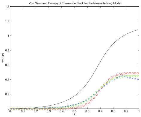
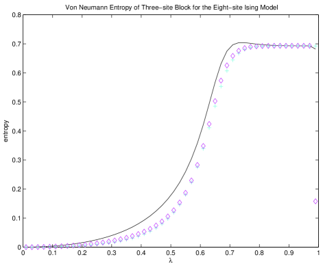
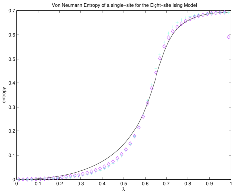
Figure 6: Here we show the block entropy as a function of coupling for the nine-site and eight-site Ising models. The solid curve indicates the exact entropy and other symbols represent methods explained in previous plots. The first two plots are for three-site blocks and the last for a single-site. We see that CORE reproduces the shape in a manner similar to DMRG.

The von Neumann entropy (Eq.17) of finite blocks in a lattice is known to exhibit scaling behaviors with block size that depend on the dimension and phase of the system Latorre . Because DMRG truncates according to the reduced density matrix, entropy can be approximately preserved, so apart from using entropy as a measure of how much information is lost, it is also possible to use the approximate entropy measures from DMRG to detect phase transitions LegezaPT .

Does entropy have a similar use in CORE? Note that CORE is not a variational method that works with a subspace within the original space. It tries to preserve eigenvalues but not the eigenvectors and this allows a disentangling effect. Therefore there is no a priori reason to expect CORE to preserve any particular amount of entropy.

Nonetheless, when we evaluate the three-site block entropy for the two toy models in Section 4(a), we were impressed by how much information CORE captures. Fig.6 shows the entropy of some blocks within the eight-site and nine-site models (the symbols are explained Fig.4 and Fig.5). The first two plots are for a three-site block, in which the eight states are truncated to two after the renormalization. This means that the upper bound of the block entropy changes from $\ln 8$ to $\ln 2$. As it turns out the exact block entropy in the eight-site case is far from saturating the bound, allowing DMRG and CORE to approximate it closely. The third plot in Fig.6 is for the single-site entropy which is available only for the eight-site configuration (The sum of single-site entropies can be used to define the total information encoded in the wavefunctionLegezaEnt ). Here there is no truncation in the site itself, so the entropy upper bound is the same before and after the renormalization.

It may seem confusing how CORE can have a disentangling effect and yet keeps a block entropy that’s comparable to DMRG. By ”disentanglement” we mean a reduction of weight on the eigenvalues of the density matrix outside of the retained space, which does not say anything about the distribution of eigenvalues inside the retained space. It is the latter that determines the block entropy after truncation.

What is remarkable about Fig.6, however, is not the amount of entropy CORE keeps, but the fact that it varies smoothly with the coupling $\lambda$ and has a shape similar to the exact entropy. This raises the possibility that entropy in CORE can also detect quantum phase transitions. Regrettably, unlike Entanglement Renormalization we cannot perform disentangling unitaries without truncation to check entropy scaling in critical and noncritical systemsDU , which means our result can be highly dependent on our choice of retained states and cluster expansion. In absence of more data, we are hesitant to draw conclusions at this point, but this can be an interesting area to explore.

IV.4 d. The choice of retained states

In Fig.4, we have shown two versions of CORE with different choices of retained states, one of which is inspired by DMRG. Although we have not done so, for the study of entropy we just discussed one can even try other variants of DMRG that choose retained states by maximizing entropy QIDMRG or minimizing the Holevo $\chi$ LegezaEnt . How choices of retained states affects the performance of CORE have never been investigated in the past so we would like to briefly discuss it here.

In the single-block calculation it is clear that whatever states we retain, as long as they have an overlap with the lowest lying states of the block, the renormalized range-$1$ (i.e. single site) Hamiltonian will be unchanged. It is only when we compute the connected range-$2$,range-$3$, etc., operators that the difference in choice of retained states show up. In general, the effect of changing the choice of single block retained states can either increase or decrease the size of the longer range connected interactions.

Past works on CORE have exclusively retained states with the smallest energy in the single block Hamiltonian. Let us call this the first version of CORE. Inspired by DMRG, we have tried a second version that uses states with the largest eigenvalues in the reduced density matrix of some target state. When we choose the target state to be the exact ground state of two adjacent blocks, we often obtain a slightly better ground state energy at the expense of a less accurate gap between the ground state and the first excited state, as can be seen in Fig.4. When we choose the target state to be the exact ground state of a larger block that contains our block in the center, however, the retained states often turn out to be the same as those in the first version, i.e., the states with the smallest single block energy. This latter observation is in agreement with the results of Capponi et al Capponi , who found that the retained states in the first version have very high weights in the reduced density matrix of a target state of a larger block.

Capponi et al considered this question in a different context and proposed that one should use the reduced density matrix to check if the truncation in the first version of CORE is justified. We think that such a diagnostic tool has to be used very cautiously. To see why we say this, consider first the case when the target state is calculated on two adjacent blocks. Here the diagnostic tool essentially measures the overlap between $\left|{v_{f(1)}}\right\rangle$ and $\left|{w_{1}}\right\rangle$ (on the Hilbert space of two blocks) in Eq.19. A large overlap, however, does not guarantee that $U$ is close to the identity, let alone a better convergence of the cluster expansion. An alternative is to use the mixed state corresponding to combination of all $\{\left|{v_{f(j)}}\right\rangle\}$ as the target state, which should more meaningfully measures how much $U$ differs from the identity. Yet it still does not in general reliably indicate how well the cluster expansion converges. All we can be certain of is that in the limit $U\to I$, the cluster expansion tends to be exact at nearest neighbor range; this does not tell us much when $U$ is significantly different from $I$. In particular, if we consider the case when the target state is not the ground state on two blocks, but on a larger block containing the block we want to truncate, the situation is even less clear because in that case CORE does not explicitly rotate this ground state to the retained states.

The reduced density matrix tells us a lot in DMRG, but as we have mentioned in the previous subsections, CORE is performing some disentangling action and thus does not preserve the entanglement structure of the states as DMRG does. Simply preserving the most entanglement in the original Hilbert space does not guarantee the most accuracy in CORE. Fortunately, it turns out that in our Ising example, when we choose our retained states to maximize $\left\langle{v_{f(1)}}|{w_{1}}\right\rangle$ on two blocks, we do get a better overall ground state (and sacrifice the accuracies of the excited states). This seems to indicate that the reduced density matrix can be helpful - as long as we remember that even as $\left\langle{v_{f(1)}}|{w_{1}}\right\rangle$ goes to 1, there is no substitute for the longer-range terms in the cluster expansion.

V 6. Discussion and Further Directions

This paper has presented a number of numerical results on various models. While they have shown an usefulness consistent with the considerable body of literature on CORE/RSRG-EI, the picture is still far from clear. The fact that we get an improvement in energy from longe-range operators in 2-D shows non-trivially that there is a genuine small parameter hidden in the cluster expansion, which we believe is associated with the diameter and not the number of blocks in the configuration. Yet we still have little knowledge how this convergence manifests itself under different blocking schemes. When we tested the five-site blocking shown in Section 3(c), we expected the growing spin picture to be valid on prior physical grounds, so we were surprised by how much the long-range terms could affect the result. There seems to be a need for a way to at least estimate the effect of long-range operators. As far as we know, only a very few applications of CORE/RSRG-EI have considered long-range operators up to ”diameter-$\sqrt{2}$” calzado . This is presumably due to limited computational power. Is it possible to use other approximate methods of diagonalization, such as perturbation theory or DMRG, to estimate these long-range operators? This hybrid approach is certainly a direction we would like to pursue in the future.

The second part of the paper, where we compare CORE to entanglement-based approaches, also raises a number of questions. In Section 4(b), we showed that CORE is in fact theoretically similar to Entanglement Renormalization. Naturally, it would be interesting to see how ER performs numerically in comparison to CORE, and in particular, whether one can reproduce the three pictures of the antiferromagnet with ER. Section 4(c) raises the possibility that apart from the energy spectrum, we may be able to use the entropy to study phase transitions with CORE. This, if true, would be remarkable given that CORE was not designed to preserve entropy. In Section 4(d) we mentioned the use of reduced density matrix as an alternative method of deciding what states to keep in each block. There is a special circumstance when it can be important. This has to do with a situation which comes up as soon as one studies frustrated HAF’s where, with increasing frustration, single block levels tend to cross. Since one expects that the most interesting physics of these models is associated with these regions one has to know what states to choose when degeneracies occur. The most obvious solution is to keep all states which can cross as a function of the truncation, however this will increase the complexity of the numerical computations. In that case it may be advantageous to retain the states determined by a DMRG calculation which have the highest weight and correct spin.

Finally, it would be remiss of us not to point out, without giving details, the possibility of adapting the principles of CORE to other applications. We noted in Section 4 that specific truncation and blocking methods are details of the projection operator; the underlying principle is a general one about simplifying states at the expense of generating non-local operators. The principles of DMRG have been generalized to simulate real time evolutionTEBD - Can the principles of CORE can be applied to time evolution as well? There are good motivations for thinking about this. One of the most efficient simulation method for a specific class of unitary evolutions is the stabilizer formalism stabilizer , where we do not keep explicit information about the states and instead keep track of them using a set of operators. Since CORE allows one to calculate expectation values at the expense of state information, we could ask if cluster expansion can be similarly efficient for certain types of unitary evolution. Apart from a direct simulation of unitary evolution, we may also consider turning a unitary evolution problem into a ground state problem using results in quantum complexity theorykitaev (Linear, instead of hierarchical, blocking would have to used in that case). All such possibilities would be interesting to explore.

VI Acknowledgement

We would like to thank Samuel Moukouri for valuable exchanges.

Appendix: QR-Decomposition and Proof of Lemma 1

While constructive proof of Lemma 1 has been given in the pastCOREpaper , for practical implementation, we have found recursive QR-Decomposition to be a fast and convenient way of calculating the rotation $R$ (particularly when packaged libraries such as NAG or LAPACK are available). Given any $M\times N$ matrix $A$, $M\leq N$, the QR-Decomposition is defined by ${\cal QR=A,Q^{T}Q=}I$ where $\cal Q$ is an $M\times M$ matrix and $\cal R$ is an upper-triangular $M\times N$ matrix. For our application, $A$ is simply the overlap matrix $O_{il}$, and the matrix $\cal Q$ plays the role of $R^{\dagger}$ (Thus the $\cal R$ of $\cal QR$ is not the $R$ of Lemma 1). Note that the upper triangular matrix does not necessarily satisfy the contraction condition (Eq.2); it merely guarantees zeros entries below the diagonal $\{{\cal R}(i,i)\mid i=1..M\}$, a particularly weak condition if $M\ll N$. Our solution is to start from the upper-left corner, move down the row and column after every QR-Decomposition until we find another non-zero entry that has non-zero entries below it (this means more than one retained states contract to the eigenstate), at which we perform another QR-Decomposition on the submatrix with that entry as the upper-left corner. We repeat this recursively until the submatrix size is zero.

References

- (1) U. Schollwock, Rev. Mod. Phys. 77, 259 (2005); S. R. White and R. M. Noack, Phys. Rev. Lett. 68, 3487 (1992); Steven R. White, Phys. Rev. B48, 10345 (1993);
- (2) G. Vidal, Phys. Rev. Lett. 91, 147902 (2003); 93, 040502 (2004).
- (3) F. Verstraete, J.I. Cirac, arxiv:cond-mat/0407066
- (4) Y. Shi, L. Duan and G. Vidal, arXiv:quant-ph/0511070
- (5) O. Legeza and J. Solyom, Phys. Rev. Lett. 96, 116401 (2006)
- (6) J.I. Latorre, E. Rico and G. Vidal, Quant. Inf. Comput. 4, 48 (2004); G.Vidal, J.I. Latorre, E. Rico and A. Kitaev, Phys. Rev. Lett. 90, 227902 (2003)
- (7) J. des Cloizeaux, Nuc. Phys. 20, 321-346 (1960); This paper is in response to C. Bloch, Nuc. Phys. 6, 329 (1958)
- (8) T. P. Živković, B. L. Sandleback, T. G. Schmalz, and D. J. Klein, Phys. Rev. B41, 2249 (1990).
- (9) C. J. Morningstar and M. Weinstein, Phys. Rev. Lett. 73, 1873 (1994); C.J. Morningstar and M. Weinstein, Phys. Rev. D54, 4131 (1996).
- (10) K.G. Wilson, Rev. Mod. Phys. 47, 773 (1975)
- (11) J. P. Malrieu and N. Guihery, Phys. Rev. B63 085110 (2001).
- (12) M. Weinstein, Phys. Rev. D61 (2000) 034505; Phys. Rev. B63, 174421
- (13) C.J. Calzado, J.P. Malrieu, Eur. Phys. J B21, 375 (2001); C.J. Calzado, J.P. Malrieu, Phys. Rev. B63, 214520 (2001)
- (14) Some recent papers which feature computations using the CORE technique are: M. Indergand et. al., Phys. Rev. B74, 064429 (2006).; E. Rico, cond-mat/0601254; A. Auerbach, cond-mat/0510738; P. Li and S.Q. Shen, Phys. Rev. B71, 212401 (2005); M.A. Hajj and J.P. Malrieu, Phys. Rev. B72, 094436 (2005); M.A. Hajj et. al., Phys. Rev. B70 094415 (2004);R. Budnik and A. Auerbach, Phys. Rev. Lett. 93, 187205 (2004); S. Capponi et. al.,Phys. Rev. B70, 220505(R) (2004); D. Poilblanc et. al., Phys. Rev. B69, 220406 (2004); D. Poilblanc, D. J. Scalapino and S. Capponi, Phys. Rev. Lett. 91, 137203 (2003); H. Chen et. al., Phys. Rev. B70, 024516 (2004); E. Berg, E. Altman, and A. Auerbach, Phys. Rev. Lett. 90, 147204 (2003); E. Altman and A. Auerbach, Phys. Rev. B65, 104508 (2002); H. Mueller, J. Piekarewicz and J.R. Shepard, Phys. Rev. C66, 024324 (2002);
- (15) In some sense DMRG has analogous issues in terms of optimal lattice site ordering and the choice of a proper basis in two-dimensional systems or models with long-ranged interactions. There entanglement minimization can be used as a criterion: O. Legeza and J. Solyom, Phys. Rev. B68, 195116 (2003); O. Legeza, F. Gebhard and J. Rissler, Phys. Rev. B74, 195112 (2006)
- (16) G. Vidal, arXiv:quant-ph/0512165
- (17) O. Legeza and J. Solyom, Phys. Rev. B70, 205118 (2004)
- (18) S. Capponi, A. Lauchli and M. Mambrini, Phys. Rev. B70, 104424 (2004)
- (19) A.W. Sandvik, Phys. Rev. B56 (1997) 11678
- (20) T.J. Osborne and M.A. Nielsen, arXiv:quant-ph/0109024
- (21) A. Auerbach, Interacting Electrons and Quantum Magnetism, Springer-Verlag, New York, 1994
- (22) D.J.J. Farnell, Phys. Rev. B68, 134419 (2003)
- (23) F. Verstraete, D. Porras and J. I. Cirac, Phys. Rev. Lett. 93, 227205 (2004)
- (24) A. Yu. Kitaev, AH Shen, and MN Vyalyi, Classical and Quantum Computation, American Mathematical Society, Providence, 1999; D. Aharonov, W. Van Dam, J. Kempe, Z. Landau, and S. Lloyd, O. Regev, arXiv:quant-ph/0405098
- (25) D. Gottesman, arXiv:quant-ph/9807006.