Stability of magnetic configurations in nanorings

Abstract

The relative stability of the vortex, onion and ferromagnetic phases in nanorings is examined as a function of the ring geometry. Total energy calculations are carried out analytically, based on simple models for each configuration. Results are summarized by phase diagrams, which might be used as a guide to the production of rings with specific magnetic properties.

I Introduction

The understanding of the properties of small magnetic elements has been a major challenge in the rapidly evolving field of nanoscale science. Besides the basic scientific interest in the magnetic properties of these systems, evidence is that they might be used in the production of magnetic devices, such as high density media for magnetic recording Chou ; zhu and magnetic logic zhu ; logic . Common structures are arrays of nanowires vazquez3 , cylinders cylinders1 ; cylinders2 , cones cones1 ; cones2 and rings rings1 ; rings2 . Recent theoretical studies on such structures have been carried out aiming at determining the stable magnetized state as a function of their geometric details Jubert ; Porrati ; Metlov ; Guslienko . Among the available geometries, the ring shape is of particular interest due to its core-free magnetic configuration leading to uniform switching fields, guaranteeing reproducibility in read-write processes zhu . As a consequence, magnetic nanorings have received increasing attention over the last few years, from both experimental and theoretical points of view.

Geometrically, ring-shaped particles are characterized by their external and internal radii, $R$ and $a$, respectively, and height, $H$. Magnetic measurements as well as micromagnetic simulations of such systems have identified two in-plane magnetic states, namely the flux-closure vortex state, $V$, and the so-called “onion” state, $\mathcal{O}$. The latter is accessible from saturation and is characterized by the presence of two opposite head to head walls klaui1 ; castano1 . In addition, for sufficiently high values of $H$, the occurrence of ferromagnetic order, $F$, along the ring axis, is also possible. It is therefore clear that, for practical applications, the determination of the ranges of values of the parameters $R$, $a$, and $H$, within which one of those configurations is of lowest energy, is of great relevance. However, magnetic measurements do not always allow a clear identification of the magnetic arrangement within the particles, which makes the theoretical approach to the problem highly desirable. In the present work we report results of total energy calculations for magnetic nanorings, on the basis of which the relative stability of the three above mentioned configurations could be determined. Our results are summarized by phase diagrams in the $R-H$ plane.

II Total energy calculations

Nanorings in the size range currently produced may consist of more than $10^{8}$ magnetic atoms. As a consequence, the determination of the configuration of lowest energy based on the investigation of the behavior of individual magnetic moments becomes numerically prohibitive. In order to circumvent this problem, we resort to a simplified description of the system, in which the discrete distribution of magnetic moments is replaced by a continuous one, characterized by the magnetization $\overrightarrow{M}(\vec{r})$, such that $\overrightarrow{M}(\vec{r})\delta V$ gives the total magnetic moment within the element of volume $\delta V$ centered at $\vec{r}$. We also require that $|\vec{M}(\vec{r})|=M_{0}$, the saturation magnetization.

The internal energy, $E_{tot}$, of a single ring is given by the sum of three terms corresponding to the magnetostatic ($E_{dip}$), the exchange ($E_{ex}$), and the anisotropy ($E_{K}$) contributions. Since nanorings are usually polycrystalline, the magnetic anisotropy averages to zero due to the random orientation of the crystallites Klaui . In view of that, it will be neglected in our calculations.

The dipolar contribution can be obtained from the magnetization according to the relation

$$E_{dip}=\frac{\mu_{0}}{2}\int\limits_{V}\overrightarrow{M}(\vec{r})\cdot\nabla U(\vec{r})\;\mbox{d}v\,\,,$$ (1)

where an additional configuration independent term has been left out, and the magnetostatic potential is given (in SI units) by

$$U(\vec{r})=-\frac{1}{4\pi}\int\limits_{V}\frac{\nabla\cdot\overrightarrow{M}(\vec{r}^{\prime})}{\left|\vec{r}-\vec{r}^{\prime}\right|}\mbox{d}v^{\prime}+\frac{1}{4\pi}\int\limits_{S}\frac{\widehat{n}^{\prime}\cdot\overrightarrow{M}(\vec{r}^{\prime})}{\left|\vec{r}-\vec{r}^{\prime}\right|}\mbox{d}s^{\prime}.$$ (2)

In the above expression, $V$ and $S$ represent the volume and surface of the ring, respectively. Assuming that the magnetization varies slowly on the scale of the lattice parameter, the exchange energy can be written as

$$E_{ex}=A\int\limits_{V}\left[\left(\nabla m_{x}\right)^{2}+\left(\nabla m_{y}\right)^{2}+\left(\nabla m_{z}\right)^{2}\right]\mbox{d}v\,\,,$$ (3)

where $m_{i}=M_{i}/M_{0}$ ($i=x,y,z$) are the reduced components of the magnetization and $A$ is the stiffness constant of the material, which depends on the exchange interaction between the magnetic moments. Also in this expression, an additional configuration independent term has been left out aharoni . At this point it is convenient to define dimensionless variables. The natural scale for linear dimensions is given by the exchange length, $L_{ex}=\sqrt{2A/\mu_{0}M_{0}^{2}}$, in terms of which we can define the dimensionless radius and height $\rho=R/L_{ex}$ and $h=H/L_{ex}$, respectively. It is also worth defining the parameter $\gamma=H/R$ and the aspect ratio $\beta=a/R$, such that $0<\beta<1$.

In order to proceed with our calculations, it is necessary to specify the function $\overrightarrow{M}(\vec{r})$ corresponding to each of the three configurations under consideration. For the ferromagnetic state, $\overrightarrow{M}(\vec{r})$ can be approximated by $M_{0}\hat{z}$, where $\hat{z}$ is the unit vector parallel to the axis of the ring, whereas for the vortex state we can take $\overrightarrow{M}(\vec{r})=M_{0}\hat{\phi}$, where $\hat{\phi}$ is the azimuthal unit vector in the ring plane, $xy$. The most interesting case, however, regards the onion configuration, whose typical arrangement of the magnetic moments is illustrated in Fig.(1). So far, no analytical model has been presented in the literature to describe such configuration. However in a recent work, Beleggia et al. beleggia have investigated the magnetic phase diagram for rings, considering a ferromagnetic-in-plane configuration instead of the onion configuration.

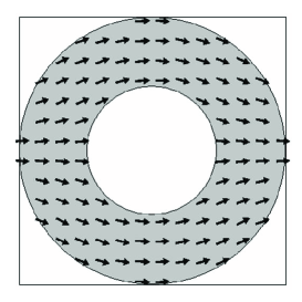
Figure 1: Onion configuration of a Co ring with $h=2.1$, $\rho=7$ and $\beta=0.5$ for $n=4.6$. The arrows denote the direction of the magnetization.

The model we adopt is based on the assumption that the magnetization in the onion configuration can be approximated by

$$\overrightarrow{M}(\vec{r})=M_{r}(\phi)\hat{r}+M_{\phi}(\phi)\hat{\phi}\,\,,$$ (4)

where the possible dependence of $M_{r}$ and of $M_{\phi}$ on $r$ has been neglected. The important point here is the implicit dependence of the two components of the magnetization on the geometry of the ring, more precisely, on the values of $\rho$, $h$ and $\beta$. Therefore, in order to be realistic, any model for the onion configuration has to allow the magnetization either to approach that of an in-plane ferromagnetic or to deviate from it, depending on the values of these parameters. This point will be made clearer further on in this article.

Taking into consideration the spacial symmetry of $\overrightarrow{M}$, as represented in Fig.(1), the expressions for the reduced components $m_{r}=M_{r}/M_{0}$ and $m_{\phi}=M_{\phi}/M_{0}$ of the magnetization can be written as

$$m_{r}(\phi)=\left\{\begin{array}[]{l}f(\phi),\ \ \ \ 0<\phi<\pi/2\\ -f(\pi-\phi),\ \ \ \pi/2<\phi<\pi\\ -f(\phi-\pi),\ \ \ \pi<\phi<3\pi/2\\ f(2\pi-\phi),\ \ \ 3\pi/2<\phi<2\pi\,\,,\end{array}\right.$$ (5)

and

$$m_{\phi}(\phi)=\left\{\begin{array}[]{l}-\sqrt{1-f^{2}(\phi)},\ \ \ \ 0<\phi<\pi/2\\ -\sqrt{1-f^{2}(\pi-\phi)},\ \ \ \pi/2<\phi<\pi\\ \sqrt{1-f^{2}(\phi-\pi)},\ \ \ \pi<\phi<3\pi/2\\ \sqrt{1-f^{2}(2\pi-\phi)},\ \ \ 3\pi/2<\phi<2\pi\,\,,\end{array}\right.$$ (6)

where $f$ is a bounded function such that $-1\leq f(\phi)\leq 1$. A suitable form for the function $f$ is

$$f(n,\phi)=\cos^{n}(\phi)\,\,,$$ (7)

where $n$ is a continuous variable, defined such that $n\geq 1$, chosen so as to minimize the total energy of the configuration for each value of $\rho$, $h$ and $\beta$. Such model allows a continuous transition from the in-plane ferromagnetic state ($n=1$) to the onion state ($n>1$). The deviation from the ferromagnetic configuration becomes more pronounced as $n$ increases from 1. Fig.(1) shows a possible onion configuration with $n>1$.

Having specified the functional form of $\overrightarrow{M}(\vec{r})$ for the three configurations, we are now in position to evaluate the total energy for each of them.

II.1 Ferromagnetic configuration ($F$)

From Eq.(3) we immediately find that $E_{ex}^{F}=0$. Thus, the total energy has only the dipolar contribution, which can be obtained from the magnetostatic potential $U(\vec{r})$ given by Eq.(2). Using the expansion (17) in expression (2) we obtain

$$\tilde{E}_{tot}^{F}\equiv\frac{E_{dip}^{F}}{\mu_{0}M_{0}^{2}L_{ex}^{3}}=\rho^{3}\Psi(\beta,\gamma)\,\,,$$ (8)

where the function $\Psi(\beta,\gamma)$ is defined by

$$\Psi(\beta,\gamma)\equiv\pi\int\limits_{0}^{\infty}\frac{1-e^{-\gamma y}}{y^{2}}\left[J_{1}(y)-\beta J_{1}(\beta y)\right]^{2}\;\mbox{d}y\,\,.$$ (9)

Here $J_{1}(z)$ are Bessel functions of the first kind.

Equation (8) has been previously obtained by Beleggia et al. (See Eq.(15), Ref. beleggia ) considering a more general approach based on Fourier Transforms of the magnetization.

II.2 Vortex configuration ($V$)

It is clear from Eq.(2) that for this configuration $E_{dip}^{V}=0$. The exchange contribution can also be evaluated from Eq.(3) so that the final result for the reduced total energy reads

$$\tilde{E}_{tot}^{V}\equiv\frac{E_{ex}^{V}}{\mu_{0}M_{0}^{2}L_{ex}^{3}}=-\pi h\ln\beta\,\,.$$ (10)

II.3 Onion configuration ($\mathcal{O}$)

In the previous two configurations, the magnetization function satisfies the condition $\nabla\cdot\overrightarrow{M}=0$, which means absence of volumetric magnetic charges. In the onion configuration, however, due to the presence of two regions with head-to-head domain walls, in which $\nabla\cdot\overrightarrow{M}\neq 0$, the dipolar energy turns out to be given by the sum of two contributions, $E_{dS}^{\mathcal{O}}$ and $E_{dV}^{\mathcal{O}}$, coming from the surface and volume terms in the expression for $U(\vec{r})$, respectively. Details of the calculations of these two quantities are given in the Appendix. Results for the reduced energies read

$$\tilde{E}_{dS}^{\mathcal{O}}\equiv\frac{E_{dS}^{\mathcal{O}}}{\mu_{0}M_{0}^{2}L_{ex}^{3}}=\rho^{3}\sum_{p=1}^{\infty}b_{p}\left(b_{p}Q_{1}+d_{p}Q_{2}\right)\,,$$ (11)

$$\tilde{E}_{dV}^{\mathcal{O}}\equiv\frac{E_{dV}^{\mathcal{O}}}{\mu_{0}M_{0}^{2}L_{ex}^{3}}=\rho^{3}\sum_{p=1}^{\infty}(d_{p}-b_{p})\left(b_{p}Q_{3}+d_{p}Q_{4}\right)\,,$$ (12)

where

$$b_{p}(n) = \int\limits_{0}^{\pi/2}f(n,\phi)\cos(p\phi)\;\mbox{d}\phi\,\,,$$ (13)

$$d_{p}(n) = p\int\limits_{0}^{\pi/2}\sqrt{1-f^{2}(n,\phi)}\sin(p\phi)\;\mbox{d}\phi\,\,,$$ (14)

and

$$Q_{1}(\beta,\gamma)=\frac{4}{\pi}\int\limits_{\beta}^{1}x\;\mbox{d}x\int\limits_{0}^{\infty}\mbox{d}y\left[J_{p}(y)-\beta J_{p}(\beta y)\right]\\ \left(\frac{e^{-\gamma y}+\gamma y-1}{y}\right)\left[J_{p-1}(xy)-J_{p+1}(xy)\right]\,\,,$$

$$Q_{2}(\beta,\gamma)=\frac{8}{\pi}\int\limits_{\beta}^{1}\mbox{d}x\int\limits_{0}^{\infty}\mbox{d}y\left[J_{p}(y)-\beta J_{p}(\beta y)\right]\\ \left(\frac{e^{-\gamma y}+\gamma y-1}{y^{2}}\right)J_{p}(xy)\,\,,$$

$$Q_{3}(\beta,\gamma)=\frac{4}{\pi}\int\limits_{\beta}^{1}\mbox{d}w\int\limits_{\beta}^{1}x\;\mbox{d}x\int\limits_{0}^{\infty}\mbox{d}y\left[J_{p-1}(xy)-J_{p+1}(xy)\right]\\ \left(\frac{e^{-\gamma y}+\gamma y-1}{y}\right)J_{p}(wy)\,,$$

$$Q_{4}(\beta,\gamma)=\frac{8}{\pi}\int\limits_{\beta}^{1}\mbox{d}w\int\limits_{\beta}^{1}\mbox{d}x\int\limits_{0}^{\infty}\mbox{d}y\;J_{p}(wy)\\ \left(\frac{e^{-\gamma y}+\gamma y-1}{y^{2}}\right)J_{p}(xy)\,\,.$$

We remark that the sum in Eqs. (11) and (12) runs over odd values of $p$ and converges quite rapidly so that, in practice, just a few values of $p$ (say, 5 or 6) have to be considered.

The exchange energy can be also obtained analytically, as indicated in the Appendix. The reduced energy $\tilde{E}_{ex}^{\mathcal{O}}$ is then given by

$$\tilde{E}_{ex}^{\mathcal{O}}\equiv\frac{E_{ex}^{\mathcal{O}}}{\mu_{0}M_{0}^{2}L_{ex}^{3}}=-\pi h\left[I(n)-1\right]\ln\beta\,,$$ (15)

where

$$I(n)=\frac{2}{\pi}\int\limits_{0}^{\pi/2}\frac{1}{1-f^{2}(n,\phi)}\left[\frac{\partial f(n,\phi)}{\partial\phi}\right]^{2}\;\mbox{d}\phi\,.$$

As already pointed out, the value of $n$ in the above expressions is chosen so as to minimize the total energy, for fixed values of the geometrical parameters $\beta$, $\gamma$ and $\rho$. In other words, it is obtained by solving the equation $\partial\tilde{E}_{tot}^{\mathcal{O}}/\partial n=0$, where $\tilde{E}_{tot}^{\mathcal{O}}=\tilde{E}_{dS}^{\mathcal{O}}+\tilde{E}_{dV}^{\mathcal{O}}+\tilde{E}_{ex}^{\mathcal{O}}$. It is worth pointing out that the dependence of $\tilde{E}_{tot}^{\mathcal{O}}$ on $n$ enters just via the functions $b_{p}(n)$, $d_{p}(n)$ and $I(n)$. The first one can be expressed in terms of Gamma functions, whereas the remaining two can be easily evaluated numerically. On the other hand, the functions $Q_{j}$ can be calculated just once for given values of $\beta$ and $\gamma.$

III Results and Discussion

The above expressions for the total energy enable us to investigate the relative stability of the three configurations of interest. For each aspect ratio $\beta$ we can determine the ranges of values of the dimensionless radius $\rho$ and height $h$ within which one of the three configurations is of lowest energy. The boundary line between any two configurations can be obtained by equating the expressions for the corresponding total energies. Figure (2) illustrates phase diagrams for different values of $\beta$. The stability regions corresponding to each configuration are indicated in the diagram.

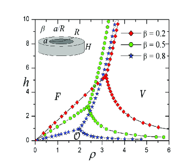
Figure 2: Magnetic phase diagrams for rings with $\beta=a/R=0.2$ (diamonds), $0.5$ (full circles), and $0.8$ (stars). $F$, $V$ and $\mathcal{O}$ indicate regions where ferromagnetic out-of-plane, vortex and onion configurations are relatively more stable. $h$ and $\rho$ are the dimensionless geometric parameters, defined respect to the material exchange length as $h=H/L_{ex}$ and $\rho=R/L_{ex}$. The inset illustrates the geometry of a ring.

It is interesting to look at the dependence of the exponent $n$, which determines the magnetization profile in the lower energy onion configuration, on the geometry of the ring. Fig.(3) presents a set of lines in the $\rho h$-plane corresponding to constant values of $n$, for $\beta=0.5$. The points on such lines laying outside the $\mathcal{O}$ region (open symbols) correspond to either metastable or unstable onion configurations. We shall come back to this point further on in this article. We clearly see that for small rings, the onion configuration turns out to be rather close to the in-plane ferromagnetic one ($n=1$). Another interesting point is the weak dependence of the in-plane magnetization of the onion configuration as a function of $n$. The reduced magnetization $\overline{m}_{x}$ can be obtained by integrating $M_{x}$ within the volume of the ring, which gives us $\overline{m}_{x}=\left(2/\pi\right)\left[{b}_{{1}}{(n)+d}_{{1}}{(n)}\right]$. The inset in Fig.(3) presents $\overline{m}_{x}$ as a function of $n$, which well illustrates this point.

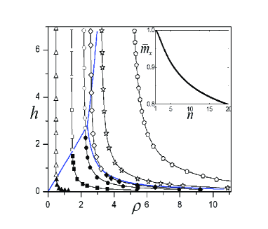
Figure 3: Constant $n$ curves for rings with $\beta=0.5$. Solid symbols correspond to stable onion configurations, and open symbols to metastable or unstable ones. Thick solid lines denote the boundaries between stability regions and thin lines are guides to the eye. Results are presented for $n=1.01$ (triangles), $n=1.1$ (squares), $1.3$ (circles), 1.5 (diamonds), 2 (stars), and 4 (pentagons). Inset: magnetization component along the onion axis ($m_{x}$) as a function of constant-$n$ curves in the $\rho h$-plane for rings with $\beta=0.5$. Results are presented for rings both inside (full symbols) and outside (open symbols) the onion stability region. The latter correspond to either unstable or metastable onion configurations.

The transition between the $F$ and $\mathcal{O}$ configurations is determined by the balance between the energies of the out-of-plane and of the in-plane magnetic configurations. A qualitative understanding of such transition can be achieved by examining the strength of the demagnetization fields along the $z$ and $x$ axes. For given $\beta$ and $\rho$, larger values of $h$ result in reduced demagnetization fields along the $z$ direction, favoring the $F$ configuration. This is the case, for example, of rings with $\rho=1.0$ and $\beta=0.2$, when $h$ is increased from 1.0 to 3.0. On the other hand, for fixed $\rho$ and $h$, a decrease in $\beta$ is equivalent to a reduction of the inner radius, which results in a larger in plane demagnetizing field. Thus, a ring with $\rho=1.0$ and $h=1.0$ exhibits an in-plane magnetic order for $\beta=0.2$, and an out-of-plane order for $\beta=0.8$.

Concerning the two in-plane configurations, namely $\mathcal{O}$ and $V$, the transition between them depends on the strength of the demagnetization field along the $x$ direction in the domain wall regions of the $\mathcal{O}$ configuration. The larger the value of the ring width $W=R-a$, the smaller this field is, favoring the onion state. Thus, a ring with $\rho=3.0$ and $h=1.0$ exhibits the $V$ phase for $\beta=0.8$, and the $\mathcal{O}$ configuration for $\beta=0.2$.

The mechanism responsible for the transition between the $V$ and $F$ configurations is somewhat subtle. We notice in Fig.(2) that the line separating these two regions exhibits a maximum shift to the left for $\beta$ about 0.5. As a consequence, rings with say $\rho=3.0$, $h=6.0$ and inner radius corresponding to $\beta=$ 0.2, 0.5, and 0.8 are found to exhibit $F$, $V$, and $F$ configurations, respectively. Such interesting behavior can be understood by considering the relative strength of the exchange and dipolar energies in the two states. It is clear from Eq.(10) that for fixed values of  $\rho$ and $h$ the exchange energy in the vortex state diverges at $\beta=0$, whereas that for the $F$ configuration approaches a finite value [cf. Eqs(8) and (9)]. Thus, for sufficiently small inner radii ($\beta\ll 1$), the $F$ configuration has lower energy than the $V$ one. The reason for that is the large contribution to $E_{ex}^{V}$ coming from the central region of the ring. Then, the increase in the inner radius leads to a rapid decrease of $E_{ex}^{V}$, reducing $E_{tot}^{V}$ with respect to $E_{tot}^{F}$ and favoring the $V$ configuration for intermediate values of $\beta$. However, for values of $\beta$ close to 1 (narrow rings) and sufficiently large values of $h$, the dipolar energy in the $F$ state, which can be associated to the magnetic charges at the top and bottom surfaces of the ring, becomes smaller than $E_{ex}^{V}$, favoring the ferromagnetic state.

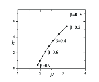
Figure 4: Triple point position ($\rho_{t},h_{t}$) as a function of $\beta=a/R$ (full circles). The result for a cylinder is represented by a star.

All diagrams in Fig.(2) show a triple point ($\rho_{t},h_{t}$), corresponding to the situation in which the three configurations have equal energy. Fig.(4) shows the trajectory of the triple point ($r_{t}(\beta),h_{t}(\beta)$) as a function of $\beta$. We notice that the curve correctly extrapolates to the result for cylinders, which has been numerically obtained by d’Albuquerque e Castro et al. scaling1 using a scaling technique, and analytically, by Landeros et al. landerosscaling .

An interesting result is the occurrence in some cases of metastable onion configurations. Castaño et al. castano1 have carried out a detailed experimental study of the magnetic behavior of Co nanorings with $H=10$ nm and external and inner radii ranging from $90$ nm to $260$ nm and from $20$ nm to $140$ nm, respectively. For rings with $R=180$ nm and $a=20$ nm, and $R=180$ nm and $a=70$ nm, they have found that the corresponding hysteresis curves clearly indicate the occurrence of metastable onion configurations. Such states can be reached by reducing the applied magnetic field from the saturation value to zero. However, as the magnetic field is increased in the opposite direction and the magnetic energy becomes sufficiently high to overcome the energy barrier between the $\mathcal{O}$ and $V$ configurations, the systems undergoes a transition to the latter state. Such behavior is entirely consistent with our results. Indeed, taking into consideration that for Co $L_{ex}=2.85$ nm, the rings examined by Castaño and collaborators have reduced dimensions $\rho=63.2$, and $h=3.5$ and correspond to $\beta=0.11$ and 0.39. Thus, from the results in Fig. (2), we expect the two rings to fall well within the vortex region. We remark that from Fig. (4), the upper bound for the position of the triple point for $\beta\rightarrow 0$, is $\rho_{max}=3.8$ which is much smaller than the value corresponding to the two samples. As a consequence, the observed onion configurations in such systems represent necessarily metastable states. The occurrence of metastable onion states within the vortex region has also been found in micromagnetic calculations. Using the OOMMF package OOMMF we have carried out ground state calculations for a Co ring with $h=2.1$, $\rho=7$, and $\beta=0.5$. We have found that the system might be trapped in a metastable onion configuration when the in-plane ferromagnetic state is taken as the starting configuration. These results are presented in Fig.(1).

In conclusion, we have theoretically investigated the dependence of the internal magnetic configuration of nanorings on their geometry. Three typical configurations have been considered, namely out-of-plane ferromagnetic, vortex, and the so-called onion configuration. For the latter, we have proposed a simple analytical model, which allows a continuum transition between the onion and the in-plane ferromagnetic states. Our results are summarized in phase diagrams giving the relative stability of the three configurations. The possibility of the systems assuming unstable or metastable configurations has also been considered. Our results might be used as a guide to experimentalists interested in producing samples with specific magnetic properties.

IV Appendix

The calculation of the dipolar energy of the onion configuration begins by replacing the functional form Eq. (4) in Eq. (1), leading to

$$E_{dip}^{\mathcal{O}}=\frac{\mu_{0}}{2}\int\limits_{V}\left[M_{r}\left(\phi\right)\frac{\partial U}{\partial r}+\frac{M_{\phi}\left(\phi\right)}{r}\frac{\partial U}{\partial\phi}\right]\mbox{d}v\,.$$ (16)

For the calculation of the magnetostatic potential we use expression (4) and the following expansion Jackson

$$\frac{1}{\left|\vec{r}-\vec{r}^{\prime}\right|}=\sum_{p=-\infty}^{\infty}e^{ip(\phi-\phi^{\prime})}\int\limits_{0}^{\infty}J_{p}(kr)J_{p}(kr^{\prime})e^{k(z_{<}-z_{>})}\mbox{d}k,$$ (17)

where $J_{p}$ are the first kind Bessel functions. This way the surface contribution to the potential (second term in Eq.(2)), reads

$$U_{S}=\frac{M_{0}}{4\pi}\sum_{p=-\infty}^{\infty}e^{ip\phi}\int\limits_{0}^{2\pi}m_{r}\left(\phi^{\prime}\right)e^{-ip\phi^{\prime}}\mbox{d}\phi^{\prime}\\ \int\limits_{0}^{\infty}\mbox{d}k\;J_{p}(kr)\left[RJ_{p}\left(kR\right)-aJ_{p}(ka)\right]\int\limits_{0}^{H}e^{k\left(z_{<}-z_{>}\right)}\;\mbox{d}z^{\prime}\,.$$

Using $m_{r}\left(\phi\right)$ defined by Eq. (5) it is straightforward to obtain

$$\int\limits_{0}^{2\pi}m_{r}\left(\phi\right)e^{-ip\phi}\;\mbox{d}\phi=2\left(1-e^{-ip\pi}\right)b_{p}\,,$$

where $b_{p}$ is defined by Eq. (13). This relation lead us to consider only odd values of the sum index $p$ in what follows. Integrating over $z^{\prime}$, and after some manipulations, we obtain that

$$U_{S} = \frac{2M_{0}}{\pi}\sum_{p=1}^{\infty}b_{p}\cos(p\phi)\!\!\int\limits_{0}^{\infty}\mbox{d}k\;J_{p}(kr)$$

$$\times\left[RJ_{p}\left(kR\right)-aJ_{p}(ka)\right]\left[\frac{2-e^{-kz}-e^{-k(H-z)}}{k}\right]\,.$$

Introducing this potential in Eq. (16) we obtain

$$E_{dS}^{\mathcal{O}}=\frac{\mu_{0}M_{0}^{2}}{\pi}\sum_{p=1}^{\infty}b_{p}\int\limits_{0}^{\infty}\frac{\mbox{d}k}{k}\int\limits_{0}^{H}\mbox{d}z\left[2-e^{-kz}-e^{-k(H-z)}\right]$$ (18)

$$\times \!\!\!\!\!\!\left.\int\limits_{a}^{R}\mbox{d}r\left[RJ_{p}(kR)-aJ_{p}(ka)\right]\right\{\frac{kr}{2}\left[J_{p-1}(kr)-J_{p+1}(kr)\right]$$

$$\times \!\!\left.\!\!\!\!\int\limits_{0}^{2\pi}\mbox{d}\phi\;\left[m_{r}(\phi)\cos(p\phi)-J_{p}(kr)p\,m_{\phi}(\phi)\sin(p\phi)\right]\right\}\,.$$

Using

$$\int\limits_{0}^{2\pi}m_{r}\left(\phi\right)\cos(p\phi)\;\mbox{d}\phi=4b_{p}$$

and

$$p\int\limits_{0}^{2\pi}m_{\phi}\left(\phi\right)\sin(p\phi)\;\mbox{d}\phi=-4d_{p}\,,$$

in Eq. (18) we obtain

$$E_{dS}^{\mathcal{O}} = \mu_{0}M_{0}^{2}R^{3}\sum_{p=1}^{\infty}\frac{8}{\pi}\int\limits_{0}^{\infty}\mbox{d}y$$

$$\left[J_{p}\left(y\right)-\beta J_{p}(\beta y)\right]\left(\frac{e^{-\gamma y}+\gamma y-1}{y^{2}}\right)$$

$$\int\limits_{\beta}^{1}\mbox{d}x\left\{b_{p}d_{p}J_{p}(xy)+b_{p}^{2}\frac{xy}{2}\left[J_{p-1}(xy)-J_{p+1}(xy)\right]\right\}\,.$$

Thus, the superficial contribution to the reduced dipolar energy (Eq. (11)) can be written as

$$\tilde{E}_{dS}^{\mathcal{O}}\equiv\frac{E_{dS}^{\mathcal{O}}}{\mu_{0}M_{0}^{2}L_{ex}^{3}}=\rho^{3}\sum_{p=1}^{\infty}b_{p}\left(b_{p}Q_{1}+d_{p}Q_{2}\right)\,.$$

The calculation of the volumetric contribution (Eq. (12)) follow the same procedure.

The exchange energy of the onion configuration comes from substituting the Cartesian magnetization components

$$m_{x}\left(\phi\right) = m_{r}\left(\phi\right)\cos(\phi)-m_{\phi}\left(\phi\right)\sin(\phi)$$

$$m_{y}\left(\phi\right) = m_{r}\left(\phi\right)\sin(\phi)+m_{\phi}\left(\phi\right)\cos(\phi)\,,$$

in the semiclassical expression Eq. (3), from which we obtain that

$$\tilde{E}_{ex}^{\mathcal{O}}=\frac{h}{2}\log\frac{1}{\beta}\int\limits_{0}^{2\pi}\left[\left(\frac{\partial m_{r}}{\partial\phi}-m_{\phi}\right)^{2}+\left(\frac{\partial m_{\phi}}{\partial\phi}+m_{r}\right)^{2}\right]\mbox{d}\phi\,.$$

By using Eqs. (5) and (6) we found the reduced exchange energy of the onion configuration (Eq. 15).

References

- (1) S. Y. Chou, Proc. IEEE 85, 652 (1997); G. Prinz, Science 282, 1660 (1998).
- (2) J-G. Zhu, Y. Zheng, and Gary A. Prinz, J. Appl. Phys. 87, 6668 (2000).
- (3) R. P. Cowburn and M. E. Welland, Science 287, 1466 (2000)
- (4) M. Vázquez, Physica B 299, 302–313 (2001)
- (5) R. P. Cowburn, D. K. Koltsov, A. O. Adeyeye, M. E. Welland, and D. M. Tricker, Phys. Rev. Lett. 83, 1042 (1999).
- (6) C. A. Ross, M. Hwang, M. Shima, J. Y. Cheng, M. Farhoud, T. A. Savas, Henry I. Smith, W. Schwarzacher, F. M. Ross, M. Redjdal, and F. B. Humphrey, Phys. Rev. B 65, 144417 (2002)
- (7) J. N. Chapman, P. R. Aitchisom, K. J. Kirk, S. McVitie, J. C. S. Kools, and M. F. Gillies, J. Appl. Phys. 83, 5321 (1998).
- (8) C. A. Ross and M. Farhoud and M. Hwang and H. I. Smith and M. Redjdal and F. B. Humphrey, J. Appl. Phys. 89, 1310 (2001).
- (9) F. J. Castaño, C. A. Ross, A. Eilez, W. Jung, and C. Frandsen, Phys. Rev. B 69, 144421 (2004)
- (10) J. Rothman, M. Kläui, L. Lopez-Diaz, C. A. F. Vaz, A. Bleloch, J. A. C. Bland, Z. Cui, and R. Speaks, Phys. Rev. Lett. 86, 1098 (2001).
- (11) P. O. Jubert, and R. Allenspach, Phys. Rev. B 70, 144402 (2004).
- (12) F. Porrati, and M. Huth, Appl. Phys. Lett. 85, 3157 (2004).
- (13) Konstantin L. Metlov, and Konstantin Yu. Guslienko, J. Magn. Magn. Mater. 242-245, 1015 (2002).
- (14) K. Yu. Guslienko and V. Novosad, J. Appl. Phys. 96, 4451 (2004).
- (15) M. Kläui, C. A. F. Vaz, J. A. C. Bland, T. L. Monchesky, J. Unguris, E. Bauer, S. Cherifi, S. Heun, A. Locatelli, L. J. Heyderman and Z. Cui, Phys. Rev. B 68, 134426 (2003)
- (16) F. J. Castaño, C. A. Ross, C. Frandsen, A. Eilez, D. Gil, Henry I. Smith, M. Redjdal and F. B. Humphrey, Phys. Rev. B 67, 184425 (2003).
- (17) M. Klaui, C. A. F. Vaz, L. Lopez-Diaz and J.A. C. Bland, J. Phys.: Condens. Matter. 15, R985 (2003).
- (18) A. Aharoni, Introduction to the Theory of Ferromagnetism (Clarendon Press, Oxford, 1996).
- (19) M. Beleggia, J. W. Lau, M. A. Schofield, Y. Zhu, S. Tandon and M. De Graef, J. Magn. Magn. Mat. 301, 131 (2006).
- (20) J. d’Albuquerque e Castro, D. Altbir, J. C. Retamal and P. Vargas, Phys. Rev. Lett. 88, 237202 (2002).
- (21) P. Landeros, J. Escrig, D. Altbir, J. d’Albuquerque e Castro and P. Vargas, Phys. Rev. B 71, 94435 (2005).
- (22) The public domain package is available at math.nist.gov/oommf.
- (23) J. D. Jackson, Classical Electrodynamics, 2nd Edition (John Wiley & Sons, 1975).