Magnon Decay in Noncollinear Quantum Antiferromagnets

Abstract

Instability of the excitation spectrum of an ordered noncollinear Heisenberg antiferromagnet (AF) with respect to spontaneous two-magnon decays is investigated. We use a spin-1/2 AF on a triangular lattice as an example and examine the characteristic long- and short wave-length features of its zero-temperature spectrum within the $1/S$-approximation. The kinematic conditions are shown to be crucial for the existence of decays and for overall properties of the spectrum. The $XXZ$ and the $J$–$J^{\prime}$ generalizations of the model, as well as the role of higher-order corrections are discussed.

A quantum many-body system with nonconserved number of particles may have cubic vertices, which describe interaction between one- and two-particle states. In crystals such anharmonicities lead to finite thermal conductivity by phonons ziman . In the superfluid ⁴He, the cubic interaction between quasiparticles result in a complete wipeout of the single-particle branch at energies larger than twice the roton energy pitaevskii .

In quantum magnets with collinear spin configuration, e.g., in AF on a bipartite lattice, cubic terms are absent and anharmonicities are of higher order collinear . The cubic terms can appear due to dipolar interactions akhiezer , but in magnetic insulators those are weak and usually can be neglected. It has been gradually realized that substantial cubic interactions should exist in the noncollinear AFs miyake ; ohyama ; chubukov94 ; Zh_nikuni . Qualitatively, such cubic anharmonic terms arise due to coupling of the transverse (one-magnon) and the longitudinal (two-magnon) fluctuations in these systems.

The noncollinearity of an antiferromagnetic spin configuration can be either induced by external magnetic field Zh_nikuni or by frustrating effect of the lattice (e.g., in the triangular lattice (TL) spins form the so-called 120^∘ structure miyake ; chubukov94 ). In the former case, spontaneous decays are allowed above a threshold field $H^{*}$, such that magnons become strongly damped throughout the Brillouin zone (BZ) field . On the other hand, the role of magnon interactions in the spectra of frustrated AFs is not well understood. The earlier work on TLAF chubukov94 has discussed only renormalization of the spin-wave velocities. The recent series expansion study Singh has found a substantial deviation of the spectrum from the linear spin-wave theory (LSWT) and interpreted it as a sign of spinons. The latest work Starykh has questioned this hypothesis by showing that $1/S$ expansion strongly modifies the LSWT spectrum leading to an overall agreement with the numerical data. However, the subject of spontaneous decays has been hardly touched upon. Astonishingly, instability of the single-particle spectrum in the presence of a well-defined, magnetically ordered ground state is, perhaps, the single most striking qualitative difference of the non-collinear AFs from the collinear ones.

In this Letter, we shall study magnon decay in noncollinear quantum AFs at $T=0$ using an example of the Heisenberg AF on a TL. The noncollinearity is necessary but not sufficient for decays. In addition, the energy and momentum must be conserved within a decay process (kinematic conditions). Thus, the decays are determined, in part, by the shape of the single-particle dispersion that may, or may not, allow spontaneous decays. We analyze singularities in the two-magnon continuum that outline instability regions or lead to discontinuities in the single-particle spectrum. Our long wave-length analysis yields definite asymptotic statements regarding the life-time of magnetic excitations. We discuss briefly the $XXZ$ and $J$–$J^{\prime}$ models where noncollinearity is also present.

We begin by rewriting the spin-$S$, nearest-neighbor Heisenberg Hamiltonian for the TLAF into the local rotating frame associated with the classical 120^∘ structure of the spins, and proceed with the standard Holstein-Primakoff transformation of the spin operators into bosons followed by the Bogolyubov transformation diagonalizing the harmonic part of the bosonic Hamiltonian. This procedure leads to the following Hamiltonian:

$$\hat{\cal H}=\sum_{\bf k}\varepsilon_{\bf k}b^{\dagger}_{\bf k}b_{\bf k}+\frac{1}{2}\sum_{{\bf k},{\bf q}}V_{{\bf k},{\bf q}}\left(b^{\dagger}_{\bf k-q}b^{\dagger}_{\bf q}b_{\bf k}+{\rm h.c.}\right)+...\,,$$ (1)

where the ellipses stand for the classical energy, other 3-boson terms that do not lead to decays, 4-boson, and the higher-order terms. Although we will need some of these other terms for the $1/S$-expansion below, Eq. (1) will suffice for the purpose of this paper. All of the necessary terms can be found in miyake ; chubukov94 . The LSWT magnon energy and the 3-boson vertex in Eq. (1) are given by:

$$\varepsilon_{\bf k}=3JS\sqrt{(1-\gamma_{\bf k})(1+2\gamma_{\bf k})}\ ,$$ (2)

$$V_{{\bf k},{\bf q}}=3iJ\sqrt{3S/2}\>\big{[}f_{{\bf q},{\bf q^{\prime}},{\bf k}}+f_{{\bf q^{\prime}},{\bf q},{\bf k}}-g_{{\bf k},{\bf q},{\bf q^{\prime}}}\big{]}$$ (3)

where $J$ is the exchange constant, ${\bf q^{\prime}}\!=\!{\bf k}\!-\!{\bf q}$, $f_{1,2,3}=\bar{\gamma}_{1}(u_{1}+v_{1})(u_{2}u_{3}+v_{2}v_{3})$, $g_{1,2,3}=\bar{\gamma}_{1}(u_{1}+v_{1})(u_{2}v_{3}+v_{2}u_{3})$, $\gamma_{\bf k}=\frac{1}{3}(\cos k_{x}+2\cos\frac{k_{x}}{2}\cos\frac{\sqrt{3}k_{y}}{2})$, $\bar{\gamma}_{\bf k}=\frac{1}{3}(\sin k_{x}-2\sin\frac{k_{x}}{2}\cos\frac{\sqrt{3}k_{y}}{2})$, and $u$, $v$ are the Bogolyubov coefficients: $2u_{i}^{2}-1=3JS(1+\frac{1}{2}\gamma_{i})/\varepsilon_{i}$, $u_{i}^{2}-v_{i}^{2}=1$.

Kinematics: long wave-length limit. — The magnon branch in Eq. (2) has three zero-energy modes: ${\bf k}=0$ and ${\bf k}\!=\!\pm\!{\bf Q}\!=\!(\pm\frac{4}{3}\pi,0)$, points $\Gamma$, and K (K’) in Fig. 1, respectively. In contrast with a square-lattice AF, velocities of these Goldstone modes are different: $c_{0}\!=\!\sqrt{3/4}$ and $c_{\pm Q}\!=\!\sqrt{3/8}$ (in units of $3JSa$). This immediately implies that excitations with ${\bf k}\rightarrow 0$ are kinematically unstable towards decays into $({\bf q},{\bf q}^{\prime})\rightarrow({\bf Q},-{\bf Q})$ ones, in close analogy with a decay of a longitudinal phonon into two transverse ones ziman . Clearly, such decays are immune to $1/S$ corrections as long as velocities remain different. This picture is pertinent to all other non-collinear AF with more than one Goldstone mode.

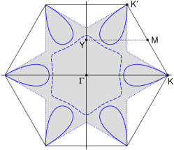
Figure 1: (color online). Brillouin zone of the TL. The shaded area corresponds to the region where spontaneous two-magnon decays are allowed. $\Gamma=(0,0)$, K=$(4\pi/3,0)$, K’=$(2\pi/3,2\pi/\sqrt{3})$, Y=$(0,\pi/\sqrt{3})$, and M=$(\pi,\pi/\sqrt{3})$ points are highlighted. The lines correspond to the extrema in the two-magnon continuum described in the text.

For magnons at small $\tilde{\bf k}={\bf k}-{\bf Q}$ there exists a more subtle reason for decays. Instead of the usual convex and isotropic form, the magnon energy is nonanalytic with varying convexity: $\varepsilon_{\bf k}\approx c_{Q}\tilde{k}(1-\alpha_{\varphi}\tilde{k})$, where $\alpha_{\varphi}\sim\cos 3\varphi$. This form together with the commensurability of the ordering vector create kinematic conditions for the decays from the steeper side of the energy cone at ${\bf k}\rightarrow{\bf Q}$ into the less steeper sides at ${\bf q},{\bf q}^{\prime}\rightarrow-{\bf Q}$. Thus, magnons near the ${\bf Q}$-point are unstable only in a range of angles. Although such conditions are more delicate, it is very unlikely that the higher-order terms would selectively cancel the nonanalyticity. Therefore, the ${\bf k}\rightarrow{\bf Q}$ decays should be prominent in the TLAF.

Kinematics: full BZ. — In the model (1) an excitation with the momentum ${\bf k}$ is unstable if the minimum energy of the two-particle continuum, $E_{{\bf k},{\bf q}}=\varepsilon_{\bf q}+\varepsilon_{{\bf k}-{\bf q}}$, is lower than $\varepsilon_{\bf k}$. Then the boundary between stable and unstable excitations is where such a minimum crosses the single-particle branch and the decay condition $E_{{\bf k},{\bf q}}=\varepsilon_{\bf k}$ is first met. Thus, to find these boundaries one should analyze the extrema of the continuum. For a gapless spectrum there can be several solutions as we show for the TLAF:
(a) Decay with emission of a ${\bf q}=0$ magnon. $E_{{\bf k},0}\equiv\varepsilon_{\bf k}$ for any ${\bf k}$ but it never crosses the magnon branch.
(b) Decay with emission of ${\bf q}=\pm{\bf Q}$ magnons. Equation that defines the boundary is $E_{{\bf k},{\bf Q}}\equiv\varepsilon_{{\bf k}\pm{\bf Q}}=\varepsilon_{\bf k}$ and its solution is shown by the dotted line in Fig. 1. The shaded area is where magnon decays are allowed. It can be shown that $E_{{\bf k},{\bf Q}}$ corresponds to an absolute minimum of the continuum within the shaded area. In accord with our long wave-length discussion, the area around ${\bf k}=0$ is enclosed and it is a finite segment in the vicinity of the ${\bf Q}$-point where decays are allowed.
(c) Decay into two identical magnons. The two-magnon continuum has extrema that are found from $\partial E_{{\bf k},{\bf q}}/\partial{\bf q}=0$ pitaevskii ; field . This condition means that the products of decay have equal velocities. The simplest way to satisfy that is to assume that their momenta are also equal. This is fulfilled automatically if ${\bf q}=({\bf k}+{\bf G}_{i})/2$, where ${\bf G}_{i}$ is one of the two reciprocal lattice vectors of a TL, ${\bf G}_{1}=(2\pi,2\pi/\sqrt{3})$ and ${\bf G}_{2}=(0,4\pi/\sqrt{3})$. The curves for the solution of $\varepsilon_{{\bf k}}=2\varepsilon_{({\bf k}+{\bf G}_{i})/2}$ are shown in Fig. 1 by the solid lines. Note, that in the case of the TLAF these extrema are not the minima, but the saddle-points. Nevertheless, they lead to essential singularities in the spectrum as will be discussed below.
(d) Decay into non-identical magnons. In a more general situation, the decay products with the same velocities may have different momenta and energies $\varepsilon_{{\bf k}-{\bf q}}\neq\varepsilon_{\bf q}$. Then, one has to solve the decay condition $E_{{\bf k},{\bf q}}=\varepsilon_{\bf k}$ together with the extremum condition $\partial E_{{\bf k},{\bf q}}/\partial{\bf q}=0$. The solution is shown in Fig. 1 by the dashed line. As in (c), corresponding extrema are the saddle-points.

Thus, the area of two-magnon decays in Fig. 1 is determined by the solution (b) as it encloses regions (c) and (d). This may not be the case for other systems (see below the $XXZ$ model). Generally, the area of the decays is a union of the regions given by (b), (c), and (d).

Spectrum: $1/S$ corrections. — The $1/S$-correction to the TLAF magnon spectrum is given by the one-loop self-energy diagrams from the 3-boson terms, and the $\omega$-independent 4-boson contribution, $\delta\varepsilon_{\bf k}=\Sigma_{\bf k}(\varepsilon_{\bf k})+\delta\varepsilon^{(4)}_{\bf k}$:

$$\Sigma_{\bf k}(\omega) = \frac{1}{2}\sum_{\bf q}\left(\frac{|V_{{\bf k},{\bf q}}|^{2}}{D^{-}_{\bf k}(\omega)}-\frac{|\widetilde{V}_{{\bf k},{\bf q}}|^{2}}{D^{+}_{\bf k}(\omega)}\right)$$ (4)

$$\delta\varepsilon^{(4)}_{\bf k} = 9J^{2}S\left[A_{1}\gamma_{\bf k}^{2}+A_{2}\gamma_{\bf k}-A_{3}\right]/4\varepsilon_{\bf k}$$ (5)

where $D^{\mp}_{\bf k}(\omega)=\omega\mp\varepsilon_{\bf q}\mp\varepsilon_{\bf k-q}\pm i0$, the “source” 3-boson vertex is ${\widetilde{V}}_{{\bf k},{\bf q}}=3iJ\sqrt{3S/2}\>\big{[}g_{\bf q,q^{\prime},k}+g_{\bf q^{\prime},q,k}-g_{\bf k,q,q^{\prime}}\big{]}$, and $A_{1}=(4c_{0}\!+c_{1}\!-5c_{2}\!-4)$, $A_{2}=(-2c_{0}\!+c_{1}\!+c_{2}\!+2)$, $A_{3}=(2c_{0}\!+2c_{1}\!-4c_{2}\!-2)$. Here, we have defined the following constants: $c_{n}=3JS\sum_{\bf k}\gamma_{\bf k}^{n}/\varepsilon_{\bf k}$, $c_{0}=1.574733$, $c_{1}=-0.104254$, $c_{2}=0.344446$.

We calculate the spectrum $\tilde{\varepsilon}_{\bf k}=\varepsilon_{\bf k}+\delta\varepsilon_{\bf k}$ for $S=1/2$ using numerical integration in Eq. (4). Fig. 2 shows $\tilde{\varepsilon}_{\bf k}$ for two representative directions in the BZ together with the LSWT spectrum and the bottom of the two-magnon continuum. The $1/S$-renormalization of the magnon spectrum is quite substantial, see also Starykh . This is because the continuum strongly overlaps with, or, for the ${\bf k}$-areas outside the decay region, has significant weight in a close vicinity of, the magnon branch. Such a purely kinematic effect explains a mystifying dichotomy: quantum corrections to the spectrum in the TLAF are large compared to the square lattice AF, while the ordered moments are about the same miyake ; chubukov94 ; Singh .

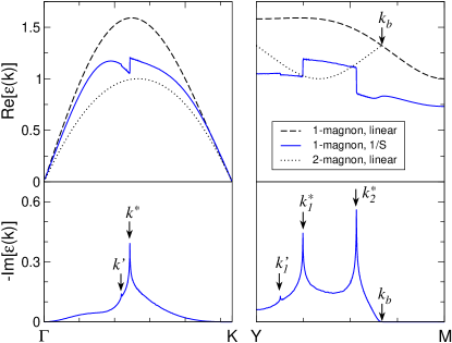
Figure 2: (color online). Upper row: magnon dispersion along the lines $\Gamma$K and YM in the BZ, see Fig. 1. The dashed lines are the LSWT spectrum, the dotted lines is the bottom of the LSWT two-magnon continuum, and the solid lines are the spectrum with the $1/S$ correction. Lower row: imaginary part of the $1/S$ magnon energy along the same lines. $k_{b}$ is the intersection point of the one-magnon branch with the two-magnon continuum along the YM line. $k^{*}$ and $k^{\prime}$ points correspond to the singularities discussed in text.

Decays: long wave-length limit. — The decay vertex (3) for magnons near the $\Gamma$ point scales as $V_{\bf k,Q+q}\!\propto(q^{\prime}-q)\!\sqrt{k/qq^{\prime}}$, for small $q$ and $q^{\prime}\!=\!|{\bf k-q}|$. A simple power counting yields the leading term in the imaginary part of the self-energy. In a typical decay $q,q^{\prime}\!\sim\!k$ giving for the decay probability: $|V_{\bf k,Q+q}|^{2}\!\propto\!k$. Since there is no constraint on the angle between ${\bf k}$ and ${\bf q}$, the 2D phase volume restricted by the energy conservation contributes another factor of $k$, such that $\Im{\rm m}\{\Sigma_{\bf k}(\varepsilon_{\bf k})\}\propto k^{2}$. A more detailed analytical calculation yields $\Im{\rm m}\{\Sigma_{\bf k}(\varepsilon_{\bf k})\}\approx-0.789Jk^{2}$, in agreement with the data in Fig. 2.

The decay vertex for ${\bf k}\!\rightarrow\!{\bf Q}$ magnon has a more conventional scaling: $V_{\bf Q+k,-Q+q}\!\propto\!\sqrt{kqq^{\prime}}$, so the decay probability is $|V|^{2}\!\propto\!k^{3}$. Due to a constraint on the angle between ${\bf k}$ and ${\bf q}$, the decay surface in ${\bf q}$-space is a cigar-shaped ellipse with length $\sim\!k$ and width $\sim\!k^{3/2}$ that makes the restricted phase volume of decays to scale as $k^{1/2}$. This results in a nontrivial $k^{7/2}$ scaling of the decay rate. Numerically, along the $\Gamma$K line $\Im{\rm m}\{\Sigma_{\bf k}(\varepsilon_{\bf k})\}\approx-1.2Jk^{7/2}$. In a similar manner, one can show that at the boundary of decay region (e.g., point $k_{b}$ in Fig. 2) the decay rate grows as $\Im{\rm m}\{\Sigma_{\bf k}(\varepsilon_{\bf k})\}\propto(k-k_{b})^{2}$.

Spectrum: singularities due to decays. — A remarkable feature of the spectrum in Fig. 2 is the singularities in the real and the imaginary parts of $\tilde{\varepsilon}_{\bf k}$. Clearly, they are due to spontaneous decays as it is only the decay term in (4) that contributes to the imaginary part.

A close inspection shows that $k^{\prime}$ and $k^{*}$ singularity points in Fig. 2 correspond exactly to the intersection of $\Gamma$K and YM lines with the saddle-points in the continuum, solid and dashed lines in Fig. 1. The “strong” ($k^{*}$) and “weak” ($k^{\prime}$) singularities correspond to decays into identical and non-identical magnons, solutions (c) and (d) above, respectively. Fig. 3 shows the decay contours, i.e., 1D surfaces in a 2D ${\bf q}$-space into which a magnon with the momentum ${\bf k}$ can decay, for $k^{\prime}$ and $k^{*}$ saddle points along the $\Gamma$K line. In both cases, these contours undergo topological transition.

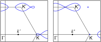
Figure 3: (color online). The upper right parts of the BZ in the ${\bf q}$-space. The decay contours for $k=k^{\prime}$ (left) and $k=k^{*}$ (right) along the $\Gamma$K line are shown. Both ${\bf k}$-points correspond to the saddle points in the two-magnon continuum. The corresponding ${\bf q}$-contours undergo topological transition.

Close to such a transition the denominator in Eq. (4) is expanded as $\varepsilon_{\bf k}\!-E_{{\bf k},{\bf q}}\!\approx\!(v_{1}\!-\!v_{2})\Delta k\!-\!\beta_{x}q_{x}^{2}\!+\!\beta_{y}q_{y}^{2}$, $v_{1}$ and $v_{2}$ are velocities of the initial and final magnons, respectively, $\beta_{i}$ are constants, $\Delta k\!=\!k\!-\!k^{*}$, $k^{*}$ is the saddle point. Integration in Eq. (4) yields a logarithmic singularity in the imaginary part ${\Im}{\rm m}\{\Sigma_{k}\}\propto-\ln|\Lambda/\Delta k|$ and a concomitant finite jump in the real part of the self-energy ${\Re}{\rm e}\{\Sigma_{k}\}\propto{\rm sign}(\Delta k)$, $\Lambda$ is a cutoff. The cutoff (size of the “bubble” in Fig. 3) is small in the case of “weak” singularities, which explains the weakness of them. The logarithmic form agrees perfectly with the data in Fig. 2. Overall, our analysis of the long- and short wave-length behavior gives complete understanding of the $1/S$ results for the magnon spectrum in TLAF.

An important question is whether the singularities in the spectrum will withstand the higher-order treatment. The first possibility is when at least one of the final magnons is itself unstable. Then the log-singularity will be cut off by the decay rate of the final magnon and ${\Im}{\rm m}\{\Sigma_{k}\}$ will have, at most, a weak maximum near the topological transition. For the TLAF such a scenario is realized for a large fraction of the “weak” singularities ($k^{\prime}$ in Fig. 2). However, all of the “strong” singularities ($k^{*}$ in Fig. 2) and some of the “weak” ones belong to another class, in which both magnons created in the decay are stable. We have checked that the first-order $1/S$ corrections do not shift appreciably the instability boundaries in Fig. 1. Hence, at the saddle points, the logarithmic divergence of the one-loop diagrams will persist even for the renormalized spectrum. In such a case, vertex corrections become important pitaevskii . Summation of an infinite series of loop diagrams yields the self-energy from the decay processes near the singular point: $\Sigma_{\bf k}(\omega)\simeq ia/\ln|\Delta\omega-v_{2}\Delta k|$, with $a>0$. One may conclude that the decay rate becomes vanishingly small as $\Delta\omega,\Delta k\rightarrow 0$. This is, however, not true. An attempt to solve the Dyson’s equation $G_{\bf k}^{-1}(\omega)=0$ with this self-energy yields no solution for $\omega$ near the real axis. Therefore, the decay rate of quasiparticles around solid lines in Fig. 1 will remain large and quasiparticle peaks will be strongly suppressed even for large $S$.

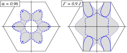
Figure 4: (color online). Decay regions and singularity lines for the $XXZ$ model, $\alpha=0.96$ (left) and the $J-J^{\prime}$ model, $J^{\prime}/J=0.9$ (right). Definition of lines is the same as in Fig. 1.

Other models on a TL. — Two straightforward generalizations of the Heisenberg model on a TL are (i) the anisotropic $XXZ$ model with $\alpha=J_{z}/J_{xy}<1$ and (ii) the $J$–$J^{\prime}$ model for an orthorhombically distorted triangular lattice with one of the interactions within the triangle ($J$) stronger than the other two ($J^{\prime}$).

In the spectrum of the $XXZ$ model magnons at ${\bf Q}$ are gapped with the gap $\varepsilon_{\bf Q}\!\propto\!\sqrt{1-\alpha}$ at $\alpha\!\lesssim\!1$. This has two immediate consequences: (a) magnons at ${\bf k}\rightarrow 0$ are stable up to $\varepsilon_{\bf k}=2\varepsilon_{\bf Q}$ and (b) ${\bf Q}$-magnons become stable themselves. Thus, the star-shaped decay region in Fig. 1 develops a hole in the middle and have vertices shrunk and rounded. The evolution of the decay boundary with $\alpha<1$ is non-trivial. Initially, the emission of a ${\bf Q}$ magnon remains an absolute minimum of the two-magnon continuum for most of the decay region. At $\alpha_{1}\!\approx\!0.993$ the decay into non-equivalent magnons switches from being a line of saddle points into the absolute minima of the continuum and takes over the decay boundary. Fig. 4 shows the instability and the singularity lines for a representative value $\alpha=0.96$. Further decrease of $\alpha$ completely eliminates the decay region at around $\alpha\approx 0.92$. Thus, magnon decays are present in an anisotropic TLAF, but only at not too large anisotropies.

For the $J$–$J^{\prime}$ model the Goldstone modes at ${\bf k}=\pm{\bf Q}$ are preserved but the ordering wave-vector ${\bf Q}$ becomes incommensurate. This does not change the kinematics of the decays for the ${\bf k}\rightarrow 0$ magnons, but forbids the decays from the vicinity of the ${\bf Q}$ point into the vicinity of $-{\bf Q}$ point as the quasi-momentum cannot be conserved. However, the decays in the vicinity of (inequivalent now) K’ points are still allowed. Overall, the decay region grows with the decrease of $J^{\prime}$. At $J^{\prime}\approx 0.34J$, relevant to Cs₂CuCl₄ Coldea , the decay region covers most of the BZ. With the decrease of $J^{\prime}$ the LSWT single-magnon dispersion develops a low-energy branch in the direction perpendicular to the “strong” $J$. That makes the rest of the spectrum prone to decays into it.

Conclusions. — We have shown that magnon decays must be prominent in a wide class of noncollinear AFs. We calculated the decay rate in the spin-1/2 TLAF within the spin-wave theory. In the long-wavelength limit, the life-time of low-energy excitations is predicted to exhibit a non-trivial scaling. For the short-wavelength magnons, the decay rate is large, $2\Im{\rm m}\{\tilde{\varepsilon}_{\bf k}\}\sim 0.4\Re{\rm e}\{\tilde{\varepsilon}_{\bf k}\}$, in a substantial part of the BZ. Topological transitions of the decay surface also lead to strong singularities in the spectrum that remain essential even for large values of spin. Therefore, excitations in ordered, spin-$S$, AFs may not necessarily be well-defined for all wave-vectors.

Acknowledgments. — We are indebted to O. Starykh for illuminating discussions and sharing his unpublished work. This work was supported by DOE under grant DE-FG02-04ER46174 (A.L.C.).

References

- (1) J. M. Ziman, Electrons and phonons, (Oxford University Press, Oxford, 1960).
- (2) L. P. Pitaevskii, Zh. Éksp. Teor. Fiz. 36, 1168 (1959) [Sov. Phys. JETP 9, 830 (1959)].
- (3) F. J. Dyson, Phys. Rev. 102, 1217 (1956); A. B. Harris et al., Phys. Rev. 3, 961 (1971).
- (4) A. I. Akhiezer, V. G. Bar’yakhtar, S. V. Peletminskii, Spin waves (North-Holland, Amsterdam, 1968).
- (5) S. J. Miyake, Prog. Theor. Phys. 73, 18 (1985); J. Phys. Soc. Jpn. 61, 983 (1992).
- (6) T. Ohyama and H. Shiba, J. Phys. Soc. Jpn. 62, 3277 (1993).
- (7) A. V. Chubukov et al., J. Phys. Condens. Matter 6, 8891 (1994).
- (8) M. E. Zhitomirsky and T. Nikuni, Phys. Rev. B 57, 5013 (1998).
- (9) M. E. Zhitomirsky and A. L. Chernyshev, Phys. Rev. Lett. 82, 4536 (1999).
- (10) W. Zheng et al., Phys. Rev. Lett. 96, 057201 (2006).
- (11) O. A. Starykh et al., Phys. Rev. B 74, 180403(R) (2006).
- (12) R. Coldea et al., Phys. Rev. Lett. 86, 1335 (2001).