Augmented orbital minimization method for linear scaling electronic structure calculations

Abstract

We present a novel algorithm which can overcome the drawbacks of the conventional linear scaling method with minimal computational overhead. This is achieved by introducing additional constraints, thus eliminating the redundancy of the orbitals. The performance of our algorithm is evaluated in ab initio molecular-dynamics simulations as well as in a model system.

1 INTRODUCTION

Electronic structure calculations often provide very accurate physical and chemical properties of various microscopic systems from first principles, which makes them attractive to experimentalists as well as theoreticians [1, 2, 3, 4, 5]. However, the computational cost of such calculations grows cubically (or faster) with the number of atoms in the system, thereby limiting the maximum number of atoms to $\approx 10^{3}$ on today’s computers. Therefore, much effort has been devoted to the development of so-called linear scaling methods, whose computational cost grows only linearly with system size [5, 6, 7, 8], usually by making some assumptions about the electronic structure of the system [9].

The emergence of the linear scaling methods has also promoted the development of various discretization schemes in real space in the last decade [10, 11, 12, 13], such as finite difference and finite element methods. These real space methods are considered more appropriate for linear scaling methods than plane waves, because they can easily take advantage of the localization of electrons [9] while retaining systematic convergence. Alternatively, the use of atomic basis set in linear scaling methods is also an attractive approach [14, 7, 15, 16].

From the point of view of computational cost, the orbital minimization method (OMM) [17, 18, 19, 20], which is designed for nonmetallic systems, is among the most promising linear scaling algorithms proposed so far. Moreover, OMM is easy to implement, and is able to deal with nonorthogonal basis functions without much difficulty. Therefore, much work has been carried out on the implementation of OMM, including first-principles calculations using real-space methods [25, 26, 27, 21, 22, 23, 24]. Unfortunately, if localization constraints are imposed on the orbitals to achieve linear scaling, a naive implementation of OMM suffers from several drawbacks [6], which has discouraged the use of OMM in realistic applications to date. In the present paper, we propose a simple yet effective algorithm which can overcome the drawbacks of OMM when the electronic structure of the system is qualitatively predictable.

2 ALGORITHM

First of all, we briefly describe the basic formalism of electronic structure calculations here. For notational simplicity, only non-self-consistent problems are considered here, but extention to self-consistent ones is straightforward. Moreover, we assume that the orbitals are real, and that there is no spin degeneracy. We also assume the presence of an energy gap between the occupied and unoccupied states throughout the paper. Then, the conventional total energy functional $\widetilde{E}_{\mbox{\scriptsize total}}$ is given by

$$\widetilde{E}_{\mbox{\scriptsize total}}[\widetilde{\psi}]=\sum_{i=1}^{N}\widetilde{H}_{ii},$$ (1)

where the Hamiltonian ${\cal H}=-\nabla^{2}+{\cal V}$, $\widetilde{H}_{ii}=<\!\widetilde{\psi}_{i}\,|\,{\cal H}\,|\,\widetilde{\psi}_{i}\!>$, ${\cal V}$ is the potential felt by the electrons, and $N$ is the number of occupied orbitals [28]. If $\widetilde{E}_{\mbox{\scriptsize total}}$ is minimized with repect to the orbitals $\{\widetilde{\psi}_{i}(\mbox{\boldmath$r$})\}_{i=1}^{N}$ under the orthonormality constraints

$$<\!\widetilde{\psi}_{i}\,|\,\widetilde{\psi}_{j}\!>=\delta_{ij},$$ (2)

$\widetilde{E}_{\mbox{\scriptsize total}}$ and $\{{\widetilde{\psi}_{i}}\}$ will converge to the sum of the $N$ lowest eigenvalues of ${\cal H}$ and corresponding eigenstates, respectively, except for the degrees of freedom associated with any unitary transformation. This redundancy can be exploited to construct the maximally localized Wannier functions (MLWFs) [29, 30], whose spread in real space,

$$\Omega=\sum_{i=1}^{N}(<\!r^{2}\!>_{i}-<\!r\!>_{i}^{2}),$$

is minimum among all states given by the unitary transformation of the eigenstates. An efficient calculation of MLWFs along the trajectory of Car-Parrinello dynamics is also an active area of research [31, 32, 33, 34]. In the following, MLWFs are denoted by $\{w_{i}(\mbox{\boldmath$r$})\}_{i=1}^{N}$.

On the other hand, the generalized total energy functional [35, 36, 17, 37] used in OMM is given by

$$E_{\mbox{\scriptsize total}}[{\psi}]=\sum_{i,j=1}^{N}(S^{-1})_{ij}\cdot H_{ij},$$ (3)

where $H_{ij}=<\!\psi_{i}\,|\,{\cal H}\,|\,\psi_{j}\!>$, and the overlap matrix $S$ is defined by $S_{ij}=<\!\psi_{i}\,|\,\psi_{j}\!>$. The minimum value of $E_{\mbox{\scriptsize total}}$ agrees with that of $\widetilde{E}_{\mbox{\scriptsize total}}$, and $\{\psi_{i}\}$ that minimize $E_{\mbox{\scriptsize total}}$ are nonorthogonal functions that span the same subspace as the $N$ lowest eigenstates of ${\cal H}$. While there are several variants of this functional [18, 19, 20] which rely on the Neumann expansion of $S^{-1}$, we will not go into detail here. In analogy with the case of $\widetilde{E}_{\mbox{\scriptsize total}}$, $E_{\mbox{\scriptsize total}}$ is invariant under the linear transformation

$$|\,\psi_{i}\!>=\sum_{j}X_{ij}|\,\psi^{\prime}_{j}\!>$$ (4)

for any nonsingular matrix $X$ of size $N$. Therefore, attempts have been made to construct nonorthogonal localized orbitals (NOLOs), which can be more localized than MLWFs by taking advantage of the higher degree of freedom [38, 39, 40]. However, special attention has to be paid to the risk of falling into linearly dependent states while constructing NOLOs.

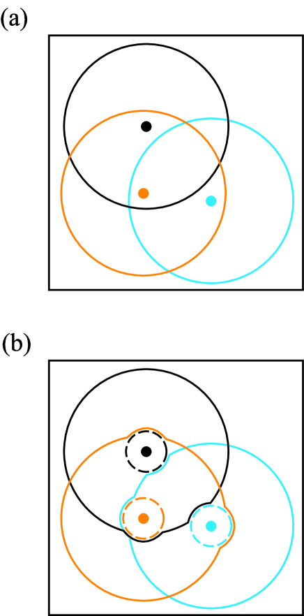
Figure 1: (a) Conventional definition of the localization regions in OMM (solid lines). Filled circles denote the centers of localization, which are usually either atomic positions or bond centers. (b) Localization regions in AOMM. Kernel regions are shown with dashed lines.

In order to achieve linear scaling with the OMM, localization constraints are imposed on the orbitals (Fig.1 (a)) during the minimization of $E_{\mbox{\scriptsize total}}$ [17]. When each orbital is strictly localized within a given region of space, called the localization region (LR), $S$ and $H$ would be sparse matrices, and the computational cost of evaluating each nonzero element of $S$ and $H$ would be independent of system size [41]. Therefore, $E_{\mbox{\scriptsize total}}$ as well as its gradient can be calculated with linear scaling in a straightforward manner [42]. Moreover, the optimized orbitals are expected to be good approximations to MLWFs, which are least likely to be influenced by the localization constraints among the unitary transformation of the ground state. Therefore, the centers of LRs are usually chosen as close to those of MLWFs as possible.

Unfortunately, in the presence of localization constraints, iterative minimization of the total energy becomes extremely difficult [6], often requiring hundreds or thousands of iterations to converge. Furthermore, the orbitals can be trapped at local minima during the minimization process [6, 27, 19], which results in poor conservation of the total energy in molecular-dynamics simulations. The major source of these problems is that $E_{\mbox{\scriptsize total}}$ has a pathological shape around the minimum, which arises from the fact that $E_{\mbox{\scriptsize total}}$ is only approximately invariant under the linear transformation of Eq.(4) in the presence of localization constraints [6, 43].

While much effort has been made to overcome these problems [6, 19, 44], the performance and reliability of OMM under the localization constraints still appear to be insufficient for routine use in realistic applications. In the following, we present a simple prescription to make OMM a practical linear scaling algorithm with minimal computational overhead. To this end, we introduce here the concept of kernel region (KR), which plays an important role in the algorithm explained below. For simplicity, we assume that only one orbital is assigned to each LR, but extension to the multi-orbital case is straightforward. Then, KRs of a given system are generated under the following conditions:

1. Each LR includes its own KR, which preferably includes the center of a MLWF.

2. There is no overlap between any two KRs.

3. No partial overlap between any LR and KR is allowed.

An example of a set of LRs and KRs that satisfy these conditions is shown in Fig.1 (b). In practice, we first generate LRs and KRs temporarily, e.g. by the distance criterion, that satisfy conditions (a) and (b). Then, if more(less) than a given fraction (say, 40 %) of each KR is included in some other LR, the border of that LR is modified to include(exclude) the KR completely, thus satisfying condition (c). Since KRs are usually much smaller than LRs, these modifications will not have a significant impact on the shape of LRs. In the following, LRs and KRs that satisfy the above conditions are denoted by $\{L_{i}\}_{i=1}^{N}$ and $\{K_{i}\}_{i=1}^{N}$, respectively.

We now define the kernel functions $\{\chi_{i}(\mbox{\boldmath$r$})\}_{i=1}^{N}$ that have the following properties:

1. $\chi_{i}(\mbox{\boldmath$r$})$ approximates $w_{i}(\mbox{\boldmath$r$})$ when $\mbox{\boldmath$r$}\in K_{i}$.

2. $\chi_{i}(\mbox{\boldmath$r$})=0$ when $\mbox{\boldmath$r$}\notin K_{i}$.

3. $<\!\chi_{i}\,|\,\chi_{i}\!>=1$.

Therefore, $<\!\chi_{i}\,|\,\chi_{j}\!>=\delta_{ij}$ is satisfied automatically.

In the augmented orbital minimization method (AOMM), $E_{\mbox{\scriptsize total}}$ is minimized with respect to the localized orbitals $\{\psi_{i}\}$ under the additional constraints that

$$<\!\chi_{j}\,|\,\psi_{i}\!>=0$$ (5)

for any $j\neq i$, where $i,j=1,2,\cdots N$. The role of these constraints is to orthogonalize $\psi_{i}(\mbox{\boldmath$r$})$ approximately to $w_{j}(\mbox{\boldmath$r$})$ for any $j\neq i$, in the hope that $\psi_{i}(\mbox{\boldmath$r$})$ will be a good approximation to $w_{i}(\mbox{\boldmath$r$})$ at the minimum. Eq.(5) is satisfied by an explicit orthogonalization as

$$|\,\psi_{i}^{\prime}\!>=\hat{P}_{i}|\,\psi_{i}\!>=|\,\psi_{i}\!>-\sum_{j\neq i}|\,\chi_{j}\!><\!\chi_{j}\,|\,\psi_{i}\!>,$$ (6)

where the projection operator is given by

$$\hat{P}_{i}=I-\sum_{j\neq i}|\,\chi_{j}\!><\!\chi_{j}\,|.$$ (7)

Summation with respect to $j$ should be taken only if $K_{j}\in L_{i}$, because $<\!\chi_{j}\,|\,\psi_{i}\!>\equiv 0$ otherwise. Therefore, the computational cost of projection is relatively minor, scaling only linearly with system size. Note that if $\psi_{i}(\mbox{\boldmath$r$})$ is localized within $L_{i}$, so is $\psi_{i}^{\prime}(\mbox{\boldmath$r$})$ due to the properties of KRs and kernel functions. Moreover, each orbital remains unchanged inside its own KR after the projection, i.e. $\psi_{i}^{\prime}(\mbox{\boldmath$r$})=\psi_{i}(\mbox{\boldmath$r$})$ if $\mbox{\boldmath$r$}\in K_{i}$.

There is no unique way to define the kernel functions for given KRs, but if those KRs are used as the LRs in the conventional OMM, the optimized orbitals will serve as the kernel functions. These are called static kernel functions, since they do not change during the electronic structure calculations. Note that there is no slow convergence or local minima problem when the LRs do not overlap. An alternative way to define the kernel functions is to use a mask function $m_{i}(\mbox{\boldmath$r$})$, such that $m_{i}(\mbox{\boldmath$r$})=1$ when $\mbox{\boldmath$r$}\in K_{i}$ and $m_{i}(\mbox{\boldmath$r$})=0$ otherwise [45]. Then, if the orbitals are reasonably close to the ground state, $\{m_{i}(\mbox{\boldmath$r$})\psi_{i}(\mbox{\boldmath$r$})\}_{i=1}^{N}$ can be used as the kernel functions after normalization. We call them dynamic kernel functions, because they are updated at every step of the minimization.

When the kernel functions do not depend on the orbitals, the gradient of $E_{\mbox{\scriptsize total}}$ under the constraints of Eq.(5) is given by

$$|\,g_{i}\!>=\hat{P}_{i}\,\frac{\partial E_{\mbox{\scriptsize total}}}{\partial\psi_{i}},$$ (8)

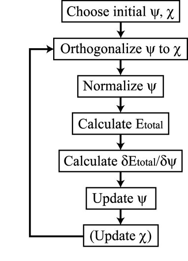
Figure 2: Flow chart of AOMM for a given ionic configuration. The loop is repeated until a convergence criterion is satisfied. Update of $\chi$ can be skipped if static kernel functions are used.

which can also be evaluated with linear scaling effort. If dynamic kernel functions are used, a correction term is required to take into account the dependence of $\{\chi_{i}\}$ on $\{\psi_{i}\}$, which, however, can be calculated in a straightforward manner. Fig.2 shows the flow chart of the electronic structure calculation for a given ionic configuration in the AOMM.

3 RESULTS

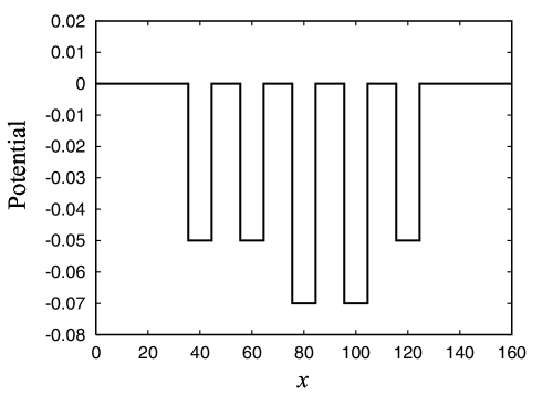
Figure 3: Five square potential wells of widths 9 are centered at 40,60,80,100, and 120.

The performance of our algorithm is first evaluated in a simple one-dimensional problem. We consider a system consisting of 5 electrons in the potential wells shown in Fig.3, where $x=0,1,\cdots,160$, and vanishing boundary conditions are imposed on the orbitals. When a 3-point finite-difference approximation is used for the Laplacian, the Hamiltonian ${\cal H}$ is given by a tridiagonal matrix of size 161$\times$161 as

$${\cal H}=\left(\begin{array}[]{ccccc}2+v_{0}&-1&&&\\ -1&2+v_{1}&-1&&\\ &\ldots&\ldots&\ldots&\\ &&-1&2+v_{159}&-1\\ &&&-1&2+v_{160}\\ \end{array}\right).$$ (9)

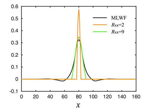
Figure 4: MLWF and kernel functions which belong to the central KR.

We used 5 pairs of LRs and KRs centered at 40, 60, 80, 100, and 120, the radii of which are denoted by $R_{\mbox{\tiny LR}}$ and $R_{\mbox{\tiny KR}}$, respectively. Therefore, each LR(KR) is given 2$R_{\mbox{\tiny LR}}$+1 (2$R_{\mbox{\tiny KR}}$+1) degrees of freedom. It is worth noting that in this system the conditions (a)-(c) given in the previous section translate into the inequalities as follows: (a) $R_{\mbox{\tiny KR}}\leq R_{\mbox{\tiny LR}}$, (b) $0\leq R_{\mbox{\tiny KR}}\leq 9$, and (c) $20-R_{\mbox{\tiny KR}}\leq R_{\mbox{\tiny LR}}<20+R_{\mbox{\tiny KR}},40-R_{\mbox{\tiny KR}}\leq R_{\mbox{\tiny LR}}<40+R_{\mbox{\tiny KR}},\cdots$ are not allowed. The centers of the MLWFs constructed from the 5 lowest eigenstates of ${\cal H}$ are given by (39.66, 60.02, 80.03, 99.98, 120.27), which justify our choice of LRs and KRs. We used static kernel functions which were calculated in advance, as explained in the previous section. The kernel functions which belong to the central KR are compared with the MLWF in Fig. 4.

The ground state of this system was calculated iteratively by the conjugate gradient method [46] with no preconditioning. Ground state calculations were repeated 100 times from different random initial states [47], from which statistics were collected. Each calculation was terminated successfully when the total energy difference between two successive steps was smaller than $10^{-11}$. If convergence was not achieved after 1000 iterations, the calculation was regarded as a failure, which was excluded from the statistics.

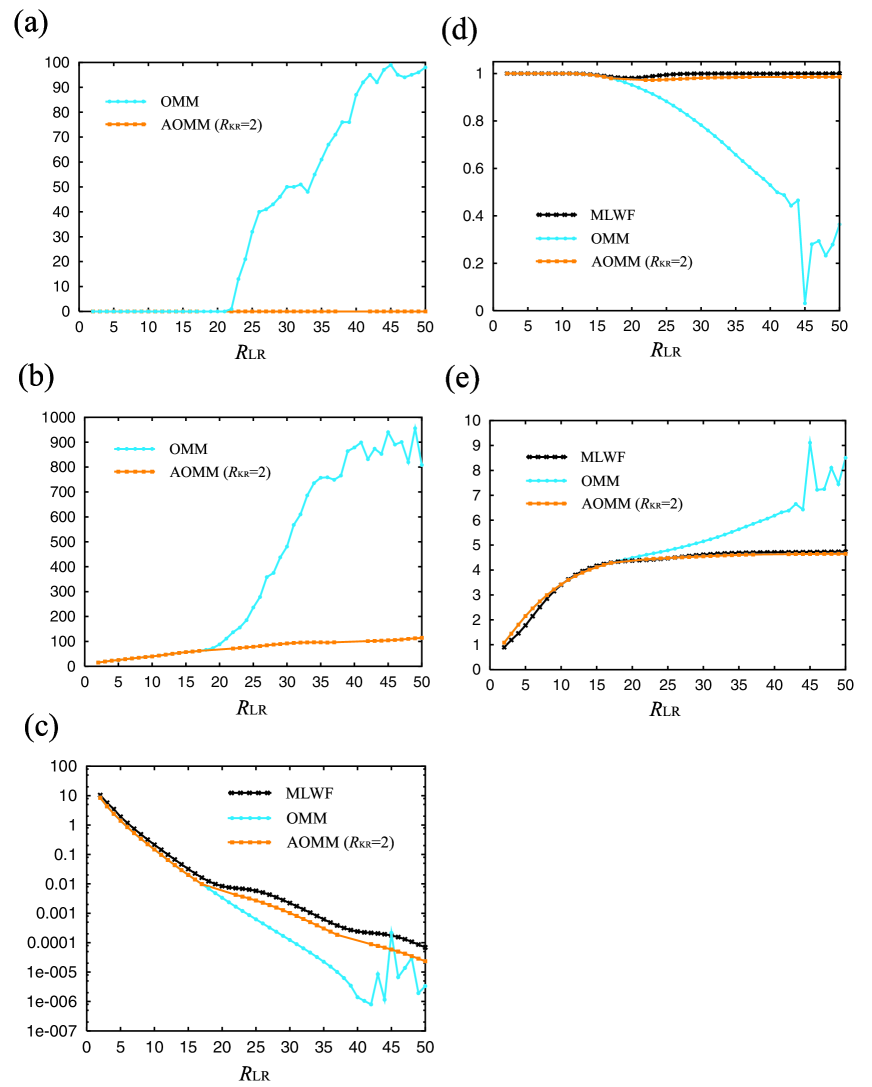
Figure 5: (a) Number of unsuccessful calculations. (b) Average number of iterations. (c) Relative errors in total energy. (d) Determinant of the overlap matrix. (e) Average spread of the orbitals.

Fig.5 (a) shows the number of unsuccessful calculations as functions of $R_{\mbox{\tiny LR}}$ for the OMM and AOMM. For small values of $R_{\mbox{\tiny LR}}$, where only a small portion of the neighboring LRs overlap, both methods work equally well. In the OMM, however, this number grows rapidly as the LRs begin to include the centers of neighboring LRs at $R_{\mbox{\tiny LR}}\approx 20$, and the iterations almost always fail to converge when the second nearest neighbors are also included at $R_{\mbox{\tiny LR}}\approx 40$. In contrast, no failure is observed in the AOMM for all values of $R_{\mbox{\tiny LR}}$, which clearly demonstrates the advantage of AOMM over the OMM.

Average number of iterations for OMM (Fig.5 (b)) shows a similar tendency. While the convergence rate also slowly deteriorates with $R_{\mbox{\tiny LR}}$ in the AOMM, this problem is easily overcome by a suitable preconditioner and/or the multigrid method [10].

Fig.5 (c) shows the relative errors in total energy from the exact value obtained by diagonalization of ${\cal H}$. For comparison, we also show the values for the MLWFs, which are first projected onto the LRs of size $R_{\mbox{\tiny LR}}$, followed by smoothing at the boundaries. While the OMM gives the fastest convergence with respect to $R_{\mbox{\tiny LR}}$, the errors saturate at $R_{\mbox{\tiny LR}}\approx 40$, because the optimization is always trapped at local minima. In contrast, no saturation is observed in the results of AOMM, even if the convergence is slower due to the additional constraints of Eq.(5). Overall, AOMM values are very close to those of MLWFs, including the slowdown at $R_{\mbox{\tiny LR}}\approx 20$ and $40$, but converge somewhat faster. Moreover, no local minima were found in the AOMM.

The determinant of the overlap matrix $S$ at the ground state is shown in Fig.5 (d). While AOMM and MLWF behave similarly, the asymptotic value of AOMM ($\approx$ 0.986) is slightly smaller than that of MLWF (=1). In contrast, OMM values keep decreasing with $R_{\mbox{\tiny LR}}$, which implies that the orbitals are falling into linearly dependent states.

Fig.5 (e) shows the average spread $\sigma$ of the orbitals, where $\sigma=\sum_{i=1}^{N}(<\!x^{2}\!>_{i}-<\!x\!>_{i}^{2})^{\frac{1}{2}}/N$. Although AOMM and MLWF give very similar results, OMM values increase steadily with $R_{\mbox{\tiny LR}}$, which suggests that the orbitals deviate from the picture of MLWFs at large $R_{\mbox{\tiny LR}}$.

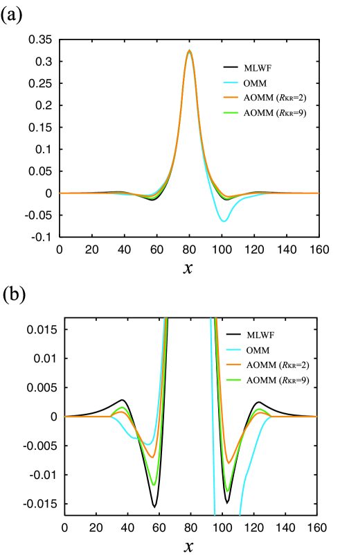
Figure 6: (a) Localized orbitals which belong to the central LR ($R_{\mbox{\tiny LR}}=50$), obtained from OMM and AOMM ($R_{\mbox{\tiny KR}}$=2 and 9)). (b) Enlarged view of (a).

To promote further understanding of this point, the optimized orbitals which belong to the central LR are compared with the MLWF in Fig.6. A prominent feature of the MLWF is the oscillatory behavior at large distances from the center, called the orthogonalization tail [40], which arises from the orthogonality constraints of Eq.(2). While the orbitals obtained from AOMM are very similar to the MLWF, they decay faster at large distances, particularly when $R_{\mbox{\tiny KR}}$ is small. In contrast, the orbital from OMM exhibits irregular behavior, as expected from the large $\sigma$ mentioned above.

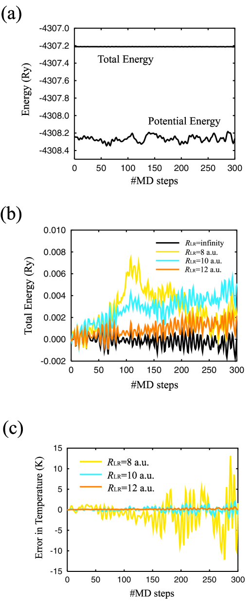
Figure 7: (a) Time evolution of the total energy and the ionic potential energy when all orbitals are extended. (b) Conservation of the total energy during the simulations. Total energy of the initial configuration is chosen as the origin for each run. (c) Errors in ionic temperature during the simulations.

We have also implemented AOMM in our first-principles code FEMTECK (Finite Element Method based Total Energy Calculation Kit) [48, 21] to assess its performance under realistic conditioins. We have carried out ab initio molecular-dynamics simulations of liquid water at ambient conditions using a cubic supercell of side 29.35 Bohr containing 125 molecules. All hydrogen atoms in the system were given the mass of deuterium, and a timestep of 40 a.u. ($\sim$ 0.97 fs) was used in all simulations. We used 125 pairs of LRs and KRs, all of which are centered at the oxygen atoms, and 4 orbitals were assigned to each LR and KR. The orbitals were optimized using a limited-memory variant of the quasi-Newton method [49, 50, 51] with a tolerance of $2\times 10^{-10}$ Ry/orbital. Other details of the simulations are described in our recent publications [52, 53]. Table 1 shows the details of 4 runs, where dynamic kernel functions were used in all AOMM runs [54]. Fig. 7(a) shows the time evolution of the total energy and potential energy for extended orbitals, which proves the accuracy of the ionic forces in our simulations. Fig.7(b) and (c) show the total energies and errors in ionic temperature during the molecular-dynamics simulations. Ionic forces were calculated under the assumption that all LRs and KRs are fixed in space. In reality, neither assumption is true, which explains the irregular behavior of the total energies when $R_{\mbox{\tiny LR}}$ is small. However, conservation of the total energy for $R_{\mbox{\tiny LR}}=12$ Bohr is already competitive with that of the extended orbitals. The ionic temperature in the OMM run is also reproduced with an error of $<$ 1 K when $R_{\mbox{\tiny LR}}=12$ Bohr.

4 DISCUSSION

In this section, we make several observations on the properties of AOMM.

When all LRs are extended, each LR will include all the KRs. In this case, Eq.(5) imposes $N^{2}-N$ constraints, which is equivalent to the number of degrees of freedom associated with Eq.(4) (assuming that each orbital is normalized). Therefore, the ground state of the system is uniquely determined (except for sign) with no loss of accuracy, since the redundancy of the orbitals is completely removed. If the LRs have a finite size smaller than the unit cell, $E_{\mbox{\scriptsize total}}$ is no longer invariant under the transformation of Eq.(4). Nevertheless, if a large portion of two LRs overlap with each other, $E_{\mbox{\scriptsize total}}$ would be nearly invariant under the mixing of two orbitals which belong to these LRs. This near-redundancy is considered the major source of slow convergence and local minima problem [6, 43]. If these LRs are denoted by $L_{1}$ and $L_{2}$, we can expect that $K_{1}\in L_{2}$ and $K_{2}\in L_{1}$, since the KRs are located near the centers of LRs. Then, Eq.(5) gives two constraints on these orbitals, which can eliminate the near-redundancy associated with $L_{1}$ and $L_{2}$. On the other hand, if only a small portion of $L_{1}$ and $L_{2}$ overlap, they do not cause any problems, as shown in the previous section. Therefore, the above observation for the extended orbitals remains essentially valid even if the orbitals are localized.

In the limiting case of large (yet nonoverlapping) KRs, the static kernel functions will be rather good approximations to the MLWFs. If the kernel functions are regarded as the zeroth-order approximation to the ground state, the orbitals can be written as follows:

$$|\,\psi_{i}\!>=|\,\chi_{i}\!>+|\,\delta\psi_{i}\!>.$$ (10)

Then, the constraints of Eq.(5) would be equivalent to

$$<\!\chi_{j}\,|\,\delta\psi_{i}\!>=0,$$ (11)

which is in close analogy with the case of perturbation theory [55, 56]. Note, however, that our calculations are fully self-consistent. On the other hand, if the precise positions of MLWF centers are known a priori, e.g. in perfect crystals, the KRs can be chosen infinitesimally small, in which case each kernel function would be a $\delta$-function. Then, Eq.(5) reduces to $\psi_{i}(\mbox{\boldmath$r$}_{j})=0$, where $\mbox{\boldmath$r$}_{j}$ denotes the position of $K_{j}$. Since we can expect that $\psi_{i}(\mbox{\boldmath$r$}_{i})\neq 0$ for any $i$, these constraints will guarantee the linear independence of the orbitals. While it may seem counterintuitive, the total energy is systematically lower for smaller KRs, if each KR is chosen appropriately. This is explained as follows. When KRs are large, the ground state orbitals resemble the conventional MLWFs, which suffer from large orthogonalization tails. As the KRs become smaller, the influence of Eq.(5) becomes more local, thus reducing the orthogonalization tails of the orbitals. Therefore, from the point of view of minimizing the errors in total energy for given LRs, the KRs should be chosen as small as possible.

So far, we have implicitly assumed that the positions of MLWFs centers, which are required for the determination of KRs and LRs, are known a priori with sufficient accuracy. Fortunately, in many systems with large energy gaps, e.g. in liquid water, the electrons form a closed shell. Then, approximate positions of MLWF centers are available based solely on the knowledge of chemistry. If, however, part of the system consists of complex atomic configurations with unknown electronic structures, it would be difficult to choose the KRs and LRs appropriately. One possible solution to this problem is the implementation of the adaptive localization centers [26, 27], which gives approximate positions of MLWF centers without a priori knowledge of the system. An alternative approach is to use extended LRs for the orbitals, the behavior of which is unpredictable. This problem will be discussed in more detail in future publications.

5 CONCLUSION

In this article, we have shown that the linear scaling method based on OMM can be as robust as the conventional algorithm using extended orbitals, when augmented with additional constraints to guarantee linear independence of the orbitals. Although it is difficult to give a general proof, AOMM appears to overcome the slow convergence and local minima problem of OMM, provided that LRs, KRs, and kernel functions are chosen appropriately. A more detailed study on the performance of AOMM in molecular-dynamics simulations is under way, and will be reported in a forthcoming paper.

Table 1: Simulation details for each run. $M$ and $\Delta E$ denote the average number of iterations and the error in total energy for the initial configuration, respectively.

	Method	$R_{\mbox{\tiny LR}}$ (Bohr)	$R_{\mbox{\tiny KR}}$ (Bohr)	$M$	$\Delta E$ (Ry)
(a)	OMM	$\infty$	–	12.0	0
(b)	AOMM	8	0.8	14.1	0.13456
(c)	AOMM	10	0.8	14.8	0.02040
(d)	AOMM	12	0.8	14.9	0.00309

References

- [1] P. Hohenberg and W. Kohn: Phys. Rev. 136 (1964) B864.
- [2] W. Kohn and L. J. Sham: Phys. Rev. 140 (1965) A1133.
- [3] R. Car and M. Parrinello: Phys. Rev. Lett. 55 (1985) 2471.
- [4] M. E. Tuckerman: J. Phys. Condens. Matter 14 (2002) R1297.
- [5] R. M. Martin: Electronic Structure: Basic Theory and Practical Methods (Cambridge University Press, New York, 2004).
- [6] S. Goedecker: Rev. Mod. Phys. 71 (1999) 1085.
- [7] G. E. Scuseria: J. Phys. Chem. A 103 (1999) 4782.
- [8] S. Y. Wu and C. S. Jayanthi: Phys. Rep. 358 (2002) 1.
- [9] W. Kohn: Phys. Rev. Lett. 76 (1996) 3168.
- [10] T. L. Beck: Rev. Mod. Phys. 72 (2000) 1041.
- [11] J. E. Pask and P. A. Sterne: Modelling Simul. Mater. Sci. Eng. 13 (2005) R71.
- [12] T. Torsti, T. Eirola, J. Enkovaara, T. Hakala, P. Havu, V. Havu, T. Höynälänmaa, J. Ignatius, M. Lyly, I. Makkonen, T. Rantala, J. Ruokolainen, K. Ruotsalainen, E. Räsänen, H. Saarikoski and M. J. Puska: Phys. Stat. Sol. B 243 (2006) 1016.
- [13] K. Hirose, T. Ono, Y. Fujimoto, and S. Tsukamoto: First-Principles Calculations in Real-Space Formalism (Imperial College Press, London, 2005).
- [14] W. Yang: Phys. Rev. Lett. 66 (1991) 1438.
- [15] K. Kitaura, E. Ikeo, T. Asada, T. Nakano, and M. Uebayasi: Chem. Phys. Lett. 313 (1999) 701.
- [16] T. Ozaki and H. Kino: Phys. Rev. B 69 (2004) 195113.
- [17] G. Galli and M. Parrinello: Phys. Rev. Lett. 69 (1992) 3547.
- [18] F. Mauri and G. Galli: Phys. Rev. B 50 (1994) 4316.
- [19] J. Kim, F. Mauri, and G. Galli: Phys. Rev. B 52 (1995) 1640.
- [20] P. Ordejn, D. A. Drabold, R. M. Martin, and M. P. Grumbach: Phys. Rev. B 51 (1995) 1456.
- [21] E. Tsuchida and M. Tsukada: J. Phys. Soc. Jpn. 67 (1998) 3844.
- [22] D. Raczkowski, C. Y. Fong, P. A. Schultz, R. A. Lippert, and E. B. Stechel: Phys. Rev. B 64 (2001) 155203.
- [23] J. J. Mortensen and M. Parrinello: J. Phys. Condens. Matter 13 (2001) 5731.
- [24] F. Shimojo, R. K. Kalia, A. Nakano, and P. Vashishta, Comp. Phys. Commun. 140 (2001) 303.
- [25] J. -L. Fattebert and J. Bernholc, Phys. Rev. B 62 (2000) 1713.
- [26] J. -L. Fattebert and F. Gygi, Comp. Phys. Commun. 162 (2004) 24.
- [27] J. -L. Fattebert and F. Gygi, Phys. Rev. B 73 (2006) 115124.
- [28] No unoccupied states are used throughout the paper.
- [29] N. Marzari and D. Vanderbilt: Phys. Rev. B 56 (1997) 12847.
- [30] G. Berghold, C. J. Mundy, A. H. Romero, J. Hutter, and M. Parrinello: Phys. Rev. B 61 (2000) 10040.
- [31] M. Sharma, Y. Wu, and R. Car: Int. J. Quantum Chem. 95 (2003) 821.
- [32] J. W. Thomas, R. Iftimie, and M. E. Tuckerman: Phys. Rev. B 69 (2004) 125105.
- [33] R. Iftimie, J. W. Thomas, and M. E. Tuckerman: J. Chem. Phys. 120 (2004) 2169.
- [34] B. Kirchner and J. Hutter: J. Chem. Phys. 121 (2004) 5133.
- [35] I. Stich, R. Car, M. Parrinello, and S. Baroni: Phys. Rev. B 39 (1989) 4997.
- [36] T. A. Arias, M. C. Payne, and J. D. Joannopoulos: Phys. Rev. Lett. 69 (1992) 1077.
- [37] R. D. King-Smith and D. Vanderbilt: Phys. Rev. B 49 (1994) 5828.
- [38] S. Liu, J. M. Pérez-Jordá, and W. Yang: J. Chem. Phys. 112 (2000) 1634.
- [39] H. Feng, J. Bian, L. Li, and W. Yang: J. Chem. Phys. 120 (2004) 9458.
- [40] F. A. Reboredo and A. J. Williamson: Phys. Rev. B 71 (2005) 121105.
- [41] We assume that the size of LRs does not increase with system size.
- [42] A small O() overhead is required to invert the overlap matrix , which is minor in realistic calculations.
- [43] D. R. Bowler and M. J. Gillan: Mol. Sim. 25 (2000) 239.
- [44] U. Stephen, D. A. Drabold, and R. M. Martin, Phys. Rev. B 58 (1998) 13472.
- [45] Of course, a smoother function may be used to avoid discontinuities at the boundaries.
- [46] W. H. Press, S. A. Teukolsky, W. T. Vetterling, and B. P. Flannery: Numerical Recipes in Fortran (Cambridge University Press, Cambridge, 1992).
- [47] The initial orbitals were normalized, but not orthogonalized.
- [48] E. Tsuchida and M. Tsukada: Phys. Rev. B 54 (1996) 7602.
- [49] D. C. Liu and J. Nocedal: Math. Prog. 45 (1989) 503.
- [50] P. E. Gill and M. W. Leonard: SIAM J. Optim. 14 (2003) 380.
- [51] E. Tsuchida: J. Phys. Soc. Jpn. 71 (2002) 197.
- [52] E. Tsuchida: J. Chem. Phys. 121 (2004) 4740.
- [53] E. Tsuchida: J. Phys. Soc. Jpn. 75 (2006) 054801.
- [54] We were able to achieve satisfactory convergence with OMM only when .
- [55] A. Putrino, D. Sebastiani, and M. Parrinello: J. Chem. Phys. 113 (2000) 7102.
- [56] D. M. Benoit, D. Sebastiani, and M. Parrinello: Phys. Rev. Lett. 87 (2001) 226401.