Accumulating Particles at the Boundaries of a Laminar Flow

Abstract

The accumulation of small particles is analyzed in stationary flows through channels of variable width at small Reynolds number. The combined influence of pressure, viscous drag and thermal fluctuations is described by means of a Fokker-Planck equation for the particle density. It is shown that for extended spherical particles the shape of the fluid domain gives rise to inhomogeneous particle densities, thereby leading to particle accumulation and corresponding depletion. For extended spherical particles, conditions are specified that lead to inhomogeneous densities and consequently to regions with particle accumulation and depletion.

, , ,

1 Introduction

During recent years the investigation of microfluidic systems has increasingly attracted attention, being boosted by its promising and powerful so-called “lab-on-a-chip” [1, 2, 3] applications. A standard task that such a device should be able to perform is the separation of small objects immersed in a fluid according to specific properties of these objects like size or form. For this purpose, several mechanisms have been suggested. The proposed methods are either based on downsized conventional laboratory tools like tubes, pumps and valves, or they employ effects that only function in the microfluidic regime. In combination with particular geometric constraints [4, 5, 6, 7, 8] and various ways of external forcing such as by electric fields [9, 10, 11, 12], thermal gradients [13, 14] or acoustic streaming induced by strong ultrasound waves [15, 16, 17], thermal fluctuations play a key-role in many of these separation techniques [4, 5, 6, 7, 18, 19].

Of great practical and principle interest are sorting methods that exclusively utilize inhomogeneities of flows in constrained geometries in combination with the omnipresent thermal noise. In particular, there are no external forces acting on the particle with these methods. The drift ratchet provides a typical example of this kind of device [19, 20, 21, 22]. It consists of a large number of identical channels in a membrane, connecting two reservoirs both filled with water. The radius of each channel varies periodically in an asymmetric way. A carrier fluid, in most cases water, is periodically pumped to and fro. Although no water is transported on average, particles immersed in the water in general move to one side with a non-vanishing average velocity. Separation becomes possible because the particle velocity and even its direction depend on the size of the particle [19, 20]. As in conventional ratchets [23, 24, 25, 26, 27, 28] the combined action of the periodic but asymmetric pore shape, breaking the left–right symmetry, the thermal fluctuations and the periodic pumping which drives the system out of thermal equilibrium are necessary ingredients for the observed effect [19].

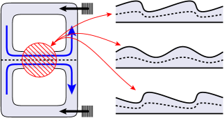
The type of device studied in the present paper differs in several aspects from a drift ratchet. It does not require an oscillating flow, which is difficult to generate and maintain experimentally [20, 21, 22], but operates with a stationary flow field. The flow is confined to a channel with variable width – as for a drift ratchet – but with ends connected to each other in some way, leading e.g. to a ring-like or “figure eight” geometry, cf. Fig 1. Spherical particles will then accumulate in particular regions of the channel. In a previous experimental work the figure eight geometry was realized to separate particles immersed in a fluid by means of electric fields [29, 30]. In this experiment, a steady flow of the fluid was maintained by surface acoustic waves leading to acoustic streaming [15].

For the sake of simplicity we restrict our analysis to two spatial dimensions. The relevant mechanisms put forward in this work leading to an accumulation do not depend on the two-dimensional character and will work as well in three dimensions. In the experimental realization [29, 30] the flow channels are bounded by a rigid substrate only at the bottom, the remaining boundary is a free interface between water and air. A reduction of this very situation to two dimensions is not obvious. To still include the effects of different types of boundaries in the two-dimensional model we consider two cases, one with two no-slip boundaries corresponding to two impenetrable walls confining the fluid and the other one with a no-slip and a perfect slip boundary. The latter boundary mimics a free boundary with dominant surface tension such that the flow only leads to a negligible deformation of the equilibrium shape.

Figure 1: (Color online) Sketch of the channel geometry. The middle part contains an asymmetric channel, which is doubly closed by two loops. The dashed line indicates the streamline connecting the stagnation points of the flow and separating the two flow chambers. The geometry may represent either closed channels or a wetting pattern on a flat substrate. The flow driving is exemplified to be acoustically driven as indicated by the two blocks of parallel lines representing surface-acoustic waves which propagate in the directions of the arrows [29, 30].

The paper is organized as follows. In Section 2 we introduce the flow field which is then used for transporting particles. In Section 3 we analyze the hydrodynamic and random forces on the particles and formulate the long-time particle accumulation pattern in terms of a stationary Fokker–Planck equation. Section 4 makes a distinction between possible accumulations caused by a volume and a boundary effect. In pressure-driven channel flows only the latter may occur, which is then investigated numerically in Section 5.

2 The flow fields

We consider stationary incompressible flows in the limit of vanishing Reynolds numbers. The velocity $\mathbf{v}(\mathbf{x})$ and pressure $p(\mathbf{x})$ fields are solutions of the stationary Stokes equations,

$$\mathbf{0}=-\boldsymbol{\nabla}p(\mathbf{x})+\eta\Delta\mathbf{v}(\mathbf{x})+\mathbf{f}(\mathbf{x}),$$ (1)

$$0=\operatorname{div}\mathbf{v}(\mathbf{x}),$$ (2)

where $\eta$ denotes the viscosity of the fluid and $\mathbf{f}$ is a conservative externally applied body force which gives rise to the flow fields $p(\mathbf{x})$ and $\mathbf{v}(\mathbf{x})$. The velocity field is subject to the kinematic boundary condition, i. e. for immobile boundaries,

$$\mathbf{v}\!\boldsymbol{\cdot}\!\mathbf{N}=0,$$ (3)

representing the fact that all boundaries of the fluid domain $\partial\Omega$ are material lines of the flow. $\mathbf{N}$ denotes the normal vector. At immobile sticky walls, also the velocity components parallel to the tangent vectors $\mathbf{T}^{(\alpha)}$ vanish,

$$\mathbf{v}\!\boldsymbol{\cdot}\!\mathbf{T}^{(\alpha)}=0\quad\text{for all $\alpha$.}$$ (4)

For a free boundary, such as the interface between water and air, the tangential velocity at the boundary is determined by the mechanical stress balance. For the velocity field, this reduces to the perfect slip condition

$$T_{i}^{(\alpha)}\left(\frac{\partial v_{i}}{\partial x_{j}}+\frac{\partial v_{j}}{\partial x_{i}}\right)N_{j}=0\quad\text{for all $\alpha$.}$$ (5)

In general, at a free boundary the shape of the interface between two fluids depends itself on, and reacts back to, the flow and pressure fields in the fluid. Here we restrict ourselves to flows in a given domain on the boundaries of which the kinematic boundary condition (3) and either the no-slip (4) or the perfect slip condition (5) hold. The full description of free fluid surfaces with surface tension can be found in references [31, 32]. In the numerical examples in Sec. 5 below, we will find that the type of the boundary condition has strong influence on the particle accumulation taking place near the boundary.

3 Hydrodynamic particle transport

The flow fields solving the Stokes equations (1) and (2) in combination with the boundary conditions (3) and (4) or (5) are used to advect small spherical particles. If such a particle is a point-particle at position $\mathbf{X}(t)$, it cannot be distinguished from the fluid material at this point. It is therefore transported with the velocity of the fluid itself, $\dot{\mathbf{X}}(t)=\mathbf{v}(\mathbf{X}(t))$.

The motion of an extended spherical particle with small but non-vanishing radius $R$ about $\mathbf{X}(t)$, however, is qualitatively different from that of a point-particle. The force on such a particle is the integral of the fluidic stress over the particle’s oriented surface, denoted by $\mathbf{F}_{\mathbf{v}}(t)$ and $\mathbf{F}_{p}(t)$ for the viscous and the pressure contributions of the stress, respectively. An additional random force $\mathbf{F}_{\boldsymbol{\xi}}(t)$ takes thermal fluctuations into account. For a small particle of mass $m$, the inertial force is negligible [33], resulting in an overdamped motion, described by the Langevin equation

$$0=m\ddot{\mathbf{X}}(t)=\mathbf{F}_{\mathbf{v}}(t)+\mathbf{F}_{p}(t)+\mathbf{F}_{\boldsymbol{\xi}}(t).$$ (6)

The pressure contribution $\mathbf{F}_{p}(t)$ is obtained by expanding the pressure field in a Taylor series around the particle center $\mathbf{X}$ and integrating over the particle surface $S_{R}(\mathbf{X})$,

$$\mathbf{F}_{p}=-\oint\limits_{\makebox[7.00002pt]{\hss$\scriptstyle S_{R}(\mathbf{X})$\hss}}p\mathbf{N}\,dA=-\frac{4\pi}{3}R^{3}\boldsymbol{\nabla}p(\mathbf{X})-\mathcal{O}(R^{5}).$$ (7)

The viscous contribution $\mathbf{F}_{\mathbf{v}}(t)$ cannot be readily obtained, since the particle alters the velocity field: It poses a spherical no-slip boundary to the surrounding fluid. In the Stokes regime, in which the acceleration field of the fluid caused by the movement of the particle can be neglected, we may employ Faxén’s theorem of translational motion to describe this effect [34, 32]. The force $\mathbf{F}_{\mathbf{v}}(t)$ is then given in terms of a modified velocity field $\tilde{\mathbf{v}}$, which is evaluated at the center of the particle,

$$\mathbf{F}_{\mathbf{v}}=6\pi\eta R\bigl{[}-\dot{\mathbf{X}}+\tilde{\mathbf{v}}(\mathbf{X})+\Delta\tilde{\mathbf{v}}(\mathbf{X})\,R^{2}/6\bigr{]}.$$ (8)

In contrast to the true velocity field $\mathbf{v}$ which describes the flow in the presence of the particle, the auxiliary field $\tilde{\mathbf{v}}$ is also defined within the region which is covered by the particle. Still, it contains all perturbations caused by the particle, cf. Appendix A for the definition and Ref. [32] for a detailed discussion. Unfortunately, determining $\tilde{\mathbf{v}}$ is as elaborate as solving the full stationary problem in the presence of the particle. In the next section we can, however, make use of the fact that $\tilde{\mathbf{v}}$ is a solenoidal vector field.

The third contribution to the force on a particle in Eq. (6), i.e. the fluctuating force $\mathbf{F}_{\boldsymbol{\xi}}$, reads at thermodynamic equilibrium [35, 36, 37],

$$\mathbf{F}_{\boldsymbol{\xi}}(t)=\sqrt{2d\,}\,{\boldsymbol{\xi}}(t),$$ (9)

with the noise strength $d=6\pi\eta R\,k_{\text{B}}T$, and ${\boldsymbol{\xi}}(t)$ being Gaussian white noise,

$$\bigl{\langle}\xi_{i}(t)\bigr{\rangle}=0,$$ (10)

$$\bigl{\langle}\xi_{i}(t)\xi_{j}(s)\bigr{\rangle}=\delta_{ij}\,\delta(t-s).$$ (11)

We neglect deviations from the equilibrium expression of the fluctuation–dissipation theorem, which become relevant for large velocity gradients only, see Refs. [38, 39], and references therein. Further, we assume a dilute solution of particles such that hydrodynamic particle–particle interactions can be ignored in the Langevin equation (6). The overdamped Langevin equation (6), solved for the particle velocity is then equivalent to a Fokker–Planck equation for the probability density $\rho(\mathbf{X},t)$ of the particle centers,

$$\partial_{t}\rho(\mathbf{x},t)=-\operatorname{div}\bigl{(}\rho(\mathbf{x})\,\mathbf{d}(\mathbf{x})\bigr{)}+D\Delta\rho(\mathbf{x}).$$ (12)

The diffusion constant is given by the Sutherland–Einstein relation

$$D=\frac{d}{(6\pi\eta R)^{2}}=\frac{k_{\text{B}}T}{6\pi\eta R},$$ (13)

and the drift velocity $\mathbf{d}$ reads, combining (7) and (8),

$$\mathbf{d}(\mathbf{x})=\tilde{\mathbf{v}}(\mathbf{x})+\frac{R^{2}}{6}\Delta\tilde{\mathbf{v}}(\mathbf{x})-\frac{2R^{2}}{9\eta}\boldsymbol{\nabla}p(\mathbf{x})+\mathcal{O}(R^{5}).$$ (14)

The remaining term $\mathcal{O}(R^{5})$ comes from the Taylor expansion in Eq. (7). The viscous terms containing the modified velocity field $\tilde{\mathbf{v}}$ are exact. In the present paper, we focus on the long-time limit of the particle distribution, which is governed by the condition $\partial_{t}\rho(\mathbf{x},t)=0$, leading to the stationary Fokker–Planck equation

$$0=-\operatorname{div}\bigl{(}\rho(\mathbf{x})\,\mathbf{d}(\mathbf{x})\bigr{)}+D\Delta\rho(\mathbf{x}).$$ (15)

4 Volume- versus boundary-accumulation

As an accumulation of particles we refer to an inhomogeneous distribution of particles $\rho(\mathbf{x})$. First, we note that the uniform distribution $\rho(\mathbf{X})=\textit{const}$ is a possible solution of the stationary Fokker–Planck equation (15) in case of a solenoidal drift field, $\operatorname{div}(\mathbf{d})=0$ [12, 18]. Whether this solution is the physically realized one, depends only on the boundary conditions. Deviations from a uniform stationary particle density are caused either by particular boundary conditions which impose a non-vanishing gradient of the particle density at the boundary, or a non-vanishing divergence of the vector field $\mathbf{d}(\mathbf{x})$. We refer to the former and the latter case as boundary effect and volume effect, respectively.

4.1 Volume effect

The volume accumulation mechanism takes place for a drift velocity having a non-vanishing divergence, $\operatorname{div}(\mathbf{d})\neq 0$. The homogeneous distribution $\rho(\mathbf{X})=\textit{const}$ then is not a solution of equation (15), irrespectively of any boundary condition. Whether the drift field is solenoidal, depends on the shape of the particle. A particle of complicated shape generally gives rise to a drift field with non-vanishing divergence. Examples can be found in the literature [40, 41, 42, 43, 44, 18].

In the special case of a spherical particle, however, the drift velocity $\mathbf{d}(\mathbf{X})$ is given by equation (14). Although the velocity field $\tilde{\mathbf{v}}(\mathbf{X})$ is not known explicitly, it is known to be divergence-free. The same is true for its Laplacian. Only the pressure gradient may lead to a non-vanishing divergence of $\mathbf{d}(\mathbf{x})$. Taking the divergence of Eq. (14) one obtains in leading order the Laplacian of the pressure $p$, which can be determined by the Stokes equation (1) to yield

$$\operatorname{div}(\mathbf{d})=\frac{2R^{2}}{9\eta}\Delta p=\frac{2R^{2}}{9\eta}\operatorname{div}(\mathbf{f}).$$ (16)

In a long modulated channel, where the flow is driven either by a pressure difference, by a constant force, or by an inflow velocity profile, the drift velocity $\mathbf{d}(\mathbf{x})$ is indeed solenoidal. For these situations we state that all volume effects vanish exactly, and inhomogeneities in the particle density can only be caused by the boundaries.

4.2 Boundary effect

The boundary condition for the particle density in the fluid is given by the condition of vanishing normal particle flux,

$$0=\mathbf{N}\!\boldsymbol{\cdot}\!(\rho\,\mathbf{d}-D\,\boldsymbol{\nabla}\rho),$$ (17)

which guarantees that particles cannot cross the boundary. In case of a vanishing normal drift velocity $\mathbf{N}\!\boldsymbol{\cdot}\!\mathbf{d}=0$ only the uniform distribution $\rho(\mathbf{x})=\textit{const}$ is allowed. Vice versa, an inhomogeneous particle distribution can only emerge, if the normal drift at the boundary does not to vanish.

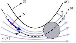
The velocity field $\tilde{\mathbf{v}}$, which is the leading-order term in the drift velocity (14), satisfies the kinematic boundary condition (3) at the boundary of the fluid domain. As it does not provide a normal component, one might expect that neither a volume effect nor a boundary accumulation is achieved from the leading-order term in Eq. (14). A close look on a spherical particle in the vicinity of a boundary, however, reveals that there is indeed such a normal component. Relevant in Faxén’s theorem (8) is the modified velocity field $\tilde{\mathbf{v}}$ at the center of the particle, which cannot touch the physical boundary but stays at least one radius apart from it. The no-flux boundary condition (17) must therefore be imposed on an effective boundary $\partial\Omega^{\prime}$ which has constant distance $R$ from the physical boundary $\partial\Omega$ of the fluid. Both are sketched in Fig. 2. Neither the streamlines of the flow nor the field-lines of the particle drift velocity need to have a constant distance from the boundary. Instead, some of the field-lines cross the boundary $\partial\Omega^{\prime}$ of the region which is accessible to the particle centers. In Fig. 2 one of these crossing points is marked. There, the normal component of $\mathbf{d}(\mathbf{X})$ is positive, i. e. pointing to the boundary whence leading to a deposition of particles at the boundary. Accordingly, a negative normal component results in a depletion zone. Both effects will be found in the numerical simulations below, see Fig. 5.

Figure 2: (Color online) The boundaries of the fluid domain $\Omega$ and of the accessible region $\Omega^{\prime}$ for the particle center. Their distance equals the particle radius $R$ everywhere. At the boundary $\partial\Omega^{\prime}$ the normal component of the drift velocity, and thus also of the drag force, are not zero. This is exemplified at the point marked by a cross.

The given argument in the foregoing paragraph is a geometrical explanation for the leading-order terms of the hydrodynamic interaction between particle and wall. A general theory of hydrodynamic interactions in asymmetric geometries is presently not available. A known effect of the hydrodynamic interaction is a decrease of the fluid velocity induced by the presence of the particle. Additionally, one obtains the Saffman lift force [45] which drives the particle away from the boundary. The magnitude of this force is proportional to the squared particle radius and to the mismatch between the true particle velocity and the unperturbed fluid velocity. Reference [46] provides explicit expressions for the correction terms from hydrodynamic interaction between particle and boundary. The force densities given there comprise a component, diverging at the effective boundary $\partial\Omega^{\prime}$, corresponding to the hard-core interaction. The next leading-order term in the particle radius $R$ is the random force, being proportional to $R^{1/2}$. The tangential force leading to the slowing down of the particle is proportional to $R$, and the Saffman lift force scale as $R^{2}$.

About the normal projection of the second-order terms in the drift velocity $\mathbf{d}(\mathbf{x})$, being proportional to $R^{2}$ in Eq. (14), we cannot say much. Generally, they may give rise to a boundary effect. The magnitude of this effect, however, scales quadratically with the particle radius $R$ and is therefore expected to be smaller than the hard-sphere boundary effect. Furthermore, for pressure-driven flows in long channels, the pressure gradient at the boundary is oriented along the channel rather than normal to it.

5 Numerical examples in modulated channels

The aim of this paper is to provide a qualitative picture of the influence of the domain shape on the particle density. In order to achieve this goal we have to restrict the following numerical analysis to the leading-order terms of the forces. These are the geometrical interaction between particles and wall, as depicted in Fig. 2, and the random forces. By omitting terms which are quadratic in the particle radius, we may also replace the unknown velocity field $\tilde{\mathbf{v}}$ by the unperturbed velocity $\mathbf{v}$.

Using these simplifications, the full interaction between particle and wall is replaced by a hard-core interaction preventing the particle from penetrating the wall. We are aware that this approximation may be quite crude for the quantitative description of a real particle in a real fluid. However, the analysis above shows that the only terms which lead to an accumulation are the normal forces on the particles in the vicinity of the boundary. In the hard-core model, this happens instantaneously as the particle touches the wall. The force is localized on the effective boundary $\partial\Omega^{\prime}$. Corrections to the force, as detailed in Ref. [46] smear out the force such that the particle is slowed down already in the vicinity of the wall. This will not alter the qualitative picture obtained here by the hard-core interaction. Whether this approximation is really justifiable, can be decided only by extensive numerical calculations of the hydrodynamic interactions, a task which is beyond the scope of the present study.

Next, we solve the Fokker–Planck equation

$$0=-\mathbf{v}\!\boldsymbol{\cdot}\!\boldsymbol{\nabla}\rho+D\Delta\rho\quad\text{in $\Omega^{\prime}$,}$$ (18)

with the boundary condition

$$0=\mathbf{N}^{\prime}\!\boldsymbol{\cdot}\!(\rho\,\mathbf{v}-D\boldsymbol{\nabla}\rho)\quad\text{on $\partial\Omega^{\prime}$.}$$ (19)

The vector $\mathbf{N}^{\prime}$ denotes the normal vector of the effective boundary $\partial\Omega^{\prime}$. The velocity field $\mathbf{v}$ is taken from the numerical solution of the Stokes equations in $\Omega$ with the boundary conditions from Sec. 2, the domain $\Omega$ being a periodic two-dimensional channel of modulated width. Its two boundaries have different geometries, one is straight, while the other is curved, see Fig. 4. We choose the shape of the curved boundary to be given by the periodic function $g$, which is implicitly defined by the relation

$$g(z)=\sin\bigl{(}2\pi z-a\,g(z)\bigr{)}.$$ (20)

Figure 3: (Color online) A detail of the computational mesh near the boundary. The outermost layer of finite elements represents the zone which cannot be entered by the particle centers. The element sides of this layer constitute the two boundaries $\partial\Omega$ and $\partial\Omega^{\prime}$, compare with Fig. 2.

Figure 4: (Color online) Example-flows in periodically continued two-dimensional channels, modulated according to Eq. (20) with asymmetry parameter $a=0.8$. In panel (a) both boundary conditions are no-slip, while in (b) the straight boundary carries a perfect-slip condition. The flow direction is from left to right, driven by a pressure difference of $\Delta p=1\,\nobreak\mbox{Pa}$ per length $L=10^{-4}\nobreak\mbox{m}$ of the unit cell. The viscosity is that of water. The black lines represent streamlines.

Figure 5: (Color online) Example-densities of particle centers in the flows of Fig. 4, normalized to an average value of unity. The densities have been calculated as the solution of the Fokker–Planck equation (15) with $\Delta p/T=3.3\times 10^{-6}\,\nobreak\mbox{Pa}/\nobreak\mbox{K}$ which corresponds to a Péclet number of $\textit{Pe}\approx 16$. At the boundaries, the black zone with zero density indicates the area which the particle centers cannot enter. It is one particle radius wide, here $R=10^{-2}L$. The thin black lines indicate level lines of the density.

The number $a$ parametrizes the asymmetry of the shape, yielding a sinusoidal shape for $a=0$, while shapes with $a\neq 0$ have alternating steep and flat flanks. For $a>0$ the flat flanks have positive and the steep flanks have negative inclination, and vice versa for $a<0$. The values $g(z)$ can be evaluated iteratively, starting with $\sin(2\pi z)$.

The parameter regime of equation (18) is characterized by the dimensionless Péclet number, which expresses the ratio of advective to diffusive transport. We here define the global Péclet number as

$$\textit{Pe}=\frac{\bar{x}\bar{v}}{D}=\frac{3\pi L^{2}}{128\,k_{\text{B}}}\>R\>\frac{\Delta p}{T}.$$ (21)

For the stationary particle distribution, there is no difference between a weakly driven system and one at a high temperature, as long as the ratio $\Delta p/T$ is the same. In the numerical calculations for several different temperatures, we therefore used the same numerically obtained velocity field, driven by a unit pressure difference $\Delta p=1\,\nobreak\mbox{Pa}$ along the channel length $L=10^{-4}\,\nobreak\mbox{m}$.

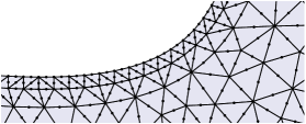
The computational mesh for the numerical solutions has to provide both boundaries, $\partial\Omega$ and $\partial\Omega^{\prime}$. Figure 3 shows a detail of the employed mesh near a boundary. The outermost layer of finite elements build the zone of constant width $R$ which cannot be entered by the particle centers. This zone can be identified in Fig. 5 as the zone near the boundary, showing a vanishing particle density.

5.1 Longitudinal accumulation

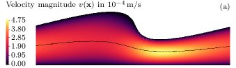
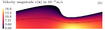
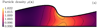
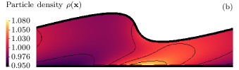
Figure 4 presents two velocity fields in the unit cell of a channel with asymmetry parameter $a=0.8$. They differ by the boundary condition at the straight wall: Panel (a) presents no-slip and (b) perfect slip boundary conditions. The corresponding solutions of the stationary Fokker–Planck equation (18) with boundary condition (19) are illustrated in Fig. 5. The qualitative form of the stationary distributions is quite intuitive. Left of the bottleneck we find an accumulation zone of the particles. Resulting from the main flow direction from left to right, the particles are concentrated at the left side, just upstream in front of the bottleneck. This result can be understood by means of Fig. 2. Left and right of the bottleneck we find regions where streamlines cross the effective boundary $\partial\Omega^{\prime}$, leading to a non-vanishing drift component in normal direction. This normal component results in the accumulation that we see in Fig. 5 for $\textit{Pe}\approx 16$. This corresponds to a slightly advection-dominated transport of particles. For smaller Péclet numbers, the diffusion becomes more dominant, resulting in a smoother particle distribution than in Fig. 5. For larger Péclet numbers, the maxima of the distribution near the boundaries become more pronounced.

5.2 Influence of the boundary conditions

Comparing the particle densities in Fig. 5 for different boundary conditions of the velocity field, one finds the extremal values to be more pronounced in the case with a perfect-slip condition. The reason for this difference is that the slip condition allows a larger velocity at the boundary, giving rise also to a larger normal component, which then causes the accumulation effect. We expect that in general free surfaces, providing perfect slip boundary conditions, cause larger accumulation effects than sticky walls, as long as the particles do not leave the fluid nor cause major deformations of the free surface.

5.3 Perpendicular accumulation and sorting

The two accumulation patterns in Fig. 5 do not only differ with respect to their magnitude. So far, we have only looked at the inhomogeneity along the channel orientation, by stating that there are concentration and depletion zones in front of the bottleneck and behind, respectively. For a small channel as in experimental applications also the distance of the accumulation centers will be prohibitively small. A performance characteristic of much more interest is the accumulation perpendicular to the channel orientation. This may be achieved by a branching channel where the flow is split along the streamline that ends in a stagnation point. Such a structure has been experimentally realized as a eight-shaped geometry and used for separating particles with external electric forces [29]. Particles immersed in this flow do not generally follow the streamlines and thus can cross the separating streamline and pass from one basin into the other. This leads to a relative accumulation of particles in one of the basins, if they were originally equally distributed.

The quality of separation is characterized by the amounts of particles that are above and below the separating streamline indicated in Fig. 4. For this purpose we separately integrate the particle density in the two regions $\Omega^{\prime}_{+}$ and $\Omega^{\prime}_{-}$, representing the accessible regions above ($+$) and below ($-$) the separating streamline, respectively. The resulting two probabilities per area $P_{+}/\bigl{|}\Omega^{\prime}_{+}\bigr{|}$ and $P_{-}/\bigl{|}\Omega^{\prime}_{-}\bigr{|}$ of finding a particle above or below the streamline can be used to provide a measure for the relative accumulation of particles in one of the basins. We use the quantity

$$r:=\frac{P_{+}}{\bigl{|}\Omega^{\prime}_{+}\bigr{|}}\biggm{/}\frac{P_{-}}{\bigl{|}\Omega^{\prime}_{-}\bigr{|}}$$ (22)

as a measure for the relative accumulation in the upper basin, which is the one with the curved boundary. The denominators $\bigl{|}\Omega^{\prime}_{+}\bigr{|}$ and $\bigl{|}\Omega^{\prime}_{-}\bigr{|}$ represent the volumes of the regions above and below the separating streamline, respectively.

Figure 6: (Color online) The relative accumulation $r$ perpendicular to the main flow direction for flows with no-slip boundary conditions. Values smaller than unity correspond to an accumulation of particles below the separating streamline, near the straight wall. In panel (a) the temperature is varied for a fixed particle radius $R=10^{-2}L$. In panels (b) and (c) the particle radius is varied for two selected temperatures, $\Delta p/T=3.3\times 10^{-7}$ and $3.3\times 10^{-8}$, respectively.

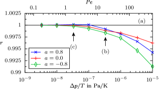
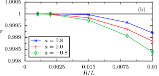
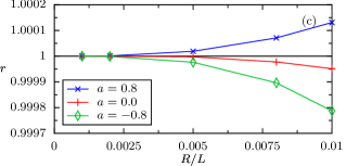
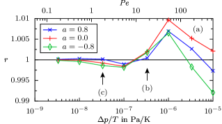
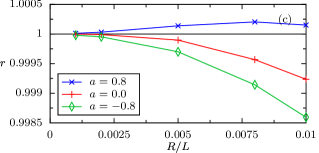
Figure 6 displays the resulting relative accumulation for flows with two no-slip boundaries in three different channel geometries, indicated by different values of the asymmetry parameter $a$. The upper panel shows the ratio $r$ as a function of the inverse temperature. The first observation is that the effect vanishes for vanishing driving – or equivalently, for infinite temperature. For the majority of the parameter values the result is smaller than unity. This corresponds to an accumulation of particles at the side of the straight wall. This appears as a general tendency, which was found also for other shapes. The relative accumulation effect is at most one percent for the smallest temperature that was used in the calculation. As expected, it vanishes for very small driving strengths $\Delta p/T$. In order to demonstrate that this small effect is not an artifact of the numerical calculation, also the flows in the mirrored channels with inverted pressure differences were considered. For symmetry reasons both configurations yield identical accumulation ratios. The numerical differences between these are found to be smaller than the line thickness in Fig. 6. For two temperature values, also the particle radius was varied. Panels (b) and (c) of Fig. 6 depict the ratio $r$ as a function of the radius. Again, the effect vanishes with vanishing radius. This is the expected behavior, because a point-particle can come arbitrarily close to the physical boundary.

An interesting aspect of the accumulation results in Fig. 6 is the fact that the channel with $a=0.8$ behaves differently from the one with $a=-0.8$. We find as a general tendency that the channel which suddenly widens and slowly narrows ($a=-0.8$) in flow direction yields better accumulations than the suddenly narrowing one. The channel with the sinusoidal shape ($a=0$) yields accumulation results somewhere in between.

5.4 Accumulation inversion

Another remarkable property of the accumulation mechanism can be observed for the flow in the channel with asymmetry parameter $a=0.8$. Here, we find values of $r$ also being larger than unity. Particles in this parameter regime are transported towards the curved boundary rather than towards the straight one. The occurrence of both values corresponds to an inversion of the transport direction. Panel 6c confirms that the values larger than unity, which we found in 6a, persist also for several smaller radii. Note that for each radius, a different numerical mesh was used in order to represent the correct boundary $\partial\Omega^{\prime}$. The inversion found here is not readily usable for sorting particles because it takes place upon varying the parameter $\Delta p/T$ and not the radius $R$. Moreover, the effect seems far too small to be of experimental relevance. Still, the occurrence of accumulation inversion is an interesting effect.

Figure 7: (Color online) The same as Fig. 6 for a flow with perfect-slip boundary condition at the straight wall.

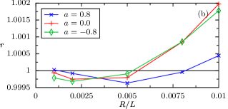
Employing a perfect-slip boundary condition at the straight wall leads to a qualitatively different parameter dependence of the accumulation. Fig. 7 depicts the relative accumulation for the same driving parameters as Fig. 6. Again, the accumulation vanishes for vanishing driving and for vanishing particle radius. The direction of the accumulation depends now much stronger on the driving strength $\Delta p/T$. As a qualitative picture, we here observe a particle of a given size to be pushed towards the curved or towards the straight wall, depending on the pressure difference. This accumulation inversion can also be found in Fig. 7b as a function of the particle radius. Thus, we may find particles with different radii accumulated in the two different parts of the channel. For small particles this effect though is small.

6 Conclusions

We analyzed the accumulation of small spherical particles in two-dimensional fluid flows confined to channels with one curved boundary. It turned out that accumulation due to volume effects is impossible if the flow is driven by a pressure difference or a homogeneous force. In this case, only boundary accumulation effects are possible. For that to happen the normal projection of the particle drift at the boundary must not vanish. Otherwise, only the trivial uniform distribution of particles is achieved. In order to simplify the numerical calculations we employed a hard-core interaction model for the intricate interaction between a particle and a wall. Both imply non-vanishing normal components of the drift velocity near the boundary, thus giving rise to a small accumulation effect, which scales with the particle radius.

We compared no-slip and perfect-slip boundary conditions for the velocity fields in the channels. The latter is a simplification of the free-surface boundary condition which is realized in some experiments. We observed that the type of the boundary condition on the flow has severe implications on the resulting accumulation pattern of immersed particles. Free surfaces generally caused larger accumulation effects showing also qualitatively different and interesting properties, such as an inversion of the accumulation direction, depending on the radius of the considered particle. This inversion might be put to beneficial use for a separation of particles of varying size.

Acknowledgments. We thank Dr. Uwe Thiele for valuable comments on the manuscript. Financial support is gratefully acknowledged from the Deutsche Forschungsgemeinschaft (DFG) via Sonderforschungsbereich 486, Projekt B13, the DFG grants HA 1517/25-2 and HA 1517/29-1, and also by the German Excellence Initiative via the Nanosystems Initiative Munich (NIM).

Appendix A Velocity fields

The following three velocity fields are relevant in Faxén’s theorem to express the motion of a spherical particle in an external velocity field: First, in absence of the particle, there is the unperturbed velocity field solving the Stokes equations (1) and (2). The flow field satisfies the integro-differential equation [34],

$$v_{k}(\mathbf{y})=\oint\limits_{\partial\Omega}dA(\mathbf{x})\,N_{j}(\mathbf{x})\bigl{[}{\mathcal{K}}_{ik}(\mathbf{x}-\mathbf{y})\,\sigma_{ij}(\mathbf{x})-{\mathcal{T}}_{ijk}(\mathbf{x}-\mathbf{y})\,v_{i}(\mathbf{x})\bigr{]},$$ (23)

where the external conservative force is taken into account by defining a modified pressure containing the potential of the force. The kernels ${\mathcal{K}}$ and ${\mathcal{T}}$ may be chosen to be the Green functions for the unbounded Stokes problem,

$${\mathcal{K}}_{ik}(\mathbf{r}) =\frac{1}{8\pi\eta}\Bigl{(}\frac{\delta_{ik}}{r}+\frac{r_{i}r_{k}}{r^{3}}\Bigr{)},$$ (24)

$${\mathcal{T}}_{ijk}(\mathbf{r}) =-\frac{3}{4\pi}\frac{r_{i}r_{j}r_{k}}{r^{5}}.$$ (25)

The transformation of the Stokes equations into an equation on the boundary only is essential for Faxén’s theorem. This implies that only conservative forces may drive the fluid.

The second flow field which is important is the true velocity field in presence of the particle. We denote it with $\bar{\bar{\mathbf{v}}}$. It satisfies a similar relation as (23), but the particle cuts a spherical region out of the domain $\Omega$. The boundary integral is then carried out also over the surface of the particle,

$$\bar{\bar{v}}_{k}(\mathbf{y})=\oint\limits_{\makebox[7.00002pt]{\hss$\scriptstyle\partial\Omega\cup S_{R}(\mathbf{X})$\hss}}dA(\mathbf{x})\,N_{j}(\mathbf{x})\bigl{[}{\mathcal{K}}_{ik}(\mathbf{x}-\mathbf{y})\,\bar{\bar{\sigma}}_{ij}(\mathbf{x})-{\mathcal{T}}_{ijk}(\mathbf{x}-\mathbf{y})\,\bar{\bar{v}}_{i}(\mathbf{x})\bigr{]}.$$ (26)

The third relevant velocity field is the one that is used in Faxén’s theorem. It must be evaluated at the center of the sphere. This effective velocity field $\tilde{\mathbf{v}}$ is obtained by carrying out the integral in (26) over the particle surface explicitly as

$$\tilde{v}_{k}(\mathbf{y}):=\oint\limits_{\partial\Omega}dA(\mathbf{x})\,N_{j}(\mathbf{x})\bigl{[}{\mathcal{K}}_{ik}(\mathbf{x}-\mathbf{y})\,\bar{\bar{\sigma}}_{ij}(\mathbf{x})-{\mathcal{T}}_{ijk}(\mathbf{x}-\mathbf{y})\,\bar{\bar{v}}_{i}(\mathbf{x})\bigr{]}.$$ (27)

For the details of this calculation see Ref. [32]. This effective velocity field is is then defined in the whole domain $\Omega$ and can be evaluated at the center of the particle. It is used for expressing the force on a particle in Eq. (8). Note that the boundary values of the true velocity field $\bar{\bar{\mathbf{v}}}$ enter the definition of $\tilde{\mathbf{v}}$. As a solution of the Stokes equation with appropriate pressure field, it is solenoidal. We make use of this property in Sec. 4.1.

References

- [1] H. A. Stone, A. D. Stroock, and A. Ajdari, Annu. Rev. Fluid Mech. 36 (2004) 381.
- [2] D. Figeys and D. Pinto, Anal. Chem. 72 (2000) 330A.
- [3] J. C. T. Eijkel and A. van den Berg, Electrophoresis 27 (2006) 677.
- [4] C. Marquet, A. Buguin, L. Talini, and P. Silberzan, Phys. Rev. Lett. 88 (2002) 168301.
- [5] R. Eichhorn, P. Reimann, and P. Hänggi, Phys. Rev. Lett. 88 (2002) 190601.
- [6] R. Eichhorn, P. Reimann, and P. Hänggi, Phys. Rev. E 66 (2002) 066132.
- [7] L. R. Huang, E. C. Cox, R. H. Austin, and J. C. Sturm, Science 304 (2004) 987.
- [8] M. Yamada, M. Nakashima, and M. Seki, Anal. Chem. 76 (2004) 5465.
- [9] A. Ros, R. Eichhorn, J. Regtmeier, T. T. Duong, P. Reimann, and D. Anselmetti, Nature 436 (2005) 928.
- [10] A. Ajdari, Phys. Rev. E 61 (2000) R45.
- [11] L. Gorre-Talini, S. Jeanjean, and P. Silberzan, Phys. Rev. E 56 (1997) 2025.
- [12] Z. G. Li and G. Drazer, Phys. Rev. Lett. 98 (2007) 050602.
- [13] A. D. Strook, R. F. Ismagilov, H. A. Stone, and G. M. Whitesides, Langmuir 19 (2003) 4358.
- [14] D. V. Lyubimov, A. V. Straube, T. P. Lyubimova, Phys. Fluids 17 (2005) 063302.
- [15] A. Wixforth, C. Strobl, C. Gauer, A. Toegl, J. Scriba, and Z. Guttenberg, Anal. Bioanal. Chem. 379 (2004) 982.
- [16] Z. Guttenberg, A. Rathgeber, S. Keller, J. O. Rädler, A. Wixforth, M. Kostur, M. Schindler, and P. Talkner, Phys. Rev. E 70 (2004) 056311.
- [17] J. Lighthill, J. Sound Vib. 61 (1978) 391.
- [18] M. Kostur, M. Schindler, P. Talkner, and P. Hänggi, Phys. Rev. Lett. 96 (2006) 014502.
- [19] C. Kettner, P. Reimann, P. Hänggi, and F. Müller, Phys. Rev. E 61 (2000) 312.
- [20] S. Matthias and F. Müller, Nature 424 (2003) 53.
- [21] F. Müller, A. Birner, J. Schilling, U. Gösele, C. Kettner, and P. Hänggi, phys. stat. sol. (a) 182 (2000) 585.
- [22] S. Matthias, Experimenteller Nachweis einer Drift-Ratsche, Diplomarbeit der Mathematisch-Naturwissenschaftlich-Technischen Fakultät, Martin-Luther-Universität Halle, 2002.
- [23] P. Hänggi and R. Bartussek, Lect. Notes Phys. 476 (1996) 294.
- [24] P. Reimann and P. Hänggi, Appl. Phys. A 75 (2002) 169.
- [25] P. Reimann, Phys. Rep. 361 (2002) 57.
- [26] R. D. Astumian and P. Hänggi, Physics Today 55, No. 11 (2002) 33.
- [27] F. Jülicher, A. Ajdari, and J. Prost, Rev. Mod. Phys. 69 (1997) 1269.
- [28] P. Hänggi, F. Marchesoni, and F. Nori, Ann. Physik (Berlin) 14 (2005) 51.
- [29] C. Strobl, T. Frommelt, Z. Guttenberg, and A. Wixforth (in preparation).
- [30] T. Frommelt, Mischen und Sortieren mit SAW-Fuidik in Simulation und Experiment, PhD Thesis, Mathematisch–Naturwissenschaftliche Fakultät, Universität Augsburg, 2007.
- [31] M. Schindler, P. Talkner, and P. Hänggi, Phys. Fluids 18 (2006) 103303.
- [32] M. Schindler, Free–Surface Microflows and Particle Transport, PhD Thesis, Mathematisch–Naturwissenschaftliche Fakultät, Universität Augsburg, 2006.
- [33] E. M. Purcell, Am. J. Phys. 45 (1977) 3.
- [34] C. Pozrikidis, Boundary Integral and Singularity Methods for Linearized Viscous Flow, Cambridge University Press, Cambridge, 1992.
- [35] W. Sutherland, Philos. Mag. 9 (1905) 781; Phil. Mag. 3 (1902) 161.
- [36] A. Einstein, Ann. Phys. 17 (1905) 549.
- [37] M. von Smoluchowski, Ann. Phys. 21 (1906) 756.
- [38] J. M. Rubí and D. Bedeaux, J. Stat. Phys. 53 (1988) 125.
- [39] K. Miyazaki and D. Bedeaux, Physica A 217 (1995) 53.
- [40] P. G. de Gennes, Europhys. Lett. 46 (1999) 827.
- [41] M. Doi and M. Makino, Phys. Fluids 17 (2005) 103605.
- [42] M. Doi and M. Makino, Phys. Fluids 17 (2005) 043601.
- [43] M. Doi and S. F. Edwards, The theory of Polymer dynamics, Oxford University Press, Oxford, 1986.
- [44] S. Kim and S. J. Karilla, Microhydrodynamics: Principles and Selected Applications, Butterworth–Heinemann, Boston, 1991.
- [45] P. G. Saffman, J. Fluid Mech. 22 (1965) 385.
- [46] P. W. Longest, C. Kleinstreuer, and J. R. Buchanan, Computers & Fluids 33 (2004) 577.