Reduction of surface coverage of finite systems due to geometrical steps

Abstract

The coverage of vicinal, stepped surfaces with molecules is simulated with the help of a two-dimensional Ising model including local distortions and an Ehrlich-Schwoebel barrier term at the steps. An effective two-spin model is capable to describe the main properties of this distorted Ising model. It is employed to analyze the behavior of the system close to the critical points. Within a well-defined regime of bonding strengths and Ehrlich-Schwoebel barriers we find a reduction of coverage (magnetization) at low temperatures due to the presence of the surface step. This results in a second, low-temperature transition besides the standard Ising order-disorder transition. The additional transition is characterized by a divergence of the susceptibility as a finite-size effect. Due to the surface step the mean-field specific heat diverges with a power law.

I Introduction

The characterization of phase transitions becomes especially demanding in situations where the order parameter is not directly accessible by experiment. One example is the search for a nuclear liquid-gas phase transition. A considerable discussion can be found in the literature about the possibility to observe a negative heat capacity as one signal of such a possible liquid-gas phase transition Campi et al. (2005). Such negative heat capacities appear in finite systems which are adequately described within the microcanonical ensemble. We report here an observation that a transition with a divergent heat capacity can occur as a consequence of geometrical distortion rather than due to a phase transition even in a canonical treatment Fisher and Ferdinand (1967). This may shed some light on the nature of observed signals.

One meets a similar situation when describing the coverage of surfaces with molecules. There it is interesting to distinguish signals caused by phase transitions between different adsorbate arrangements from signals due to structural transitions at local deviations from the ideal surface geometry. Different surface defects have been studied within Ising models Chung et al. (2000) by density renormalization methods as well as Monte Carlo techniques. Non-universal features were observed and the critical exponent of the magnetization was found to be near 1/2 for infinite systems. A review on the vast literature about phase transitions in inhomogeneous systems can be found in Igloi et al. (1993).

We investigate here a finite-size two-dimensional Ising model suitable to simulate the coverage of surfaces by molecules. While the explicit simulation with realistic parameters was described in [Loppacher et al., 2006] we concentrate here on principal results how the surface modification is influencing the transitions and the critical exponents. We suggest that the occurrence of divergent (or negative) heat capacities is not a unique signal of a phase transition but can occur due to the geometrical distortion of the system accompanied by anomalous exponents, which even fulfills the scaling hypothesis.

The two-dimensional Ising model belongs to the most studied models. For an overview see [Kumar et al., 1983]. The exact solution Onsager (1944) shows a phase transition with a critical behavior:

spontaneous magnetization	$M$	$\sim$	$|T-T_{c}|^{\beta}$
magnetic field dependence	$H$	$\sim$	$|M_{T=T_{c}}|^{\delta}$
susceptibility	$\chi$	$\sim$	$|T-T_{c}|^{-\gamma}$
specific heat	$c_{H}$	$\sim$	$|T-T_{c}|^{-\alpha}$.

Two exponents are exactly known, i.e. $\beta=1/8$ [Yang, 1952] and $\gamma=1\frac{3}{4}$ [Abraham, 1973]. From asymptotic expansions and strong numerical evidence one has furthermore $\alpha=0$ and $\delta=15$ [Gaunt and Domb, 1970] where the specific heat diverges logarithmically. Weiss’ mean-field approximation instead leads to $\alpha=0$, $\beta=\frac{1}{2}$, $\gamma=1$, and $\delta=3$ [Jones and March, 1973]. Both sets of critical exponents fulfill the inequalities [Rushbrooke, 1963] $\alpha+2\beta+\gamma\geq 2$ and [Griffiths, 1965] $\alpha+\beta(1+\delta)\geq 2$ known as scaling hypothesis. These scalings are determining the corresponding universality classes with specific scaling functions for the magnetic field dependence of the magnetization Gaunt and Domb (1970); Kadanoff (1990). The universality of this phase transition in two dimensions has been experimentally confirmed Back et al. (1995). Recently, the universality has been investigated with respect to finite size scaling Rikvold et al. (1994) and oscillating fields Korniss et al. (2000).

Modifications of the scaling relation due to surface defects have been studied extensively, see citations in [Binder and Hohenberg, 1974]. Let us only mention some of the results found in print. The divergences of the specific heat for free and ferromagnetic boundaries in different Ising models have been studied for 40 years Fisher and Ferdinand (1967). The effect of a surface in an Ising model induces spatial correlations which could be treated with the help of a Ginzburg-Landau equation Mills (1971). The two-spin correlations induced by a line defect in an Ising square lattice are considered with the help of two-particle correlation functions McCoy and Perk (1980); Ko et al. (1985). Many-point correlation functions along a modified bond have been calculated as well Kadanoff (1981). The critical exponents for the magnetization of a line defect are known analytically Bariev (1979); Brown (1982); Bariev (2000).

We will present here a quadratic Ising model with a line defect and an additional change of the magnetic field along the line known as Ehrlich-Schwoebel barrier. This can mimic the surface coverage with molecules in the presence of an additional step. First we explain the model and present the numerical results. We will find that the Ehrlich-Schwoebel barrier induces an additional transition. Then in the third chapter we show that the commonly used standard mean-field model fails to explain the observations quantitatively. An effective model is suggested which accounts for the basic results. This effective model is then discussed in chapter IV with respect to the critical exponents and is compared to the mean-field exponents of the standard Ising phase transition.

II Ising model with surface step

In order to simulate the coverage of surfaces by molecules we imagine this surface as an $N\times N$ square lattice with a straight step across the middle of the lattice. The spin-up states describe a molecule sticking to the surface while the spin-down states describe the absence of a bound molecule. The interaction with the $j=4$ neighboring surface molecules is described by the coupling constant $J$. Across the surface step we choose a different coupling constant $J^{\prime}=J/\sqrt{2}$. The interaction of the surface molecules with the substrate background is modeled in analogy to the spin coupling with an external field. Therefore we shall use the external magnetic field as a synonym for the coupling of molecules with the background. At the sites adjacent to the step the magnetic field is augmented by an additional term, $H_{s}>0$. $H_{s}$ models the Ehrlich-Schwoebel barrier, which impedes the diffusion of adsorbates across surface steps. On top of the step edge $H_{s}$ is added to $H$, hence it locally reduces the attractive adsorbate-substrate interaction and mimics the lower density of coordination sites on top of the step edge. From below, $H_{s}$ is subtracted, thus it enhances the adsorbate-substrate interaction and models the higher number of coordination sites along the step. Motivated by the results of Ehrlich and Schwoebel on the stability of step arrays we chose the attractive and repulsive parts of the barrier equally high. Thus, the Ising Hamiltonian for the stepped square lattice reads:

$$-{\cal H}=\sum_{i,j}Js_{i}s_{j}+\sum_{i^{\prime},j^{\prime}}J^{\prime}s_{i^{\prime}}s_{j^{\prime}}+\sum_{i^{\prime},j}Js_{i^{\prime}}s_{j}$$

$$+\mu_{0}H\sum_{i}s_{i}+\mu_{0}\sum_{i^{\prime}}(H\pm H_{s})s_{i^{\prime}},$$ (1)

where $i$ sums over all $N(N-2)$ terrace sites, $i^{\prime}$ over the step sites, $j$ over all neighbors with coupling $J$ and $j^{\prime}$ over all neighbors with coupling $J^{\prime}$. Without fields $H$ and $H_{s}$ this Hamiltonian is an Ising square lattice with a ladder defect Igloi et al. (1993) and the exact critical exponent has been derived Bariev (1979) to be

$$\beta_{\rm H=0}={1\over 2\pi^{2}}{\rm arccos}^{2}\left(-{\rm tanh}{2(J-J^{\prime})\over k_{B}T}\right).$$ (2)

This shows that the critical exponent becomes dependent on the coupling strength and is therefore non-universal.

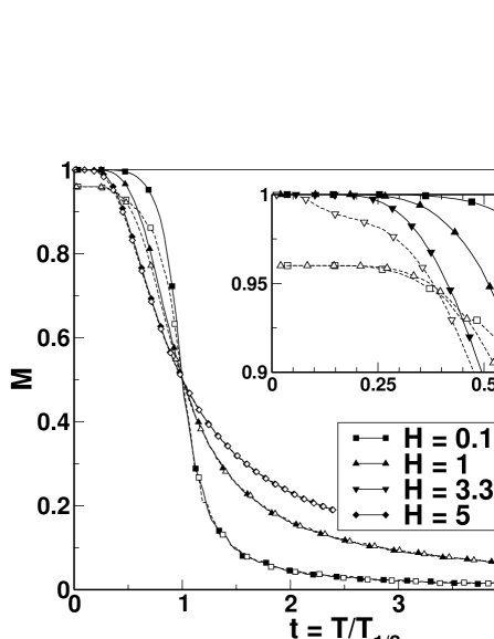
We solve the two-dimensional Ising model with the standard Metropolis scheme and the magnetization is now employed as measure for the surface coverage with molecules, plotted in Fig. 1. One sees that with increasing external field (or coupling of molecules to the background) a smearing of the standard Ising phase transition is obtained, which results in high temperature tails. This effect is well studied and experimentally confirmed Back et al. (1995). The ferromagnetic transition occurs only for vanishing magnetic fields. Fig. 1 also compares the solution of the two-dimensional Ising model with and without a surface step: For low values of the external magnetic field the step leads to a characteristic reduction of the magnetization at low temperatures.

Figure 1: Magnetization versus temperature scaled by the half-width temperature where the magnetization is $1/2$ for different external magnetic fields. The Ising lattice (50 $\times$ 50) with a step (open symbols and dashed lines) is compared with the one without a step (closed symbols and solid lines). The parameters are $J=1$, $J^{\prime}=1/\sqrt{2}$ and $\mu_{0}H_{s}=5$. Error bars are of or less than the size of the symbols.

III Construction of an effective mean-field model

III.1 Local mean-field model

This behavior can be understood by an effective two-spin model. We describe briefly in the following that the standard mean-field model, as e.g. used in the appendix of [Binder and Hohenberg, 1974], fails. For a lattice size of $N\times N$ spins and periodic boundary conditions, the system is homogeneous in the direction parallel to the step, thus we can restrict our considerations to the direction perpendicular to the step. We distinguish $N-2$ normal Ising spins and $1$ spin at each side of the step, for which the modified coupling constant $J^{\prime}$ and the Ehrlich-Schwoebel barrier term $H_{s}$ are taken into account Schinzer et al. (2000). All three kinds of spin experience an effective mean-field. We will denote the normal mean spin with $s$ and the mean spins at the step with $s^{\pm}$ according to the sign of the Ehrlich-Schwoebel barrier term, $\pm H_{s}$. $N-4$ of the sites occupied by normal spins see a mean-field $\tilde{H}$ consisting of the external field $H$ and the interaction with 4 neighbors, $4J$. The remaining two of the $N-2$ normal spins interact only with 3 normal spins and with one spin at the step. Therefore we have

$$\mu_{0}\tilde{H}=\mu_{0}H+{N-4\over N-2}4Js+{2\over N-2}(3Js+J{s^{+}+s^{-}\over 2}).$$ (3)

The spins along the step have two interactions with the same kind of spins, $2Js^{\pm}$, one neighbor with normal coupling, $Js$, a contribution from the coupling across the step, $J^{\prime}s^{\mp}$, and an interaction with the substrate of $H\pm H_{s}$. This results in

$$\mu_{0}\tilde{H}^{\pm}=\mu_{0}H\pm\mu_{0}H_{s}+2Js^{\pm}+J^{\prime}s^{\mp}+Js.$$ (4)

The partition function is then trivially written as

$$z = [2\cosh{(\beta\mu_{0}\tilde{H})}]^{(N-2)N}$$ (5)

$$\times[2\cosh{(\beta\mu_{0}\tilde{H}^{+})}]^{N}[2\cosh{(\beta\mu_{0}\tilde{H}^{-})}]^{N}$$

with the inverse temperature $\beta=1/k_{B}T$. The mean spins are calculated by expressions of the statistical averages, $s=\tanh{(\beta\mu_{0}\tilde{H})}$ and $s^{\pm}=\tanh{(\beta\mu_{0}\tilde{H}^{\pm})}.$ (3) and (4) represent the self-consistent mean-field equations for $s$ and $s^{\pm}$. This mean-field result is exactly equivalent to the Bragg-Williams method by minimizing the Gibbs functional and assuming that the many-spin correlation function factorizes into single-spin ones. Such mean-field equations for open surface defects have been investigated in [Mills, 1971; Binder and Hohenberg, 1974].

First it is instructive to solve this equation in the limit of zero temperature. Then one gets the values of the mean spins $\pm 1$ according to the sign of the mean fields (3) and (4). Consequently the total mean spin

$$M=\left(1-\frac{2}{N}\right)s+\frac{1}{N}(s^{+}+s^{-})$$ (6)

approaches the reduced value $M=1-{2\over N}$ for $T\to 0$ if $\tilde{H}>0\,\,{\rm and}\,\,(\tilde{H}^{+}\gtrless 0\,{\rm and}\,\tilde{H}^{-}\lessgtr 0)$ . Therefore, as seen in Fig. 1 the reduction is $1-2/50=0.96$ at low temperatures and low external fields. Discussing the different cases and taking into account that the partition function assumes the maximum one deduces that this reduction happens if and only if

$$\mu_{0}H+3J+J^{\prime}<\mu_{0}H_{s}$$ (7)

as outlined in the appendix. Though this mean-field model obviously describes the reduction qualitatively the actual numbers do not agree with the simulation result. Therefore we can conclude that the standard mean-field model is not able to describe the effect quantitatively. This is understandable since surface defects induce nonlocal correlations Igloi et al. (1993). These nonlocal correlations result in a spatial dependence of the magnetization on the distance from the step on the surface. This can be modeled by a Ginzburg-Landau equation as derived in [Mills, 1971].

III.2 Effective mean-field model

A better match with the numerical data is obtained for an effective two-spin model taking into account these nonlocal correlations in a certain sense. We discriminate now only between normal spins $s$ on attractive sites and fictitious spins $s^{\prime}$ at the repulsive sites with $H-H_{s}$ along the step. In this approach, each row across the terrace contains $N-1$ sites with normal spins $s$ and the repulsive site with spin $s^{\prime}$. An energy-conserving mapping of the intuitive three-spin model described above onto this simplified two-spin model is possible by setting $s^{+}=s$ and $s^{-}=s^{\prime}$. This mapping relies on the following considerations: The presence of one and only one normal spin type $s$ is only guaranteed if the effective field is homogeneous on the terrace sites. On the other hand, the two-spin model explicitly accounts only for the repulsive part of the Ehrlich-Schwoebel barrier along the step, and omits the attractive part. Yet, the attractive part of the Ehrlich-Schwoebel barrier must not be neglected, as it is employed to obtain the data from the numerical simulations. The only solution consistent with both requirements is to distribute $H_{s}$ evenly over the terrace as an overall enhancing field of the strength $H_{s}/(N-1)$. When summing over all $N-1$ terrace sites in the Hamiltonian, the same total energy of the system results for the two-spin and the three-spin models.

The condition for the second, low-temperature transition can then be obtained by calculating the site energy $E^{\prime}$ of the position with spin $s^{\prime}$ as total energy difference between the three-spin model and the attractive part of the two-spin model. This procedure yields for the site energy

$$E^{\prime}=\mu_{0}H(s^{+}+s^{-}-s)+\mu_{0}H_{s}(s^{+}-s^{-}-s)$$

$$+2J\left[(s^{+})^{2}+(s^{-})^{2}+ss^{+}+ss^{-}-2s^{2}+\frac{1}{2}ss^{\prime}\right]$$

$$+2J^{\prime}(s^{+}s^{-}-\frac{1}{2}ss^{\prime}).$$ (8)

Equating $s=s^{+}=1$ and $s^{\prime}=s^{-}=-1$ one obtains for the site energy $E^{\prime}=-\mu_{0}H+\mu_{0}H_{s}-J-J^{\prime}$ for the effective spin $s^{\prime}$ in anti-parallel orientation with respect to $s$. This orientation is favorable, if $E^{\prime}<0$, hence the condition for a reduction of the magnetization reads:

$$\mu_{0}H+J+J^{\prime}<\mu_{0}H_{s}.$$ (9)

Indeed, numerical simulations for different parameter sets $J,H,H_{s}$ confirm this result. Hence, the effective two-spin model is employed for the further analysis of the numerical simulations.

The mean field of the normal spins is calculated analogously to (3)

$$\mu_{0}\tilde{H}=\mu_{0}H+{N-3\over N-1}4Js+{6s+2s^{\prime}\over N-1}J\equiv\mu_{0}H+jJs.$$ (10)

The fictitious spins differ from the normal ones by a constant $s^{\prime}=c+s$ where $-2<c<2$. For a given value of $T$, each spin $s$ has therefore a mean field $jJs=4Js+2Jc/(N-1)\approx 4Js$ with a maximal relative error of $1/(N-1)$ which we can neglect in the following.

The effective spins along the step are described by a mean field consisting of the linear combination of the couplings $J,J^{\prime}$ with the spins $s,s^{\prime}$. Taking into account (9) and that a possible second transition can only occur at a temperature $T_{c}^{\prime}\sim J^{\prime}$ as well as that for $J=J^{\prime}$ and $H_{s}=0$ the normal Ising model should reappear, we obtain uniquely the mean field of the effective spins as

$$\mu_{0}\tilde{H}^{\prime}=\mu_{0}H-\mu_{0}H_{s}+(J+J^{\prime})s+2J^{\prime}s^{\prime},$$ (11)

the derivation of which is outlined in the appendix. The partition function can again be trivially written and the mean spins are

$$s^{\prime} = \tanh{[\beta(\mu_{0}(H-H_{s})+(J+J^{\prime})s+2J^{\prime}s^{\prime})]}$$

$$s = \tanh{[\beta(\mu_{0}H+jJs)]},$$ (12)

representing the self-consistent mean-field equations for $s$ and $s^{\prime}$. We find from (12) that the total mean spin

$$M=\left(1-\frac{1}{N}\right)s+\frac{1}{N}s^{\prime}$$ (13)

approaches the reduced value $M=1-2/N$ in the limit of zero temperature if and only if the condition (9) is fulfilled as shown in the appendix.

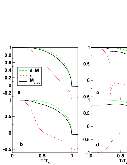
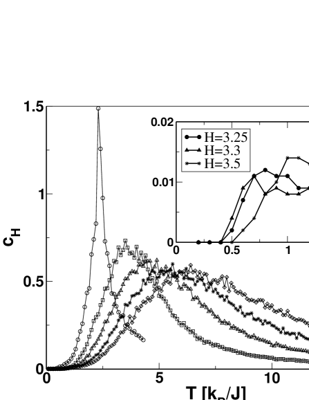
The solution of Eq. (12) versus temperature is plotted in Fig. 2 for different values of $\tilde{H}^{\prime}$. We see the characteristic reduction of the effective magnetization to $1-2/10=0.8$. This reduction occurs as long as $0.1+0.071=0.171<\mu_{0}H_{s}$ according to (9). Fig. 2(c) displays that slightly below the critical value ($\mu_{0}H_{s}=0.17$) we do not have a reduction at $T=0$ but a sharp drop of the magnetization around $T/T_{c}=2J^{\prime}/jJ=0.35$. This is related to a maximum in the specific heat at a second critical temperature $T_{c}^{\prime}\approx 0.35T_{c}$ besides the usual Ising transition temperature $T_{c}$ as shown in Fig. 3. The same second transition appears in Fig. 1 where $\mu_{0}H_{s}=5$ and consequently the reduction occurs as long as $\mu_{0}H<3.29$.

Figure 2: The mean spins $s$ (dashed line) and $s^{\prime}$ (dotted line) as solution of (12) versus temperature together with the total mean magnetization, M_step, (solid line) for $\mu_{0}H_{s}=0.10,0.16,0.17,0.18$ (a-d). The magnetization without step agrees with $s$. The lattice size is $N=10$, the couplings $J=0.1$ and $J^{\prime}=J/\sqrt{2}$, and the external field $H=0$.

IV Mean-field critical exponents of new transition

We can understand the second transition by expanding (12) for low fields $H$ and calculating the susceptibility

$$\chi={\partial M\over\partial H}|_{H=0}.$$ (14)

From (12) we obtain

$${\partial s^{\prime}\over\partial H}\! = \!\beta(1\!-\!s^{\prime 2})\left(\mu_{0}\!+\!({T_{c}\over j}+{T_{c}^{\prime}\over 2}){\partial s\over\partial H}\!+\!T_{c}^{\prime}{\partial s^{\prime}\over\partial H}\right)$$

$${\partial s\over\partial H} = \beta(1-s^{2})\left(\mu_{0}+T_{c}{\partial s\over\partial H}\right)$$ (15)

which is easily solved and employed to calculate (14). We discuss this susceptibility explicitly near the two transitions. At the usual phase transition $T_{c}=jJ/k_{B}$ where $s=0$ we have

$$\chi|_{s=0}\!\! = \!\!\left(\!{N\!-\!1\over N}\!-\!{1\!-\!s^{\prime 2}\over N}{T\!+\!\frac{1}{2}T_{c}^{\prime}\!+\!({1\over j}\!-\!1)T_{c}\over T\!-\!(1\!-\!s^{\prime 2})T_{c}^{\prime}}\right){\mu_{0}/k_{B}\over T\!-\!T_{c}}$$

$$\lim\limits_{N\to\infty}\chi|_{s=0}\!\! = \!{\mu_{0}/k_{B}\over T-T_{c}}$$ (16)

and the typical critical exponent $\gamma=1$ occurs for finite and infinite lattices. The step of the surface does not change the critical scaling of the susceptibility.

Near the second transition at $T_{c}^{\prime}=2J^{\prime}/k_{B}$ where $s^{\prime}=0$ we obtain

$$\chi|_{s^{\prime}=0} = {\mu_{0}\over k_{B}}\left({1-N\over N}{1-s^{2}\over T-(1-s^{2})T_{c}}\right.$$

$$+\left.{1\over N}{T+(1-s^{2})((1/j-1)T_{c}+\frac{1}{2}T_{c}^{\prime})\over(T-(1-s^{2})T_{c})(T-T_{c}^{\prime})}\right)$$

$$\lim\limits_{N\to\infty}\chi|_{s^{\prime}=0} = -{\mu_{0}(1-s^{2})/k_{B}\over T-(1-s^{2})T_{c}}$$ (17)

and for a finite lattice ($N<\infty$) we see that $\chi\sim 1/(T-T_{c}^{\prime})$. Consequently, at the second critical temperature, $T_{c}^{\prime}$, the susceptibility diverges and a sharp drop of magnetization occurs with the critical exponent $\gamma^{\prime}=1$. This second critical temperature does not appear for infinite lattices since the term with $1/(T-T_{c}^{\prime})$ vanishes in the limit $N\to\infty$. We hence conclude that the second transition occurs due to the finite spacing between two adjacent surface steps.

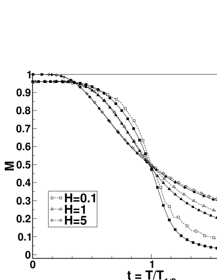
Even the quantitative behavior of the mean-field model agrees remarkably well with the numerical solution if we scale to the corresponding half-width temperatures as can be seen in Fig. 4. Especially the low-temperature behavior and the drop at the second, low-temperature transition at $T_{c}^{\prime}$ are well described. Since the mean-field approximation does not yield the correct critical exponents of the standard order-disorder transition of the planar two-dimensional Ising model it is in accordance with previous findings that deviations occur for temperatures higher than $T_{1/2}$.

Figure 3: The specific heat for parameters of Fig. 1 for the numerical data of the Ising model with a step.

In order to substantiate the picture of a second, low-temperature transition we investigate the remaining critical exponents. We find the magnetic field dependence of the magnetization by rewriting (12)

$${\mu_{0}H\over k_{B}T} = -{T_{c}\over T}s+\frac{1}{2}\ln\left({1+s\over 1-s}\right)$$ (18)

and near $T_{c}$

$${\mu_{0}H\over k_{B}T_{c}} = \frac{1}{3}\left({N\over N-1}M-{s^{\prime}\over N-1}\right)^{3}+o(s^{5})$$ (19)

where (13) has been used. We see that $\delta=0$ for finite lattices while for $N\to\infty$ we obtain the established value $\delta=3$ of the standard Ising model. In the same way we obtain near $T_{c}^{\prime}$

$${\mu_{0}(H\!-\!H_{s})\over k_{B}T_{c}^{\prime}}\! = \!-\!\left({T_{c}\over jT_{c}^{\prime}}+\frac{1}{2}\right)s\!-\!s^{\prime}\!+\!\frac{T}{2T_{c}^{\prime}}\ln\!\left({1\!+\!s^{\prime}\over 1\!-\!s^{\prime}}\right)$$ (20)

$$= \!-\left({T_{c}\over jT_{c}^{\prime}}+\frac{1}{2}\right){N\over N\!-\!1}M+o(s^{\prime})$$

and we see that in both, finite and infinite lattices (with $H_{s}=0$) we have $\delta^{\prime}=1$, which is different from the standard Ising model. The finite Ehrlich-Schwoebel barrier, $H_{s}\neq 0$, leads to $\delta^{\prime}=0$.

We find the spontaneous magnetization for $H=0$ near $T_{c}$ from (18)

$${T_{c}/T}=1+{s^{2}\over 3}+o(s^{4})$$ (21)

which results with (12) in

$$M={s^{\prime}\over N}+{N-1\over N}\sqrt{3\left({T_{c}\over T}-1\right)}$$ (22)

such that we have $\beta=\frac{1}{2}$ for the infinite-size limit and $\beta=0$ for the finite-size case. Near $T_{c}^{\prime}$ we obtain analogously ${-\mu_{0}H_{s}}+(\frac{1}{j}T_{c}+\frac{1}{2}T_{c}^{\prime})s+{T_{c}^{\prime}}s^{\prime}=s^{\prime}T+o(s^{\prime 3})$ which leads to

$$\!M\!=\!\frac{N\!-\!1}{N}{T\!-\!T_{c}^{\prime}\over\frac{1}{j}T_{c}\!+\!\frac{1}{2}T_{c}^{\prime}}s^{\prime}\!+\!\frac{1}{N}s^{\prime}\!+\!{N\!-\!1\over N}{\mu_{0}H_{s}\over k_{B}(\frac{1}{j}T_{c}\!+\!\frac{1}{2}T_{c}^{\prime})}$$ (23)

and $\beta^{\prime}=0$ for finite-size lattices independent of the Ehrlich-Schwoebel barrier. The same exponent appears for infinite size since according to (13) the anomalous spins $s^{\prime}$ do not contribute to the magnetization in the infinite limit.

Figure 4: The magnetization of the Ising model (open symbols and dashed line) with a step as in Fig. 1, together with the solution of (12) (closed symbols and solid lines).

Besides the divergence at $T_{c}$ the specific heat shows a second maximum at $T_{c}^{\prime}=2J^{\prime}/JT_{c}$ for fields fulfilling (9) as can be seen in Fig. 3. The interesting leading order near the critical points at $H=0$, where we have $s=\sqrt{3(T_{c}/T-1)}$ from (21), reads

$$c_{H}/k_{B}={\sqrt{3}(N-1)s^{\prime}T_{c}^{3/2}(\frac{1}{j}T_{c}+\frac{1}{2}T_{c}^{\prime})\over 4N^{2}(T_{c}-(1-s^{\prime 2})T_{c}^{\prime})}{1\over(T_{c}-T)^{3/2}}$$

$$+{o(\frac{1}{N})\over T\!-\!T_{c}}\!+\!{o(\frac{1}{N})\over\sqrt{T\!-\!T_{c}}}\!-\!\frac{9}{8}\!+\!o(\frac{1}{N})\!+\!o(\sqrt{T-T_{c}})$$ (24)

which leads to $\alpha=3/2$ for the finite and $\alpha=0$ for the infinite case. Near the other critical point $T_{c}^{\prime}$ with $s^{\prime}\to 0$ we have the leading order

$${c_{H}^{\prime}\over k_{B}} = {({\mu_{0}\over k_{B}}H_{s})^{2}(1\!-\!N)[a\!+\!T_{c}^{\prime}(2T_{c}\!+\!jT_{c}^{\prime})^{2}]^{2}\over a^{2}N^{2}(T\!-\!T_{c}^{\prime})^{2}}\!+\!{o(\frac{1}{N})\over T\!-\!T_{c}^{\prime}}$$ (25)

$$+ ({2\mu_{0}\over k_{B}}H_{s}jT_{c})^{2}[({2\mu_{0}\over k_{B}}H_{s}j)^{2}-(2T_{c}\!+\!jT_{c}^{\prime})^{2}]$$

$$\times {a\!\!+\!\!2(T_{c}\!\!-\!\!T_{c}^{\prime})(2T_{c}\!\!+\!\!jT_{c}^{\prime})^{2}\over a^{3}}\!+\!o(\frac{1}{N})\!+\!o(T\!-\!T_{c}^{\prime})$$

with $a=-4\mu_{0}^{2}H_{s}^{2}j^{2}T_{c}/k_{B}^{2}+(T_{c}-T_{c}^{\prime})(2T_{c}+jT_{c}^{\prime})^{2}$. It shows $\alpha^{\prime}=2$ for the finite case and $\alpha^{\prime}=0$ for the infinite case. In the case with no Ehrlich-Schwoebel barrier ($H_{s}=0$) the specific heat becomes $c_{H}^{\prime}\sim o(s^{\prime 2})$ which shows $\alpha^{\prime}=0$, and no second transition $s^{\prime}=0$ occurs for finite or infinite systems.

	$\alpha$	$\beta$	$\gamma$	$\delta$	$\alpha\!\!+\!\!2\beta\!\!+\!\!\gamma$	$\alpha\!\!+\!\!\beta(1\!\!+\!\!\delta)$
2D Ising (exact)	0	1/8	7/4	15	2	2
2D Ising (Weiss)	0	1/2	1	3	2	2
$T_{c}$ $N\!\neq\!\infty$	3/2	0	1	0	2.5	1.5
$T_{c}$ $N\!=\!\infty$	0	1/2	1	3	2	2
$T_{c}^{\prime}$ $N\!\neq\!\infty$ ($H_{s}\!=\!0$)	2 (0)	0 (0)	1 (1)	0 (1)	3 (1)	2 (2)
$T_{c}^{\prime}$ $N\!=\!\infty$ ($H_{s}\!=\!0$)	0 (0)	0 (0)	0 (0)	0 (1)	0 (0)	0 (0)

Table 1: Critical exponents for the two transitions in mean-field approximation. The value in brackets give the results without Ehrlich-Schwoebel barrier.

One should note that the divergence of the specific heat appears here in the mean-field model though the numerical data show a mere maximum. This rounding of the divergence is due to the finite size of the lattice and well discussed, see [Fisher and Ferdinand, 1967].

The results for the mean-field model are summarized in table 1. We see that for infinite lattices the presence of the step does not change the exponents of the Ising model near the normal transition $T_{c}$. The finite-size effects lead to a deviation of all exponents from the result without step except the exponent of the susceptibility which remains unchanged. Especially the specific heat changes from logarithmic divergence to power-law divergence. For the reported second transition the scaling inequalities are fulfilled. In the infinite-size limit no second transition occurs.

Please note that we compare here the mean-field critical exponents for the new transition arising due to the Ehrlich-Schwoebel barrier. The exact one for the ladder defects without Ehrlich-Schwoebel barrier is well known Bariev (1979), as presented above (2).

V Summary

For Ising systems on a square lattice with a spatial distortion we report here that a second, low-temperature transition occurs besides the standard Ising phase transition. An analytical two-spin model is capable to describe the main features of such a distorted finite spin system. The divergent heat capacity appears here due to the spatial distortion and not due to an Ising phase transition. Therefore, experimentally recorded signals with divergent heat capacities may not exclusively be interpreted in terms of phase transitions in finite systems. When simulating the surface coverage with molecules the present model is able to describe the main equilibrium features Loppacher et al. (2006), thus it promises an application potential to the fabrication of nanowires which are created near a surface step.

Appendix A Critical Ehrlich-Schwoebel barrier

Here we outline the discussion of the critical Ehrlich-Schwoebel barrier where the second transition occurs in a two-spin model if condition (9) is fulfilled. A completely analogous discussion leads to the result for the three-spin model (7).

The fictitious spin $s^{\prime}$ obeys the equation

$$s^{\prime}={\rm tanh}\beta(H-H_{s}+as+bs^{\prime})$$ (26)

and the second transition occurs if $s=1$ and $s^{\prime}=-1$ since only in this case the magnetization (13) is reduced. For zero temperature the ${\rm tanh}$ function shows that $s^{\prime}=\pm 1$ if and only if

$$c_{\pm}=H+a\pm b\gtrless H_{s}.$$ (27)

Since $c_{-}<c_{+}$ we have the situation that for $H_{s}<c_{-}$ we have $s^{\prime}=1$ and for $H_{s}>c_{+}$ we have $s^{\prime}=-1$ while for $c_{-}<H_{s}<c_{+}$ both solutions $s^{\prime}=\pm 1$ exists. In this range the system will take the solution where the partition function becomes maximal. Since the partition function is proportional to ${\rm cosh}(c_{\pm}-H_{s})$ we have $s^{\prime}=\pm 1$ if

$$|c_{+}-H_{s}|\gtrless|c_{-}-H_{s}|.$$ (28)

Since we considered the range $c_{-}<H_{s}<c_{+}$ we obtain with (27)

$$H+a\gtrless H_{s}$$ (29)

as a unique condition where $s=1$ and $s^{\prime}=\pm 1$ and where the second transition occurs.

References

- Campi et al. (2005) X. Campi, H. Krivine, E. Plagnol, and N. Sator, Phys. Rev. C 71, 041601(R) (2005).
- Fisher and Ferdinand (1967) M. E. Fisher and A. E. Ferdinand, Phys. Rev. Lett. 19, 169 (1967).
- Chung et al. (2000) M. C. Chung, M. Kaulke, I. Peschel, M. Pleimling, and W. Selke, Eur. Phys. J. B 18, 655 (2000).
- Igloi et al. (1993) F. Igloi, I. Peschel, and L. Turban, Adv. in Phys. 42, 683 (1993).
- Loppacher et al. (2006) C. Loppacher, U. Zerweck, L. M. Eng, S. Gemming, G. Seifert, C. Olbrich, K. Morawetz, and M. Schreiber, Nanotechnology 17, 1568 (2006).
- Kumar et al. (1983) A. Kumar, H. R. Krishnamurthy, and E. S. R. Gopal, Phys. Rep. 98, 57 (1983).
- Onsager (1944) L. Onsager, Phys. Rev. 65, 117 (1944).
- Yang (1952) C. N. Yang, Phys. Rev. 85, 808 (1952).
- Abraham (1973) D. B. Abraham, Phys. Lett. 43, 163 (1973).
- Gaunt and Domb (1970) D. S. Gaunt and C. Domb, J. Phys. C 3, 1442 (1970).
- Jones and March (1973) W. Jones and N. H. March, Theoretical Solid State Physics, vol. 2 (Dover, New York, 1973).
- Rushbrooke (1963) G. S. Rushbrooke, J. Chem. Phys. 39, 842 (1963).
- Griffiths (1965) R. B. Griffiths, Phys. Rev. Lett. 14, 623 (1965).
- Kadanoff (1990) L. P. Kadanoff, Physica A 163, 1 (1990).
- Back et al. (1995) C. H. Back, C. Würsch, A. Vaterlaus, U. Ramsperger, U. Maler, and D. Pescia, Nature 378, 597 (1995).
- Rikvold et al. (1994) P. A. Rikvold, H. Tomita, S. Miyashita, and S. W. Sides, Phys. Rev. E 5080, 49 (1994).
- Korniss et al. (2000) G. Korniss, C. J. White, P. A. Rikvold, and M. A. Novotny, Phys. Rev. E 63, 016120 (2000).
- Binder and Hohenberg (1974) K. Binder and P. C. Hohenberg, Phys. Rev. B 9, 2194 (1974).
- Mills (1971) D. L. Mills, Phys. Rev. B 3, 3887 (1971).
- McCoy and Perk (1980) B. M. McCoy and J. H. H. Perk, Phys. Rev. Lett. 44, 840 (1980).
- Ko et al. (1985) L. F. Ko, H. Au-Yang, and J. H. H. Perk, Phys. Rev. Lett. 54, 1091 (1985).
- Kadanoff (1981) L. P. Kadanoff, Phys. Rev. B 24, 5382 (1981).
- Bariev (1979) R. Z. Bariev, Soviet Phys. JETP 50, 613 (1979).
- Brown (1982) A. C. Brown, Phys. Rev. B 25, 331 (1982).
- Bariev (2000) R. Z. Bariev, Braz. J. Phys. 30, 680 (2000).
- Schinzer et al. (2000) S. Schinzer, S. Köhler, and G. Reents, Eur. Phys. J. B 15, 161 (2000).