Excitation spectra of the spin-$1/2$ triangular-lattice Heisenberg antiferromagnet

Abstract

We use series expansion methods to calculate the dispersion relation of the one-magnon excitations for the spin-$1/2$ triangular-lattice nearest-neighbor Heisenberg antiferromagnet above a three-sublattice ordered ground state. Several striking features are observed compared to the classical (large-$S$) spin-wave spectra. Whereas, at low energies the dispersion is only weakly renormalized by quantum fluctuations, significant anomalies are observed at high energies. In particular, we find roton-like minima at special wave-vectors and strong downward renormalization in large parts of the Brillouin zone, leading to very flat or dispersionless modes. We present detailed comparison of our calculated excitation energies in the Brillouin zone with the spin-wave dispersion to order $1/S$ calculated recently by Starykh, Chubukov, and Abanov [cond-mat/0608002]. We find many common features but also some quantitative and qualitative differences. We show that at temperatures as low as $0.1J$ the thermally excited rotons make a significant contribution to the entropy. Consequently, unlike for the square lattice model, a non-linear sigma model description of the finite-temperature properties is only applicable at extremely low temperatures.

I Introduction

Spin-$1/2$ Heisenberg antiferromagnets on frustrated lattices constitute an important class of strongly correlated quantum many-body systems. The interest in these models has been particularly stimulated by the tantalizing possibility that the interplay between quantum fluctuations and geometric frustration might lead to a spin-liquid ground state and fractionalized (i.e., $S=1/2$) “spinon”excitations. By a spin liquid we mean a state which breaks neither translational nor spin rotational symmetry. This exotic scenario originated with the pioneering work by Anderson and Fazekas more than thirty years ago,andfaz where they suggested that a short-range resonating valence bond (RVB) state might be the ground state of the nearest-neighbor Heisenberg antiferromagnet on the triangular lattice. More recently, considerable progress has been made in understanding such states in terms of field theory and quantum dimer models.slreviews Whereas the existence of such a ground state and of spin-half excitations is well established in one dimension,giamarchi it is yet to be conclusively established theoretically in a realistic two-dimensional Heisenberg model.moso

Among the most important such models is the one considered by Anderson and Fazekas, namely the Heisenberg antiferromagnet on the triangular lattice with only nearest-neighbor (isotropic) exchange interactions (hereafter just referred to as the triangular-lattice model for brevity). However, over the past decade numerical studiesbernu94 ; singhhuse ; farnell ; capriotti99 using a variety of different techniques do not support the suggestion in Ref. andfaz, of a spin-liquid ground state for this model. Instead, they provide evidence that the ground state is qualitatively similar to the classical one, with noncollinear magnetic Néel order with a three-sublattice structure in which the average direction of neighboring spins differs by a 120 degree angle.

On the other hand, there are other theoretical results which suggest that some properties of this model are indeed quite unusual. First, a short-range RVB state is found to have excellent overlap with the exact ground state for finite systems, much better than for the square lattice.sindzingre ; yunsor Second, variational calculations for RVB states, both with and without long range order, give very close estimates for the ground state energies.sindzingre ; yunsor Third, early zero-temperature series expansion studies found some evidence that this model may be close to a quantum critical point.singhhuse Fourth, one can make general arguments, based on the relevant gauge theoriesgauge that the quantum disordered phase of a non-collinear magnet should have deconfined spinons,read although in the ordered phase the spinons are confined.chubukov2 Finally, high-temperature series expansion studieselstner performed for temperatures down to $J/4$ ($J$ being the exchange interaction) found no evidence for the “renormalized classical” behavior that would be expected from a semiclassical nonlinear sigma model approach, if the ground state has long range order.nlsmtr ; css ; css2 The actual behavior (summarized in some detail in Sec. VII.1) is rather striking and is in stark contrast to the square-lattice model for which the “renormalized classical” behavior appears very robust.chn89

On the experimental side, there are currently no materials for which it has been clearly established that their magnetic properties can be described by the $S=1/2$ isotropic triangular-lattice Heisenberg antiferromagnet. In contrast, it has been clearly established that the one dimensional and square lattice Heisenberg models with only nearest-neighbour exchange give good descriptions of a number of materials. Examples of the former include KCuF₃tennant and Sr₂CuO₃,sandvik and of the latter Cu(DCOO)₂.4D₂O.mcmorrow For the triangular-lattice the most exciting prospect may be the organic compound $\kappa$-(BEDT-TTF)₂Cu₂(CN)₃,shimizu which is estimated from quantum chemistry calculations to have weak spatial anisotropykomatsu . Indeed comparisons of the thermodynamic susceptibility with the high temperature expansions calculated for a class of spatially anisotropic triangular-lattice models suggest that the system may actually be very close to the isotropic triangular-lattice Heisenberg model.zheng05hight In Section VIII.2 we review the recent experimental evidence that this material has a spin liquid ground state.

In this work we present series expansion calculations for the triangular-lattice model. The primary focus is on the dispersion relation of the magnon excitations above the 120-degree spiral-ordered ground state. A brief description of some of our results was presented in an earlier communication.zheng06 In this paper we discuss our results and the series expansion and extrapolation methods in more detail. We also compare our results quantitatively with very recent calculations of the spin-wave dispersion by Starykh et al.starykh based on nonlinear spin-wave theory which includes quantum corrections of order $1/S$ (to be called SWT+1/S results) to the classical large-$S$ or linear spin-wave theory (LSWT) results.

One of the most striking features of the spectrum is the local minimum in the dispersion at the six wave vectors in the middle of the faces of the edge of the Brillouin zone. Such a minimum is absent in the spectrum calculated in linear spin wave theory. In particular, along the edge of the Brillouin zone the semi-classical dispersion is a maximum, rather than a minimum at this point. This dip is also substantially larger than the shallow minima which occurs in the square lattice model. Hence, this unique feature seems to result from the interplay of quantum fluctuations and frustration. We have called this feature a “roton” in analogy with similar minima that occur in the excitation spectra of superfluid ⁴Hefeynman and the fractional quantum Hall effect.girvin In those cases, by using the single mode approximation for the dynamical structure factor one can see how the roton is associated with short range static correlations. Thus, an important issue is to ascertain whether this is also the case for the minima we consider here. Calculations of the static structure factor for the square lattice do not show a minima at the relevant wavevector.zheng04 We note that the roton we consider is quite distinct from the “roton minima” for frustrated antiferromagnets that has been discussed by Chandra, Coleman, and Larkinchandra . The effect they discuss only occurs for frustrated models which have large number of classically degenerate ground states not related by global spin rotations. If we apply their theory to the triangular lattice it does not predict such a minima. Finally, we note that anomalous roton minima also appear in the spectrum of the Heisenberg model with spatially anisotropic exchange constants on the triangular lattice in the regime where the magnetic order is collinear.zheng06 Such roton minima were also found in a recent study of an easy-plane version of the same model,alicea where the elementary excitations of the system are fermionic vortices in a dual field theory. In that case, the roton is a vortex-anti-vortex excitation making the “roton” nomenclature highly appropriate!

The spectra we have calculated show substantial deviations from the LSWT results, especially at high energies and for wavevectors close to the crystallographic zone boundary, emphasizing the importance of non-linear effects in the spin dynamics. Several features of our calculated spectra are captured by the nonlinear spin-wave theory,starykh but there are also quantitative and qualitative differences. Both calculations show a substantial downward renormalization of the classical spectra. However, the highest excitation energies in the Brillouin Zone are lowered with respect to LSWT by about $40\%$ in the series calculations compared to about $25\%$ in SWT+1/S results. Both calculations show substantial flat or nearly dispersionless spectra in large parts of the Brillouin Zone. However, the flat regions are much more pronounced in the series calculations near the highest magnon energies, whereas they are more pronounced at intermediate energies in SWT+1/S results. In the series calculations the magnon density of states (DOS) has an extremely sharp peak near the highest energies, whereas in the SWT+1/S calculations the largest peak in DOS is at intermediate energies. The roton-like minima at the mid-points of the crystallographic zone-boundary are much more pronounced in the series calculations. They are much weaker in the SWT+1/S results and are really part of the flat energy regions contributing to the largest DOS peak in the latter calculations.

The SWT+1/S calculations are much closer to series expansion results than LSWT and on this basis one can conclude that the anomalous results obtained in series expansions are perturbatively related to LSWT. In other words, a picture based on interacting magnons captures the single-magnon excitations, once the non-linearities are taken into account. Indeed, we find that, if we treat magnons as non-interacting Bosons and calculate their entropy from the DOS obtained in the series calculations, we get an entropy per spin of about $0.3$ at $T/J=0.3$, a value not far from that calculated in high temperature series expansions.elstner Furthermore, we find that the low energy magnons give the dominant contributions to the entropy only below $T/J\approx 0.1$. This provides a natural explanation for why the non-linear sigma model based description, which focusses only on the low energy magnons, must fail above $T/J=0.1$.

There remains, however, an important open question with regard to the spectra of this model. The question relates to the nature of the multi-particle continuum above the one-magnon states. In particular, how much spectral weight lies in the multi-particle continuum, and can it be described by an interacting-magnon picture, or is it better thought of in terms of a pair of (possibly interacting) spinons? This question is also related to the physical origin of the roton minima. We note that neutron scattering measurements have observed a substantial multi-particle continuum in the two-dimensional spin-1/2 antiferromagnet Cs₂CuCl₄coldea (which is related to the triangular lattice explored here, the main difference being that Cs₂CuCl₄ has spatially anisotropic exchange couplings). For that system nonlinear spin-wave theoryveillette ; dalidovich could not account quantitatively for the continuum lineshapes observed experimentally.

The plan of the paper is as follows. In Sec. II we present our model Hamiltonian. In Sec. III we discuss the series expansion methods used for studying zero-temperature properties including the excitation spectra. Tables of various series coefficients are also presented there. In Sec. IV we discuss series extrapolation techniques. After a short Sec. V about ground state properties, we present results for the magnon dispersion in Sec. VI, and compare them in detail with nonlinear spin-wave theory. In Sec. VII we consider how thermal excitation of the rotons affects thermodynamic properties at much lower temperatures than might be expected, in analogy with superfluid ⁴He. We show how this can explain the absence of the renormalized classical behavior at finite temperatures, well below $T=J/4$. In Sec. VIII we discuss a possible interpretation of the roton in terms of confined spinon-anti-spinon pairs and the relevance of our results to experiments on $\kappa$-(BEDT-TTF)₂Cu₂(CN)₃. Finally, our conclusions are given in Sec. IX.

II Model

We consider an antiferromagnetic $S=1/2$ Heisenberg model on a triangular lattice. More precisely we will analyze a 2-parameter Hamiltonian of this type, given by

$$H=J_{1}\sum_{<in>}\bm{S}_{i}\cdot\bm{S}_{n}+J_{2}\sum_{<ij>}\bm{S}_{i}\cdot\bm{S}_{j}.$$ (1)

Here the $\bm{S}_{i}$ are spin-$1/2$ operators. The first sum is over nearest-neighbor sites connected by “horizontal” bonds (bold lines in Fig. 1) and exchange interaction $J_{1}$, the second sum is over nearest-neighbor sites connected by “diagonal” bonds (thin lines in Fig. 1) with exchange interaction $J_{2}$. As far as results are concerned, in this paper our focus is on the isotropic model defined by $J_{1}=J_{2}\equiv J$, but we find it convenient to distinguish between $J_{1}$ and $J_{2}$ for the purpose of making our discussion of the series expansion (Sec. III) method more general.

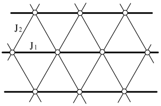
Figure 1: Exchange interactions in the Heisenberg model (1) on the triangular lattice. In this paper we focus on results for the case $J_{1}=J_{2}\equiv J$.

III Series expansions

In order to develop series expansions for the model in the ordered phase, we assume that the spins order in the $xz$ plane, with an angle $q$ between neighbors along $J_{2}$ bonds and an angle $2q$ along the $J_{1}$ bonds. The angle $q$ is considered as a variable; the actual value of $q$ is that which minimizes the ground state energy. We rotate all the spins so as to have a ferromagnetic ground state, with the resulting Hamiltonian: zheng04 ; advphys ; book

$$H=H_{1}+J_{1}H_{2}+J_{2}H_{3}$$ (2)

where

$$H_{1}=J_{1}\cos{(2q)}\sum_{<in>}S^{z}_{i}S^{z}_{n}+J_{2}\cos{(q)}\sum_{<ij>}S^{z}_{i}S^{z}_{j},$$ (3)

$$H_{2}=\sum_{<in>}S_{i}^{y}S_{n}^{y}+\cos{(2q)}S_{i}^{x}S_{n}^{x}+\sin{(2q)}(S_{i}^{z}S_{n}^{x}-S_{i}^{x}S_{n}^{z}),$$ (4)

$$H_{3}=\sum_{<ij>}S_{i}^{y}S_{j}^{y}+\cos{(q)}S_{i}^{x}S_{j}^{x}+\sin{(q)}(S_{i}^{z}S_{j}^{x}-S_{i}^{x}S_{j}^{z}).$$ (5)

We introduce the Heisenberg-Ising model with Hamiltonian

$$H(\lambda)=H_{0}+\lambda V$$ (6)

where

$$H_{0}=H_{1}-t\sum_{i}(S_{i}^{z}-1/2),$$ (7)

$$V=J_{1}H_{2}+J_{2}H_{3}+t\sum_{i}(S_{i}^{z}-1/2).$$ (8)

The last term of strength $t$ in both $H_{0}$ and $V$ is a local field term, which can be included to improve convergence. At $\lambda=0$, we have a ferromagnetic Ising model with two degenerate ground states. At $\lambda=1$, we arrive at our Heisenberg Hamiltonian of interest. We use linked-cluster methods to develop series expansion in powers of $\lambda$ for ground state properties and the magnon excitation spectra. The ground state properties are calculated by a straightforward Rayleigh-Schrödinger perturbation theory. However, the calculation of the magnon excitation requires new innovations compared to a case of collinear order. Since $S^{z}$ is not a conserved quantity here due to the last terms in Eqs. (4) and (5), the one-magnon state and the ground state belong to the same sector. The linked-cluster expansion with the traditional similarity transformationgel96 fails, as it allows an excitation to annihilate from one site and reappear on another far away, violating the assumptions for the cluster expansion to hold. To get a successful linked-cluster expansion, one needs to use the multi-block orthogonality transformation introduced in Ref. zhe01, . Indeed, we find that with proper orthogonalization the linked-cluster property holds.

The series for ground state properties have been computed to order $\lambda^{13}$, and the calculations involve a list of 4 140 438 clusters, up to 13 sites. These extend previous calculationssinghhuse by two terms, and are given in Table 1. Since, we are working here with a model that has the full symmetry of the triangular lattice, the series for the magnon excitation spectra can be expressed as:

$$\Delta(k_{x},k_{y})/J=\sum_{r=0}^{\infty}\lambda^{r}\sum_{m,n}c_{r,m,n}{\Big{[}}\cos(\frac{m}{2}k_{x})\cos(\frac{n\sqrt{3}}{2}k_{y})$$ (9)

$$+ \cos(k_{y}\sqrt{3}(m+n)/4)\cos(k_{x}(m-3n)/4)$$

$$+ \cos(k_{y}\sqrt{3}(m-n)/4)\cos(k_{x}(m+3n)/4){\Big{]}}/3$$

This series has been computed to order $\lambda^{9}$, and the calculations involve a list of 38959 clusters, up to 10 sites. The series coefficients $c_{r,m,n}$ for $t=1$ are given in Table 2.

IV Series extrapolations

In this section we discuss some details of the series extrapolation methods used in our analysis. In order to get the most out of the series expansions we have adopted a number of strategies. The convergence of the series depends on the parameter $t$. This parameter is varied to find a range where there is good convergence over large parts of the Brillouin zone. However, the naive sum of the series is never accurate at points where the spectra should be gapless. This is true for any model and its reasons are explained below.

We have found it useful to also develop series for the ratio of our calculated dispersion $\Delta(\bm{k})$ to the classical (large-S) dispersion $\Delta_{\rm{LSW}}(\bm{k})$ obtained from linear spin-wave theory. Following Ref. merino, , $\Delta_{\rm{LSW}}(\bm{k})$ for arbitrary $\lambda$ and $t$ is given by

$$\Delta_{\rm{LSW}}(\bm{k})=2S\sqrt{(\lambda A+C)(\lambda B+C)}$$ (10)

where

$$A = J_{1}\cos(k_{x})+2J_{2}\cos(k_{x}/2)\cos(\sqrt{3}k_{y}/2),$$

$$B = J_{1}\cos(k_{x})\cos(2q)$$

$$+ 2J_{2}\cos(\frac{k_{x}}{2})\cos(\frac{\sqrt{3}}{2}k_{y})\cos(q),$$

$$C = 2t(1-\lambda)-J_{1}\cos(2q)-2J_{2}\cos(q).$$

We can expand $\Delta_{\rm{LSW}}(\bf{k})$ in powers of $\lambda$, and the ratio of our series expansion calculation $\Delta(\bf{k})$ to the series for this linear spin-wave energy $\Delta_{\rm{LSW}}(\bf{k})$ will be called the ratio series for the rest of the paper. The naive sum of this ratio series appears to converge better because to get estimates for $\Delta(\bf{k})$ from it, we need to multiply the sum by the classical energy $\Delta_{\rm{LSW}}(\bf{k})$ and this ensures that both vanish at the same $\bf{k}$-points.

We have also done a careful analysis of the series using series extrapolation methods. By construction, the Hamiltonian $H(\lambda)$ has an easy-axis spin-space anisotropy for $\lambda<1$, which leads to a gap in the magnon dispersion. This anisotropy goes away in the limit $\lambda\to 1$ when the Hamiltonian becomes SU(2)-invariant. In this limit the gap must also go away as long as the ground state breaks SU(2) symmetry. This closing of the gap is known to cause singularities in the series. The singularities are generally weak away from ordering wavevectors and gapless points, but are dominant near the ordering wavevector where the gap typically closes in a power-law manner in the variable $1-\lambda$.advphys ; book

We have used d-log Padé approximants and integrated differential approximants in our analysis. In general, these approximants represent the function of interest $f$ in a variable $x$ by a solution to a homogeneous or inhomogeneous differential equation, usually of first or second order, of the form

$$P_{K}(x){d^{2}f\over dx^{2}}+Q_{L}(x){df\over dx}+R_{M}(x)f+S_{T}(x)=0$$ (11)

where $P_{K}$, $Q_{L}$, $R_{M}$, $S_{T}$ are polynomials of degree $K$, $L$, $M$, $T$ respectively. The polynomials are obtained by matching the coefficients in the power series expansion in $x$ for the above equation. They are uniquely determined from the known expansion coefficients of the function $f$ and can be obtained by solving a set of linear equations. If $P_{K}$ and $S_{T}$ are set to zero, these approximants correspond to the well known d-log Padé approximants, which can accurately represent power-law behavior. Integrated differential approximants have the additional advantage that they can handle additive analytic or non-analytic terms which cause difficulties for d-log Padé approximants. It is also possible to bias the analysis to have singularities at predetermined values of $x$ with or without predetermined power-law exponents. Using such approximants, which enforce a certain type of predetermined behavior on the function, is called biased analysis. We refer the reader to Ref. book, for further details.

We found that the convergence near the ordering wavevector $Q$ (see Fig. 3), was particularly poor. We know that we must have gapless spectra at $k=Q$ and $k=0$ as long as there is long-range order in the system. Yet, most unbiased analysis gave a moderate gap at $k=Q$. The convergence is better near $k=0$, where unbiased analysis is consistent with very small values of the gap. This behavior near $Q$ may be some evidence that long-wavelength correlations are not fully captured by the available number of terms in the series.

V Ground state properties

In this section we briefly discuss results for two ground-state properties of the triangular-lattice model: the ground state energy per site $E_{0}/N$ and the Néel order parameter $M$ (i.e., the sublattice magnetization).

In Fig. 2 we show the extrapolated ground state energy as a function of the angle $q$ between nearest neigbor spins along $J_{2}$ bonds. Clearly the ground state energy is minimized when $q$ takes the classical value $2\pi/3$. The resulting value for the ground state energy is $E_{0}/N=-0.5502(4)J$, which compares well with results obtained from other methods (see Table 3).

The series for the order parameter $M$ is extrapolated assuming a square-root singularity at $\lambda=1$, i.e., we extrapolate the series in the variable $\delta=1-(1-\lambda)^{1/2}$ using integrated differential approximants. This leads to the estimate $M=0.19(2)$. This estimate is known to be sensitive to the choice of the power law.singhhuse Our value for $M$ shows good consistency with what is obtained from other methods (see Table 3).

Figure 2: The ground state energy per site $E_{0}/N$, as a function of the angle $q$ between nearest neighbor spins along $J_{2}$ bonds, for the triangular-lattice model (i.e., $J_{1}=J_{2}\equiv J$). The minimum energy is obtained when $q=2\pi/3$, the same as for the classical model.

Figure 3: Reciprocal space of the triangular lattice including the hexagonal first Brillouin zone. Squares denote ordering wavevectors, circles denote wavevectors of the “roton” minima. The labeled points have coordinates ${\rm O}=(0,0)$, ${\rm P}=(2\pi/3,0)$, ${\rm A}=(\pi,0)$, ${\rm B}=(\pi,\pi/\sqrt{3})$, ${\rm C}=(2\pi/3,2\pi/\sqrt{3})$, ${\rm Q}=(4\pi/3,0)$, and ${\rm E}=(0,\pi/\sqrt{3})$. Also shown is the path ABOCPQBE along which the magnon dispersion is plotted in Figs. 4 and 5.

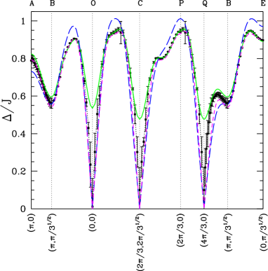
Figure 4: (Color online) Calculated spectra along ABOCPQBE of the Brillouin zone. Series extrapolation results (data points with error bars) are plotted together with naive sum of series with $t=2$ (green curve) and naive sum of ratio series with $t=1$ (blue dashed) and $t=2$ (magenta dashed).

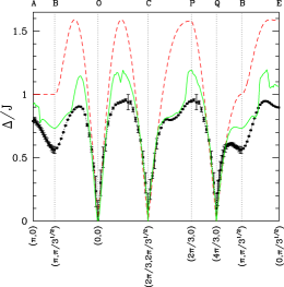
Figure 5: (Color online) Magnon spectra along ABOCPQBE from series expansions compared with LSWT (dashed red line) and SWT+1/S (green line).

VI Excitation spectra

The triangular-lattice Brillouin zone with selected wavevectors is shown in Fig. 3. In Fig. 4 we plot our most carefully extrapolated spectra along selected directions of the Brillouin zone using integrated differential approximants with appropriate biasing near the gapless points. The error bars are a measure of the spread in the extrapolated values from different approximants. Also shown in figure are the results from naive summation of the series as well as naive summation of the ratio series (see section IV) with two different $t$ values. In Fig. 5 we plot the series expansion results together with LSWT and SWT+1/S spectra.

The comparisons in Fig. 4 show that the substantial depression in the spin-wave energies obtained in the series expansions, over large parts of the Brillouin zone, is a very robust result that does not depend on extrapolations. Roton-like minima at wavevector B is also a very robust result already present in naive summation of the series. On the other hand, series extrapolations are essential near gapless points O, C, and Q. Even though the ratio series gives gapless excitations at these points, it does not get the spin-wave velocity right.

Since it is tedious to perform the full analysis of the spectra at all points of the Brillouin zone (and not necessary for the higher energy spectra), we have instead carried out a more restricted D-log Padé analysis over the whole zone. In Fig. 6 we show a two-dimensional projection plot of the spectra in the full Brillouin Zone. The color-code is adopted to highlight the higher energy part of the spectra, where our results should be most reliable, and minimize the variation at low energies where this analysis is not reliable. In Fig. 7, the corresponding two-dimensional projection plot for the SWT+1/S calculations are shown.

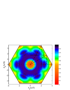
Figure 6: (Color online) Projection plot showing the magnon energies obtained from series expansions in the triangular-lattice Brillouin zone.

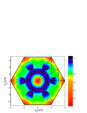
Figure 7: (Color online) Projection plot showing the SWT+1/S magnon energies in the triangular-lattice Brillouin zone.

In Fig. 8, we show the density of states (DOS) obtained from series analysis, LSWT and SWT+1/S. In each case the integrated density of states is normalized to unity.

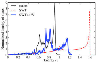
Figure 8: (Color online) Plots of magnon density of states for the series expansions, LSWT and SWT+1/S spectra.

From these plots, we make the following observations:

1. The SWT+1/S results share many common features with the series expansion results. Over most of the Brillouin zone the SWT+1/S results fall in between LSWT and series expansion results. They show that quantum fluctuations lead to substantial downward renormalization of the higher energy magnon spectra. This is in contrast to unfrustrated spin models, such as square-lattice or linear chain models, where quantum fluctuations lead to increase in excitation energies.

2. There are quantitative differences in the downward renormalization. The highest magnon energies are lowered with respect to LSWT by about $40\%$ in the series results and by about $25\%$ in SWT+1/S results.

3. The agreement in the low energy spectra and the spin-wave velocities is good when SWT+1/S results are compared to the biased integrated differential approximant analysis of the series.

4. Both the series results and SWT+1/S results show relatively flat or dispersionless spectra over large parts of the Brillouin Zone. These lead to sharp peaks in the density of states. However, there are some qualitative and quantitative differences here. In the series results the flattest part of the spectra that gives rise to the largest peak in the DOS are near the highest energy. A second smaller peak in the DOS primarily gets contributions from the neighborhood of the roton minima. Both these regions are highlighted in Fig. 9. In contrast, in SWT+1/S results the peak in the DOS near the highest magnon energies is much smaller. The flattest part of the spectra in SWT+1/S calculations are from the region near the roton minima. These are highlighted in Fig. 10.

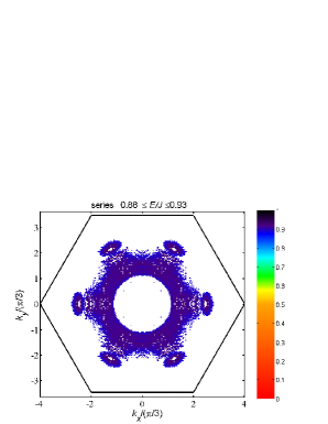
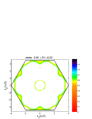
Figure 9: (Color online) Highlight of regions in the Brillouin zone that contribute to the DOS peaks in the series calculations.

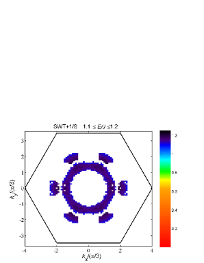
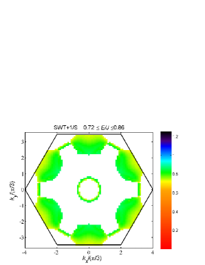
Figure 10: (Color online) Highlight of regions in the Brillouin zone that contribute to the DOS peaks in the SWT+1/S calculations.

5. The roton minima at wavevector B and equivalent points are present in both series expansion results and in SWT+1/S results. However, they are much more pronounced in the series results. A similar roton minima is seen in the square-lattice at ${\bf k}=(\pi,0)$, where it is also more prominent in series expansion and quantum Monte Carlo results,singh95 ; sylju1 ; sandvik3 absent in SWT+1/S results and barely visible in the next higher order spin-wave results.igarashi05

6. The two-dimensional plots for both series expansions and SWT+1/S have a similar look with a central annular high energy region, which is separated from 6 high energy lobes by a minima in the middle. The annular region in SWT+1/S appears more circular than in the series results, although both have clear hexagonal features. The lobes also have some differences.

7. The SWT+1/S calculations also predict finite lifetimes for spin-waves living around the center of the Brillouin Zone. These have not been taken into account in the series calculations and may also contribute to the difference between the two spectra.

Overall the comparison shows that the SWT+1/S results have many common features but also some differences. Neutron scattering spectra on a triangular-lattice material would be very exciting to compare with. In the meanwhile, sharp peaks in DOS may already be singled out in optical measurements. Given the qualitative differences, such measurements should be able to differentiate bwteen the SWT+1/S and series results. However, such spectra would depend on various matrix elements, and it would be important to develop a detailed theory for Raman scattering for these systems.

VII Finite temperature properties

In this section we discuss the implications of the spectra we have calculated, particularly the rotons, to properties of the triangular lattice model at finite temperatures. To emphasize the importance of this issue we first discuss the renormalized classical behavior expected at low temperatures for two-dimensional quantum spin systems, and the results of earlier high temperature series expansions which suggested otherwise.

VII.1 Finite-temperature anomalies

For a two-dimensional quantum spin system with an ordered ground state, the low temperature behavior should correspond to a Renormalized Classical (RC) one, that is a “classical” state with interacting Goldstone modes which is captured by the non-linear sigma model.chn89 It is instructive to compare the behavior of square and triangular lattices. Spin wave theory suggests that there are not significant differences between the quantum corrections for square and triangular lattice models at zero temperature. For both lattices, a diverse range of theoretical calculations suggest that the reductions in sublattice magnetization and spin-stiffness are comparable. If this is the case then one might expect Renormalized Classical behavior in the model to hold upto comparable temperatures. The relevant model for the square lattice is the O(3) model, and it has been very successful at describing both experimental results and the results of numerical calculations on the lattice model.chn89

For the triangular lattice, there are three Goldstone modes, two with velocity $c_{\perp}$ and one with velocity $c_{\parallel}$. The corresponding spin stiffnesses are denoted, $\rho_{\perp}$ and $\rho_{\parallel}$. Several different models have been suggested to be relevant, including O(3)xO(3)/O(2)nlsmtr and SU(2).css All of these models predict similar temperature dependences for many quantities.

In the large $N$ expansion, including fluctuations to order $1/N$ (the physical model has $N=2$), the static structure factor at the ordering wavevector iscss2

$$S(Q)\simeq 0.85\left({T\over 4\pi\rho_{s}}\right)^{4}\xi(T)^{2}$$ (12)

where the correlation length $\xi(T)$ (in units of the lattice constrant) is given bycaution

$$\xi(T)=0.021\left(c\over\rho_{s}\right)\left({4\pi\rho_{s}\over T}\right)^{1/2}\exp\left({4\pi\rho_{s}\over T}\right)$$ (13)

where $c=(2c_{\perp}+c_{\parallel})/3$ and $\rho_{s}=(2\rho_{\perp}+\rho_{\parallel})/3$ is the zero-temperature spin stiffness, which sets the temperature scale for the correlations. These expressions are quite similar to those for the $O(3)$ model that is relevant to the square lattice, with the $4\pi$ replaced by $2\pi$. An important prediction of equations (12) and (13) is that a plot of $T\ln(S(Q))$ or $T\ln(T\xi^{2}(T))$ versus temperature at low temperatures should increase with decreasing temperature and converge to a finite non-zero value which is proportional to the spin stiffness in the ordered state at zero temperature. Indeed, the relevant plots for the spin-1/2 square lattice modelelstner and the classical triangular lattice modelsouthern do show the temperature dependence discussed above. However, in contrast, the plots for the spin-1/2 model on the triangular lattice do not. In particular, $T\ln(S(Q))$ or $T\ln(T\xi^{2}(T))$ are actually decreasing with decreasing temperatureelstner down to $0.25J$. This is what one would expect if the ground state was actually quantum disordered with a finite correlation length at zero temperature. Hence, to be consistent with the ordered ground state at zero temperature these quantities must show an upturn at some much lower temperature.

The zero temperature value of the spin stiffness has been estimated for the TLM by a variety of methods, as shown in Table 3. The values are in the range $0.06J$ to $0.09J$. For $\rho_{s}=0.06J$ and $c=Ja$ taken from non-linear spin wave theory (also consistent with the dispersion relation found by series expansions), Equation (13) implies that the correlation length should be about 0.6 and 12 lattice constants at temperatures of $T=J$ and $T=0.25J$, respectively. For comparison, the high temperature series expansions giveelstner values of about 0.5 and 1.5 lattice constants, at $T=J$ and $T=0.25J$, respectively. It should be noted that the definitions of the correlation length in the field theory and in the series expansions is slightly different.css2

Furthermore, the entropy for the non-linear sigma model at low temperatures is just that of non-interacting bosons in two dimensions,

$$s(T)=\mathcal{A}\left({1\over c_{\parallel}^{2}}+{2\over c_{\perp}^{2}}\right)T^{2}+O(T^{4})$$ (14)

where $\mathcal{A}$ is a dimensionless constant of O(1). SWT+1/S gives $c_{\parallel}=1.11J$ and $c_{\perp}=0.69J$.css2 ; chubukov This means that for $T\ll J$ the system should have very small entropy. Indeed for the square lattice this is the case: it is about 0.05 at $T=0.3J$. Quantum Monte Carlo calculations found that for $T<0.25J$ the internal energy for the square lattice had the corresponding $T^{3}$ dependence.troyer However, for the triangular lattice the entropy is still 0.3 at $T=0.3J$. Chubukov, Sachdev, and Senthil,css2 suggested that the origin of the above discrepencies was related to a crossover between quantum critical and renormalised classical regimes. Previously, we suggestedzheng06 that the above discrepancies could be explained if one considered the rotons to be composed of a spinon and anti-spinon which were excited thermally. However, we now show how thermal excitations of rotons can explain the above discrepencies. There is a significant analogy here with the role that rotons play in superfluid ⁴He where they start to make substantial contributions to the entropy at temperatures much less than the roton gap.thanks ; fig-roton

VII.2 Contributions of rotons to finite temperature properties

We will calculate the entropy of the triangular-lattice model by assuming that the magnon excitations can be treated as a gas of noninteracting bosons with a dispersion as obtained from the series calculations. The entropy per site for noninteracting bosons (measured in units of $k_{B}=1$) is given by

$$s(T)=\int_{0}^{\infty}d\varepsilon\;g(\varepsilon)\;\Bigg{[}\frac{\varepsilon/T}{e^{\beta\varepsilon}-1}-\ln\Big{(}1-e^{-\beta\varepsilon}\Big{)}\Bigg{]}$$ (15)

where the DOS $g(\varepsilon)$ is normalized to unity. A plot of this entropy calculated from the series DOS in Fig. 8 is shown in Fig. 11. It is seen that the entropy is in fact larger than 0.3 at $T=0.3J$ and thus consistent with the high-temperature series data. It is also clear that the contribution to the entropy from the rotons/high-energy excitations (energy $\simeq 0.5$ and above) starts dominating over the contribution from the low-energy Goldstone modes at a temperatures slightly above $T=0.1J$ which is only about 1/5 of the roton gap. This shows that for the triangular lattice model the presence of rotons significantly influences thermodynamic properties even at very low temperatures and thus provides an explanation of why the finite-temperature behavior of the triangular-lattice model are very different from the square lattice model. In particular it implies that a nonlinear sigma-model description will be valid only at very low temperatures.

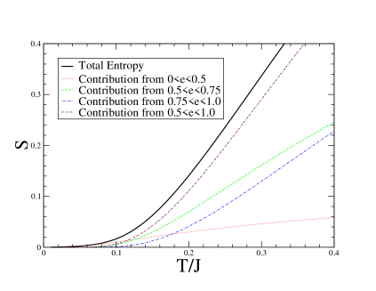
Figure 11: Entropy of the triangular-lattice Heisenberg model due to the magnon excitations. Contributions to the entropy from different energy ranges are shown. The low energy magnons only dominate the entropy below $T=0.1J$.

VIII Discussion

We have seen that SWT+1/S results for the spectra share many features of the series expansion results. Furthermore, the existence of rotons and flat-regions in the spectra at fairly low energies (about 4-times lower than for the square-lattice), gives a natural explanation for why the results of high-temperature series expansions for the square and triangular lattice models are qualitatively different. However, there are still some important questions to be addressed. First, we should stress that we still lack a physical picture (such as exists for superfluid ⁴He, thanks to Feynmanfeynman ) of the nature of the rotons. Moreover, recent experimental results on $\kappa$-(BEDT-TTF)₂Cu₂(CN)₃, and recent variational RVB calculations with spinon excitations, raise further issues. We now briefly review these points.

VIII.1 Are magnons bound spinon-anti-spinon pairs?

In our earlier paperzheng06 we suggested a possible explanation of the ‘roton’ minima in the magnon dispersion relation in terms of a downward energy renormalization due to a level-repulsion from a higher-energy two-spinon continuum. This requires that the spinon dispersion have local minima at specific wave vectors. For the square-lattice model a similar interpretation, based on the $\pi$-flux phase,affmar was originally proposed by Hsuhsu (see also Ref. hoetal, ) to explain the minima observed at ($\pi,0$) in that case. For the triangular-lattice model, several RVB states have spinon excitations with minima at the required locations. For example, Lee and Fengleefeng and Ogataogata considered a Gutzwiller projected BCS state with $d_{x^{2}-y^{2}}+id_{xy}$ pairing symmetry in the Gutzwiller approximation. However, the variational energy of this state ($-0.484J$) is about 15 per cent higher than the best estimates of the true ground state energy (see Table 3). In contrast, the Gutzwiller projected BCS states recently studied by by Yunoki and Sorellayunsor using variational Monte Carlo have energies comparable to the best estimates of the ground state energy. In their study, a state which can be related to a short range RVB state, has very good variational energy, and has spinons with mean field dispersion relation

$$E(\bm{k})=\left(\mu^{2}+(\Delta)^{2}(\cos^{2}k_{1}+\cos^{2}k_{2}+\sin^{2}(k_{1}-k_{2}))\right)^{1/2}$$ (16)

where $k_{1}$ and $k_{2}$ are the components of $\bm{k}$ that are parallel to the reciprocal lattice vectors, $\bm{G}_{1}$ and $\bm{G}_{2}$, of the triangular lattice. This dispersion has local minima at the four wave vectors, $\bm{k}={1\over 4}\left(\pm\bm{G}_{1}\pm\bm{G}_{2}\right).$ Spinon-antispinon excitations which make up spin triplet excitations will then have local minima at the six points in the middle of the edges of the Brillouin zone, i.e., the location of the roton minima found in the series expansions.

VIII.2 Experimental results

We now review recent experimental results on the Mott insulating phase of $\kappa$-(BEDT-TTF)₂Cu₂(CN)₃. Very interestingly, this material does not show any magnetic long-range order down to the lowest temperature studied, 32 mK,shimizu despite the fact that this temperature is four orders of magnitude smaller than the exchange interactions estimated to be around 250 K.

The temperature dependence of the Knight shift and nuclear magnetic relaxation rate, $1/T_{1}$, associated with ¹³C nuclei which have a significant interaction with the electron spin density have also been measured for this material.kawamoto ; shimizu2 This is a particularly useful measurement because the relaxation rate gives a measure of the range of the antiferromagnetic correlations. The observed temperature dependence of the Knight shift is the same as that of the uniform magnetic susceptibility,shimizu as it should be. As the temperature decreases, the ratio $1/T_{1}T$ increases by a factor of about two from 300 K down to 10 K, at which it decreases by about thirty per cent down to 6 K. There is no sign of splitting of NMR spectral lines, as would be expected if long range order develops. In contrast, for $\kappa$-(BEDT-TTF)₂Cu₂[N(CN)₂]Cl material, $1/T_{1}T$ increases rapidly with decreasing temperature and exhibits a cusp at the Neel temperature, reflecting the diverging antiferromagnetic correlation length. Evidence for the existence of magnetic order, in the latter material, comes from the splitting of NMR lines at low temperatures.kawamoto0

The observed temperature dependence of $1/T_{1}T$ and the spin echo rate $1/T_{2}$ for $\kappa$-(BEDT-TTF)₂Cu₂(CN)₃ is distinctly different from that predicted by a non-linear sigma model in the renormalised classical regimecss , namely that $1/T_{1}T$ be proportional to $T^{5/2}\xi(T)$, and $1/T_{2}$ be proportional to $T^{3}\xi(T)$, where the correlation length is given by (13). In particular, if this material has a magnetically ordered state at low temperatures, then both $1/T_{1}T$ and $1/T_{2}$ should be increasing rapidly with decreasing temperature, not decreasing. In the quantum critical regime, close to a quantum critical point,css $1/T_{1}\sim T^{\eta}$ where $\eta$ is the anomalous critical exponent associated with the spin-spin correlation function. Generally, for O(n) sigma models, this exponent is much less than one. If $\eta>1$, as occurs for field theories with deconfined spinons,css ; alicea then $1/T_{1}T$ decreases with decreasing temperature, opposite to what occurs when the spinons are confined, because then $\eta\ll 1$.chn89 It is very interesting that at low temperatures, from 1 K down to 20 mK, it was foundshimizu2 that $1/T_{1}\sim T^{3/2}$ and $1/T_{2}\sim$ constant. In contrast for the materials described by the Heisenberg model on a square latticesandvik2 or a chain,sandvik both relaxation rates diverge as the temperature decreases. Hence, these NMR results are clearly inconsistent with a description of the excitations of this material in terms of interacting magnons. It is also observed that a magnetic field induces spatially non-uniform local moments.shimizu2 Motrunich has given a spin liquid interpretation of this observation.motrunich2 The simplest possible explanation of why these results at such low temperatures are inconsistent with what one expects for the nearest neighbour Heisenberg model is that such a model may not be adequate to describe this material and the spin liquid state may arise from the presence of ring exchange terms in the Hamiltonian.zheng05hight This has led to theoretical studies of such models.motrunich ; leelee

IX Conclusions

The present comparisons of the series results of the spectra with the order $1/S$ spin-wave theory suggests that the shape of the magnon dispersion relation can be understood in a more conventional picture of interacting magnons. Furthermore, the existence of the roton minima at points in the middle of the edges of the Brillouin zone and regions of flat dispersion in the zone, can explain why the low temperature properties of the triangular lattice model are so different from those of the square lattice. However, we still lack a clear physical picture for the nature of the rotons. An important issue to resolve is whether the most natural description for them is in terms of bound spinon-antispinon pairs.

From a theoretical point of view it may be interesting to add other destabilizing terms to the Hamiltonian, such as second neighbor interactions and ring-exchange terms, which can demonstrably lead to short correlation lengths and destabilize the 120 degree order, and then explore the changes in the dispersion relation, one-magnon weight and continuum lineshapes with variations in the model parameters.

It is also important to examine these results in the context of the organic material $\kappa$-(BEDT-TTF)₂Cu₂(CN)₃. The measured uniform susceptibility for this material shows excellent parameter-free agreement with the calculated susceptibility for the spin-1/2 triangular-lattice Heisenberg model. Yet, this system does not develop long-range order down to $T/J\approx 10^{-4}$.

Table 1: Series coefficients for the ground state energy per site $E_{0}/N$ and the order parameter $M$ for $t=0$ and $t=1$ for the isotropic triangular-lattice model ($q=2\pi/3$). Series coefficients of $\lambda^{n}$ up to order $n=13$ are listed.

$n$	$E_{0}/N$ for $t=0$	$E_{0}/N$ for $t=1$	$M$ for $t=0$	$M$ for $t=1$
0	-3.750000000$\times 10^{-1}$	-3.750000000$\times 10^{-1}$	5.000000000$\times 10^{-1}$	5.000000000$\times 10^{-1}$
1	0.000000000	0.000000000	0.000000000	0.000000000
2	-1.687500000$\times 10^{-1}$	-9.375000000$\times 10^{-2}$	-1.350000000$\times 10^{-1}$	-4.166666667$\times 10^{-2}$
3	3.375000000$\times 10^{-2}$	-3.125000000$\times 10^{-2}$	5.400000000$\times 10^{-2}$	-2.777777778$\times 10^{-2}$
4	-4.433705357$\times 10^{-2}$	-1.435119721$\times 10^{-2}$	-1.363457908$\times 10^{-1}$	-2.036471287$\times 10^{-2}$
5	2.042585300$\times 10^{-2}$	-9.090555800$\times 10^{-3}$	8.589755026$\times 10^{-2}$	-1.803575334$\times 10^{-2}$
6	-2.832908602$\times 10^{-2}$	-6.546903212$\times 10^{-3}$	-1.657631567$\times 10^{-1}$	-1.659741503$\times 10^{-2}$
7	3.153484699$\times 10^{-2}$	-4.684496998$\times 10^{-3}$	2.055368406$\times 10^{-1}$	-1.456148506$\times 10^{-2}$
8	-4.765982794$\times 10^{-2}$	-3.395880980$\times 10^{-3}$	-3.691101414$\times 10^{-1}$	-1.262324583$\times 10^{-2}$
9	6.850871690$\times 10^{-2}$	-2.535518092$\times 10^{-3}$	5.890651357$\times 10^{-1}$	-1.102173131$\times 10^{-2}$
10	-1.025445984$\times 10^{-1}$	-1.940417545$\times 10^{-3}$	-1.005494430	-9.680160168$\times 10^{-3}$
11	1.565521577$\times 10^{-1}$	-1.501987905$\times 10^{-3}$	1.700641966	-8.486511451$\times 10^{-3}$
12	-2.455267547$\times 10^{-1}$	-1.170051241$\times 10^{-3}$	-2.948749946	-7.416819496$\times 10^{-3}$
13	3.935047914$\times 10^{-1}$	-9.185872231$\times 10^{-4}$	5.156611906	-6.481274769$\times 10^{-3}$

Table 2: Series coefficients for the magnon dispersion for the isotropic triangular-lattice model, calculated for $t=1$ in Eqs. (7) and (8). Nonzero coefficients $c_{r,m,n}$ in Eq. (9) up to order $r=9$ are listed.

($r,m,n$)	$c_{r,m,n}$	($r,m,n$)	$c_{r,m,n}$	($r,m,n$)	$c_{r,m,n}$	($r,m,n$)	$c_{r,m,n}$
( 0, 0, 0)	2.500000000	( 7, 4, 0)	-2.092658337$\times 10^{-2}$	( 7, 8, 0)	-2.788171252$\times 10^{-3}$	( 8,12, 0)	1.247798114$\times 10^{-4}$
( 1, 0, 0)	-1.000000000	( 8, 4, 0)	-8.143627454$\times 10^{-2}$	( 8, 8, 0)	-3.352709547$\times 10^{-3}$	( 9,12, 0)	2.470018460$\times 10^{-4}$
( 2, 0, 0)	-4.988839286$\times 10^{-1}$	( 9, 4, 0)	-1.523543756$\times 10^{-2}$	( 9, 8, 0)	7.333948649$\times 10^{-3}$	( 7,12, 2)	2.937003840$\times 10^{-4}$
( 3, 0, 0)	-2.740918633$\times 10^{-1}$	( 3, 5, 1)	6.201171875$\times 10^{-2}$	( 5, 9, 1)	2.455267719$\times 10^{-3}$	( 8,12, 2)	1.899234898$\times 10^{-5}$
( 4, 0, 0)	-1.128855593$\times 10^{-2}$	( 4, 5, 1)	-4.072501106$\times 10^{-3}$	( 6, 9, 1)	-4.769602124$\times 10^{-4}$	( 9,12, 2)	-6.147374845$\times 10^{-5}$
( 5, 0, 0)	4.718452314$\times 10^{-2}$	( 5, 5, 1)	1.819088473$\times 10^{-2}$	( 7, 9, 1)	-1.354096601$\times 10^{-3}$	( 7,11, 3)	4.895006400$\times 10^{-4}$
( 6, 0, 0)	1.069731871$\times 10^{-2}$	( 6, 5, 1)	3.981234691$\times 10^{-2}$	( 8, 9, 1)	-5.219152848$\times 10^{-3}$	( 8,11, 3)	3.504866827$\times 10^{-4}$
( 7, 0, 0)	-2.783715438$\times 10^{-4}$	( 7, 5, 1)	-8.391751084$\times 10^{-3}$	( 9, 9, 1)	-9.505943368$\times 10^{-3}$	( 9,11, 3)	3.548457842$\times 10^{-4}$
( 8, 0, 0)	1.029634963$\times 10^{-2}$	( 8, 5, 1)	-4.326852838$\times 10^{-2}$	( 5, 8, 2)	4.910535438$\times 10^{-3}$	( 7,13, 1)	9.790012800$\times 10^{-5}$
( 9, 0, 0)	-7.409203681$\times 10^{-3}$	( 9, 5, 1)	1.194051895$\times 10^{-2}$	( 6, 8, 2)	2.089776036$\times 10^{-3}$	( 8,13, 1)	-1.697239410$\times 10^{-4}$
( 1, 2, 0)	7.500000000$\times 10^{-1}$	( 3, 6, 0)	1.033528646$\times 10^{-2}$	( 7, 8, 2)	-1.363667878$\times 10^{-3}$	( 9,13, 1)	-2.395827580$\times 10^{-4}$
( 2, 2, 0)	8.035714286$\times 10^{-2}$	( 4, 6, 0)	-2.807172967$\times 10^{-2}$	( 8, 8, 2)	-1.944215793$\times 10^{-3}$	( 7,14, 0)	6.992866286$\times 10^{-6}$
( 3, 2, 0)	-2.913527716$\times 10^{-1}$	( 5, 6, 0)	-4.880096703$\times 10^{-2}$	( 9, 8, 2)	2.068274612$\times 10^{-3}$	( 8,14, 0)	-5.264758087$\times 10^{-5}$
( 4, 2, 0)	-3.538253764$\times 10^{-1}$	( 6, 6, 0)	-3.117757381$\times 10^{-2}$	( 5,10, 0)	2.455267719$\times 10^{-4}$	( 9,14, 0)	-2.888908886$\times 10^{-5}$
( 5, 2, 0)	-1.433040888$\times 10^{-1}$	( 7, 6, 0)	1.625826764$\times 10^{-2}$	( 6,10, 0)	-7.192654350$\times 10^{-4}$	( 8,13, 3)	-1.415213825$\times 10^{-4}$
( 6, 2, 0)	6.032017508$\times 10^{-2}$	( 8, 6, 0)	2.418896967$\times 10^{-2}$	( 7,10, 0)	6.619708053$\times 10^{-5}$	( 9,13, 3)	-1.012838318$\times 10^{-4}$
( 7, 2, 0)	5.451813695$\times 10^{-2}$	( 9, 6, 0)	-3.062453544$\times 10^{-2}$	( 8,10, 0)	6.397714641$\times 10^{-4}$	( 8,14, 2)	-7.076069125$\times 10^{-5}$
( 8, 2, 0)	-4.427446338$\times 10^{-2}$	( 4, 7, 1)	-1.581420898$\times 10^{-2}$	( 9,10, 0)	-1.290395255$\times 10^{-3}$	( 9,14, 2)	1.239259101$\times 10^{-5}$
( 9, 2, 0)	-5.261673101$\times 10^{-2}$	( 5, 7, 1)	-1.015665919$\times 10^{-2}$	( 6,10, 2)	-1.311427742$\times 10^{-3}$	( 8,12, 4)	-8.845086406$\times 10^{-5}$
( 2, 3, 1)	-4.218750000$\times 10^{-1}$	( 6, 7, 1)	-1.671867122$\times 10^{-2}$	( 7,10, 2)	-3.880276886$\times 10^{-4}$	( 9,12, 4)	-8.553417963$\times 10^{-5}$
( 3, 3, 1)	1.425980548$\times 10^{-1}$	( 7, 7, 1)	-1.561157615$\times 10^{-2}$	( 8,10, 2)	4.062057862$\times 10^{-4}$	( 8,15, 1)	-2.021734036$\times 10^{-5}$
( 4, 3, 1)	2.239011724$\times 10^{-1}$	( 8, 7, 1)	1.139858035$\times 10^{-2}$	( 9,10, 2)	-1.607660184$\times 10^{-4}$	( 9,15, 1)	4.795929060$\times 10^{-5}$
( 5, 3, 1)	-8.857143618$\times 10^{-3}$	( 9, 7, 1)	3.929130986$\times 10^{-2}$	( 6,11, 1)	-5.245710967$\times 10^{-4}$	( 8,16, 0)	-1.263583772$\times 10^{-6}$
( 6, 3, 1)	-1.556426647$\times 10^{-1}$	( 4, 6, 2)	-1.186065674$\times 10^{-2}$	( 7,11, 1)	3.733048771$\times 10^{-4}$	( 9,16, 0)	1.192482027$\times 10^{-5}$
( 7, 3, 1)	-4.175359076$\times 10^{-2}$	( 5, 6, 2)	-1.432147845$\times 10^{-2}$	( 8,11, 1)	1.091608982$\times 10^{-3}$	( 9,15, 3)	3.763753619$\times 10^{-5}$
( 8, 3, 1)	1.015643471$\times 10^{-1}$	( 6, 6, 2)	-1.435136738$\times 10^{-2}$	( 9,11, 1)	1.851573788$\times 10^{-3}$	( 9,14, 4)	5.645630428$\times 10^{-5}$
( 9, 3, 1)	4.756044803$\times 10^{-2}$	( 7, 6, 2)	-5.307444139$\times 10^{-3}$	( 6, 9, 3)	-8.742851612$\times 10^{-4}$	( 9,16, 2)	1.613037265$\times 10^{-5}$
( 2, 4, 0)	-2.109375000$\times 10^{-1}$	( 8, 6, 2)	-6.778541366$\times 10^{-3}$	( 7, 9, 3)	-4.761605554$\times 10^{-4}$	( 9,17, 1)	4.032593163$\times 10^{-6}$
( 3, 4, 0)	-1.089232568$\times 10^{-1}$	( 9, 6, 2)	-2.509466719$\times 10^{-2}$	( 8, 9, 3)	-3.368803230$\times 10^{-4}$	( 9,18, 0)	2.240329535$\times 10^{-7}$
( 4, 4, 0)	8.339453634$\times 10^{-3}$	( 4, 8, 0)	-1.976776123$\times 10^{-3}$	( 9, 9, 3)	-8.706110790$\times 10^{-4}$
( 5, 4, 0)	1.053325085$\times 10^{-1}$	( 5, 8, 0)	3.310043485$\times 10^{-3}$	( 6,12, 0)	-4.371425806$\times 10^{-5}$
( 6, 4, 0)	9.023634592$\times 10^{-2}$	( 6, 8, 0)	2.627504861$\times 10^{-3}$	( 7,12, 0)	1.915360692$\times 10^{-4}$

Table 3: Ground state properties of the isotropic triangular-lattice model, obtained by different methods. $E_{0}/N$ is the energy per site (in units of $J$) for a system with $N$ lattice sites. The order parameter $M$ is the value of the expectation value of the spin in the ordered state. It would have a value of $0.5$ in the absence of quantum fluctuations, and is zero in a spin liquid ground state. $\rho_{s}$ is the average spin stiffness (in units of $J$) which in a non-linear sigma model description sets the temperature scale of the finite temperature properties. Note that some of the spin liquid states based on variational wave functions give values for the ground state energy comparable to the best estimates. DMRG, QMC, V, GF, and ED denote density matrix renormalisation group, Quantum Monte Carlo, Variational, Greens function, and Exact diagonalization, respectively. SRVB denotes short range RVB. GA denotes the Gutzwiller approximation. SB+1/N denotes Schwinger boson mean-field theory with 1/N fluctuations.

Method	Ref.	$N$	$E_{0}/N$	$M$	$\rho_{s}$
Series	this work	$\infty$	$-0.5502(4)$	$0.19(2)$
ED	runge,; bernu94,	$12$	$-0.6103$
		$36$	$-0.5604$	0.40
V SRVB	sindzingre,	$12$	$-0.6096$	0	0
		$36$	$-0.5579$	0	0
ED	lecheminant,	36			0.06
DMRG	xiang,	$\infty$	$-0.5442$
GFQMC	cap99,	$\infty$	$-0.5458(1)$	$0.205(10)$
VQMC, SRVB	yunsor,	$\infty$	$-0.5123$	$0$	0
VQMC, RVB	yunsor,	$\infty$	$-0.5357$	$0$	0
SWT+1/S	miy,	$\infty$	$-0.5466$	0.2497
SWT+1/S	chubukov,	$\infty$		0.266	0.087
d + id RVB GA	leefeng,	$\infty$	$-0.484(2)$	0	0
Coupled cluster	kruger,	$\infty$		0.2134	$\rho_{\parallel}=$ 0.056
SB+1/N	manuel,	$\infty$	-0.5533		$\rho_{\parallel}=$ 0.09