Partially incoherent gap solitons in Bose-Einstein condensates

Abstract

We construct families of incoherent matter-wave solitons in a repulsive degenerate Bose gas trapped in an optical lattice (OL), i.e., gap solitons, and investigate their stability at zero and finite temperature, using the Hartree-Fock-Bogoliubov equations. The gap solitons are composed of a coherent condensate, and normal and anomalous densities of incoherent vapor co-trapped with the condensate. Both intragap and intergap solitons are constructed, with chemical potentials of the components falling in one or different bandgaps in the OL-induced spectrum. Solitons change gradually with temperature. Families of intragap solitons are completely stable (both in direct simulations, and in terms of eigenvalues of perturbation modes), while the intergap family may have a very small unstable eigenvalue (nevertheless, they feature no instability in direct simulations). Stable higher-order (multi-humped) solitons, and bound complexes of fundamental solitons are found too.

I Introduction 

An ultracold Bose gas is, in general, a mixture of a coherent Bose-Einstein condensate (BEC) and an incoherent (fluctuating) “vapor”. As shown in Refs. HFB ; Vardi , the Hartree-Fock-Bogoliubov (HFB) description of such a mixture in one dimension is provided by the Gross-Pitaevskii (GP) equation for the condensate order parameter $\phi(x,t)$, coupled to equations for components of the vapor wave function, $u(x,t)$ and $v(x,t)$, which are responsible for normal and anomalous densities of the fluctuations. This approach and related formalisms for the description of fluctuations make it possible to analyze various effects, such as quantum phase diffusion in BEC and its depletion in a time-dependent trap through transfer of atoms to non-condensed states depletion , depletion of dark solitons depletion-dark , quantum-noise squeezing of gap solitons in a repulsive condensate trapped in an optical lattice (OL) Canberra , deviations from one-dimensionality Luca , and friction and diffusion of solitons in a cloud of thermal atoms friction . The full system of coupled HFB equations was used in Ref. Vardi to show that, in the case of attraction between atoms, the matter flux from the condensate to the vapor may lead to splitting of bright matter-wave solitons (which have been created experimentally in ⁷Li exper-bright and ⁸⁵Rb Cornish condensates) into two fragments that may be regarded as partially incoherent solitons, i.e., bound states of the coherent condensate and vapor components, similar to partially incoherent solitons known in nonlinear optics Moti .

The objective of this work is to find solutions for partially incoherent gap solitons (GSs) in an OL potential, and investigate their stability, at zero and finite temperatures. GSs in BEC were predicted using the GP equation GSprediction , and then created experimentally in a ⁸⁷Rb condensate gap_sol (these solitons were quite “meager”, each consisting of just a few hundred atoms). Partially incoherent lattice solitons at finite temperature ($T$) were qualitatively predicted in Ref. Ahufinger , which relied upon simulations of the GP equation, starting with a random Bose distribution at finite $T$ and gradually forming a soliton by switching the OL potential on. Families of two-component GSs of intragap and intergap types (see below), i.e., with chemical potentials of the components falling in one or different bandgaps of their common OL-induced linear spectrum, were found within the framework of GP equations coupled by repulsion between the species Gubeskys . It is relevant to mention that two-component solitons of the intergap type Moti2 , as well as their discrete counterparts Sukhorukov , were earlier predicted in lattice models of nonlinear optics Moti ; however, these were coherent objects and, unlike the model considered here (see below), they were found in models that did not include coherent four-wave-mixing terms.

The GS is not a ground state of the repulsive condensate (it is obvious that it does not realize an absolute energy minimum for the self-repulsive condensate loaded into the OL potential, with a given number of atoms), but it is nevertheless stable. It is relevant to stress the difference of the analysis of quantum fluctuations around the GSs from the problem of quantum depletion of dark solitons, where fluctuations fill out the notch at the center of the soliton and thus gradually destroy it depletion-dark . For GSs (which are bright solitons), the notch is absent in the family of solutions found in the first bandgap [see Fig. 2(a) below]. In the second gap, notch(es) may be present in decaying wings of the soliton’s waveform [see Figs. 2(b) and 5], but the soliton’s identity is not predicated on them.

The paper is organized as follows. In Section II, we formulate the model, which is based on time-dependent HFB equations for the coherent condensate and incoherent vapor components interacting with it (at finite $T$). Basic results for the partially coherent GS families of the intra- and intergap types, found in a numerical form at $T=0$ and $T>0$, are reported in Section III. Examples of higher-order (multi-humped) solitons of various types are presented in Section III too. Stability of these solitons is investigated, by means of computation of the corresponding eigenvalues for small perturbations, and in direct simulations, in Section IV. Section V concludes the paper.

II The model

Coupled time-dependent HFB equations are obtained as a truncation of a hierarchy of approximations HFB developed for the description of the dynamics of interacting condensate and vapor components of the degenerate bosonic gas, at very low but, generally, finite $T$. Following Ref. Vardi , the equations for the gas with repulsion between bosonic atoms are cast in the following normalized form, with the nonlinearity coefficient scaled to unity:

$$i\frac{\partial\phi}{\partial t}=-\frac{1}{2}\frac{\partial^{2}\phi}{\partial x^{2}}+\left[-\varepsilon\cos(2x)+\left|\phi\right|^{2}+2\tilde{n}\right]\phi+\tilde{m}\phi^{\ast},$$ (1)

$$i\frac{\partial}{\partial t}\left(\begin{array}[]{c}u\\ v\end{array}\right)=\left(\begin{array}[]{cc}\hat{L}&-\tilde{m}-\phi^{2}\\ \tilde{m}^{\ast}+(\phi^{\ast})^{2}&-\hat{L}\end{array}\right)\left(\begin{array}[]{c}u\\ v\end{array}\right).$$ (8)

Here $\hat{L}\equiv-(1/2)\partial_{xx}^{2}-\varepsilon\cos(2x)+2\left(\left|\phi\right|^{2}+\tilde{n}\right)$, $\tilde{n}\equiv\left(1+\mathcal{N}_{B}\right)\left|v\right|^{2}+\mathcal{N}_{B}|u|^{2}$ and $\tilde{m}\equiv-\left(1+2\mathcal{N}_{B}\right)uv^{\ast}$ are the normal and anomalous fluctuation densities (the asterisk stands for the complex conjugation),

$$\mathcal{N}_{B}=\left(e^{E/kT}-1\right)^{-1}$$ (9)

is the Bose occupancy, with $E$ the ground-state energy of the tight transverse confinement (note that the one-dimensional equations are derived from their 3D counterparts, assuming strong confinement in the transverse plane, by means of various approaches implying averaging in the transverse plane 3Dto1D ; Lev ), and $\varepsilon$ is the strength of the longitudinal OL potential, whose period is scaled to be $\pi$. A dynamical invariant of Eqs. (1-8) is the total number of atoms,

$$N=\int_{-\infty}^{+\infty}\left[2\left|\phi(x)\right|^{2}+\left(1+2\mathcal{N}_{B}\right)\left(\left|u(x)\right|^{2}+\left|v(x)\right|^{2}\right)\right]dx\equiv N_{\phi}(t)+N_{u}(t)+N_{v}(t)$$ (10)

(note that the expression for $N$ explicitly depends on $T$ via $\mathcal{N}_{B}$).

Partially incoherent GSs are looked for as bound states in which the coherent condensate and incoherent vapor components are trapped together in the OL,

$$\phi(x,t)=\Phi(x)e^{-i\mu_{\phi}t},\,\,\,\left\{u(x,t),v(x,t)\right\}=\left\{U(x)\,e^{-i\mu_{u}t},V(x)\,e^{+i\tilde{\mu}_{v}t}\right\},$$ (11)

with chemical potentials $\mu_{\phi}$, $\mu_{u}$ and $-\tilde{\mu}_{v}$ subject to the constraint (phase-locking condition),

$$\mu_{u}+\tilde{\mu}_{v}=2\mu_{\phi},$$ (12)

which implies that collisions may kick out pairs of condensate atoms into the vapor (i.e., dynamical depletion of the condensate); the above-mentioned transverse-confinement energy was subtracted from the chemical potentials. Equations for the stationary parts of the wave functions are obtained by the substitution of expressions (11) in Eqs. (1) and (8):

$$\mu_{\phi}\Phi = -\Phi^{\prime\prime}/2-\varepsilon\cos(2x)\Phi+\left(\left|\Phi\right|^{2}+2\tilde{n}\right)\Phi+\tilde{m}\Phi^{\ast},$$

$$\mu_{u}U = -U^{\prime\prime}/2-\varepsilon\cos(2x)U+2\left(\left|\Phi\right|^{2}+\tilde{n}\right)U-(\Phi^{2}+\tilde{m})V,$$

$$\tilde{\mu}_{v}V = -V^{\prime\prime}/2-\varepsilon\cos(2x)V+2\left(\left|\Phi\right|^{2}+\tilde{n}\right)V-\left(\Phi^{2}+\tilde{m}\right)^{\ast}U.$$ (13)

In the linear approximation, Eqs. (13) decouple into the Mathieu equation for the condensate, $\Phi^{\prime\prime}+2\left[\mu_{\phi}+\varepsilon\cos(2x)\right]\Phi=0$, and its replicas for $U$ and $V$, giving rise to identical bandgap spectra for the three waves. This bandgap spectrum is displayed, for the sake of illustration, in Fig. 1. GS solutions can be found if $\mu_{\phi}$, $\mu_{u}$ and $\tilde{\mu}_{v}$ [the latter chemical potential is equal to $-\mu_{u}+2\mu_{\phi}$, as per locking condition (12)] belong to one or different bandgaps. The respective solutions will be called intragap and intergap solitons, as in Ref. Gubeskys (see also Refs. Moti2 and Sukhorukov ). In particular, in the typical case of a moderately strong OL, which is used below to present generic results, with OL strength $\varepsilon=5$ (i.e., $2.5\,\,E_{R}$, where the recoil energy is, in physical units, $E_{R}=\hbar^{2}k^{2}/2m$, $k$ being the OL wavenumber), the first and second bandgaps in Fig. 1 are $-2.5<\mu<0.7$ and $1.2<\mu<3.8$.

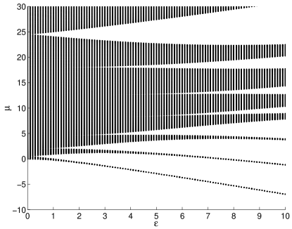
Figure 1: The bandgaps (unshaded areas) in the identical spectra of three linearized equations (13), with $\mu$ standing for any chemical potential, $\mu_{\phi}$, $\mu_{u}$, or $\tilde{\mu}_{v}$.

To conclude the description of the model, it is relevant to stress that the fluctuations, $u(x)$ and $v(x)$, must include contributions from all Bloch bands of the periodic potential. For sufficiently large $\varepsilon$, the lowest bands are narrow, hence the Bloch states in each of them may be approximated by a single mode in $u$ and $v$. For instance, inspection of the spectrum from Fig. 1 for $\varepsilon=5$ (this value will be used below) demonstrates that the three lowest bands are indeed sufficiently narrow to be approximated by single modes, while other bands have little relevance as they correspond to very high values of the chemical potential. Furthermore, in this situation contributions from mode-mixing cross terms to quadratic quantities (integrated densities, that measure the strength of the fluctuation components in the Bose gas, see below) are negligible, in view of the effective mutual incoherence of the Bloch wave functions in distinct narrow bands separated by wide gaps. Therefore, in such a representation, the integral quantities actually take the familiar form of diagonal sums over several fluctuation modes HFB -depletion-dark .

III Numerical results: families of partially incoherent gap solitons

III.1 Intragap solitons

Generic examples of solutions to Eqs. (13) with $T=0$ and $T>0$, in the form of intragap GSs with the three chemical potentials falling in the first or second bandgap, are shown in Fig. 2. In terms of Ref. Gubeskys , they are categorized as tightly and loosely bound solitons, respectively. Note that $\mathcal{N}_{B}=1$ corresponds to $T\approx 70$ nK, if the transverse trapping frequency is $2\pi\times 1~{}$KHz. In Fig. 2, it is seen that the soliton does not suffer drastic changes with the increase of temperature.

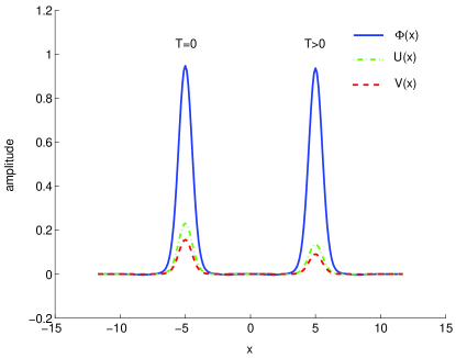
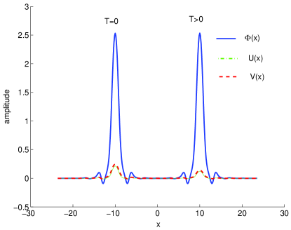
Figure 2: (Color online) Typical examples of stable intragap solitons found for $T=0$ and $T>0$, which correspond to Bose occupancy $\mathcal{N}_{B}=0$ and $1$, respectively [see Eq. (9)] in the first (a) and second (b) bandgaps, with (a) $\mu_{u}=-2$, $\tilde{\mu}_{v}=-2.5$, $\mu_{\phi}=-2.25$; (b) $\mu_{u}=1.5$, $\tilde{\mu}_{v}=3$, $\mu_{\phi}=2.25$. In this and other examples, the OL strength is $\varepsilon=5$.

Families of partially incoherent GSs can be characterized by fractions of the vapor components in the total number of atoms, i.e., $N_{u}/N$ and $N_{v}/N$ [see Eq. (10)], as functions of $\mu_{u}$ and $\tilde{\mu}_{v}$, each chemical potential varying within a given bandgap. In Fig. 3 we display these dependences for $T=0$, with both $\mu_{u}$ and $\tilde{\mu}_{v}$ belonging to the first or second bandgap [then $\mu_{\phi}=\left(\mu_{u}+\tilde{\mu}_{v}\right)/2$, see Eq. (12), lies in the same gap, hence the families are of the intragap type, indeed]. A “valley” in the plots running along the diagonal means that the symmetric solutions, with $\mu_{u}=\tilde{\mu}_{v}$, amount to the ordinary GSs, with $u=v=0$. All solitons belonging to these families in the first and second gaps feature, respectively, tightly- and loosely-bound shapes, similar to those in Fig. 2.

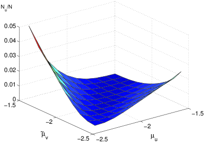
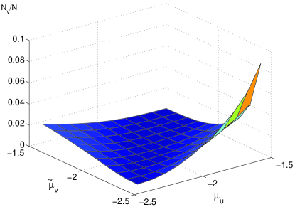
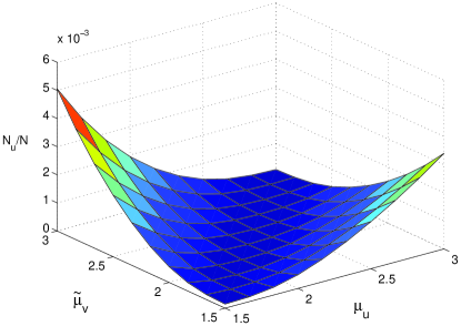
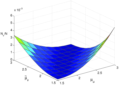
Figure 3: (Color online) The vapor fractions $N_{u}/N$ and $N_{v}/N$ in families of stable tightly and loosely bound intragap solitons in the first (a,b) and second (c,d) bandgaps versus $\mu_{u}$ and $\tilde{\mu}_{v}$, at $T=0$.

Figure 4 shows that the dependence of $N_{u}/N$ and $N_{v}/N$ on temperature is very weak, at fixed values of $\mu_{u}$ and $\tilde{\mu}_{v}$ (in the temperature range considered). Counterparts of the latter dependence for fixed $N$ (rather than fixed chemical potentials) may be interesting too, but they need a large pool of numerical data and will be reported elsewhere.

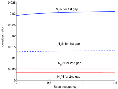
Figure 4: (Color online) The vapor fractions $N_{u}/N$ and $N_{v}/N$ vs. temperature [shown via Bose occupancy $\mathcal{N}_{B}$, see Eq. (9)] for the same solitons as in Fig. 2.

III.2 Intergap and higher-order solitons

A family of intergap solitons has been constructed too, with the chemical potentials of the fluctuational components, $\mu_{u}$ and $\tilde{\mu}_{v}$, belonging to the first and second bandgaps, respectively [then, the condensate’s chemical potential, locked to $\mu_{u}$ and $\tilde{\mu}_{v}$ as per Eq. (12), $\mu_{\phi}=\left(\mu_{u}+\tilde{\mu}_{v}\right)/2$, belongs to the second bandgap too]. A typical soliton of this type is shown in Fig. 5. Note that its $U(x)$ component, which corresponds to the chemical potential, $\mu_{u}$, which belongs to the first bandgap, features a typical tightly bound shape, cf. Fig. 2(a), while the shapes of the other two components, $\Phi(x)$ and $V(x)$, which pertain to the chemical potentials, $\mu_{\phi}$ and $\tilde{\mu}_{v}$, which belong to the second bandgap, are weakly bound, cf. Fig. 2(a).

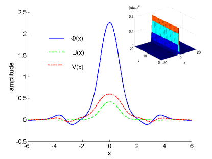
Figure 5: (Color online) An intergap soliton at $T=0$, with chemical potentials $\mu_{u}=0$ and $\tilde{\mu}_{v}=3$, $\mu_{\phi}=1.5$, which fall in the first and second bandgaps, respectively. The inset illustrates stability of the perturbed intergap soliton in direct simulations.

The $N_{u}/N$ and $N_{u}/N$ characteristics for the entire intergap family are presented in Fig. 6. Note that intergap solitons with $u=v=0$ do not exist, unlike their intragap counterparts, therefore these plots do not feature “valleys”, unlike Fig. 3.

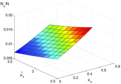
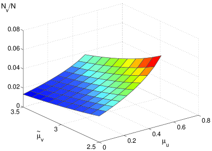
Figure 6: (Color online) The vapor fractions $N_{u}/N$ and $N_{v}/N$ in the family of intergap solitons, at $T=0$, versus chemical potentials of the two fluctuational components, $\mu_{u}$ and $\tilde{\mu}_{v}$, belonging to the first and second bandgaps, respectively.

In addition to the fundamental (single-humped) GSs, various types of higher-order multi-humped states have been found too. In Fig. 7, we display (for $T=0$ and $T>0$) the simplest among them, which is single-humped in the condensate field ($\phi$), and doubled-humped in one of the vapor components.

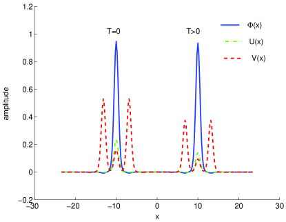
Figure 7: Stable higher-order solitons in the first bandgap, for the same parameters as in Fig. 2(a).

Obviously, the higher-order soliton shown in Fig. 7 is not a bound state of fundamental solitons. On the other hand, straightforward bound states can be found too, see an example of a three-soliton complex in Fig. 8. Note that, as per a general principle for the stability of bound solitons on lattices Todd , this complex may be stable because the phase difference between the bound solitons is $\pi$.

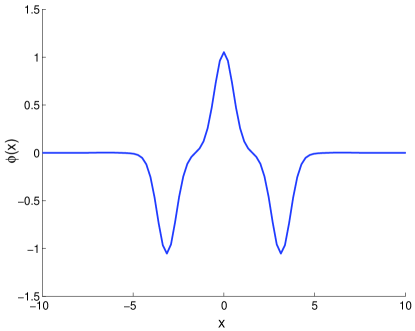
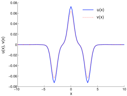
Figure 8: (Color online) An example of a stable bound state of three fundamental solitons belonging to the first bandgap (for $\mu_{u}=-2.0$, $\tilde{\mu}_{v}=-2.2$, $\mu_{\phi}=-2.1$): the condensate component (a) and vapor wave functions (b).

As well as the fundamental intra- and intergap solitons, their higher-order counterparts of various types form families which fill out the bandgaps.

IV Stability analysis

The stability of the GSs was first tested in direct simulations, which has demonstrated that they are all appear to be stable, both at $T=0$ and $T>0$. Most accurate information about the stability can be obtained from computation of eigenvalues for small perturbations, using equations (1) and (8) linearized around stationary solitons. In particular, the stability of ordinary GSs was previously shown in the framework of the Bogoliubov–de Gennes equations, which are derived by the linearization of the GP equation about the solitons Markus .

Following this approach, we first consider the stability of the GSs with $u=v=0$ (i.e., the subfamily along the diagonal “valleys” in Fig. 3) against small vapor perturbations, $u=e^{-i\lambda t}u_{1}(x)$ and $v=e^{i\left(2\mu_{\phi}-\lambda\right)t}v_{1}(x)$, where $\lambda$ is the perturbation eigenvalue. The instability implies the existence of eigenvalues with $\mathrm{Im}(\lambda)>0$. In this case, linearized equations (8) decouple from Eq. (1), yielding

$$(1/2)u_{1}^{\prime\prime}+\left[\varepsilon\cos(2x)-2\rho\left|\Phi\right|^{2}\right]u_{1}+\Phi^{2}v_{1} = \lambda u_{1},$$

$$(1/2)v_{1}^{\prime\prime}+\left[\varepsilon\cos(2x)-2\rho\left|\Phi\right|^{2}\right]v_{1}+\Phi^{2}u_{1} = -\left(2\mu_{\phi}+\lambda\right)v_{1}.$$ (14)

Solving these equations (which do not depend on temperature) numerically (with proper boundary conditions), we have concluded that all GSs with zero vapor components are stable against “vaporization”.

Then, we performed the linear-stability analysis for the full GSs, including nonzero vapor components. We have found that the families of intragap solitons in both (first and second) bandgaps are completely stable (for $T=0$ and $T>0$ alike), in complete accordance with direct simulations. Preliminary considerations of higher-order intragap solitons, such as ones displayed in Figs. 7 and 8, suggest that they are stable too.

For the intergap family, a weak instability is revealed by the computation of eigenvalues, see Fig. 9 (since intergap solitons cannot exist without vapor components, this instability is specific to the partially incoherent GSs). However, this weak instability does not manifest itself in direct simulations (as shown, for instance, by inset in Fig. 5), which suggests that the intergap solitons, even though being formally unstable, may be observed in experiments.

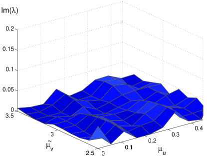
Figure 9: The instability growth rate for the family of intergap solitons (at $T=0$), as found from numerical solution of the linearized equations for small perturbations.

It is also relevant to check the stability of the solitons against deviations from the one-dimensionality Luca . In the simplest approximation, this amounts to modifying the equations, keeping them effectively one-dimensional but adding quintic terms to the cubic nonlinearity friction ; Lev . Preliminary analysis shows that no additional instability emerges in this way.

V Conclusion

We have found families of matter-wave gap solitons (GSs) in the degenerate Bose gas with repulsive interactions between atoms, trapped at zero or finite temperature in a periodic optical-lattice (OL) potential. Stability of the GSs was studied too. The solitons include a coherent condensate wave function, and two components of the incoherent “vapor” (which actually comprise many fluctuation modes, due to the OL’s band structure). Chemical potentials of all constituents of the GS must fall in bandgaps. Accordingly, families of intra- and intergap solitons (including higher-order ones, and bound states of fundamental solitons) were found in the two lowest bandgaps, and it was concluded that they do not change drastically with the growth of temperature. While the intragap GSs are completely stable, their counterparts of the intergap type feature a very small unstable perturbation eigenvalue, but, nevertheless, they do not feature any tangible instability in direct simulations.

We acknowledge valuable discussions with A. Vardi. This work was supported in part by Israel Science Foundation (Center-of-Excellence grant No. 8006/03) and U.S.-Israel Binational Science Foundation (grant No. 2002147).

References

- (1) A. Griffin, Phys. Rev. B 53, 9341 (1996); N. P. Proukakis and K. Burnett, J. Res. Natl. Inst. Stand. Technol. 101, 457 (1996); N. P. Proukakis, K. Burnett, and H. T. C. Stoof, Phys. Rev. A57, 1230 (1998); P. O. Fedichev and G. V. Shlyapnikov, Phys. Rev. A58, 3146 (1998); M. Holland, J. Park, and R. Walser, Phys. Rev. Lett. 86, 1915 (2001); A. M. Rey, B. L. Hu, E. Calzetta, A. Roura, and C. W. Clark, Phys. Rev. A69, 033610 (2004).
- (2) H. Buljan, M. Segev and A. Vardi, Phys. Rev. Lett. 95, 180401 (2005).
- (3) M. Lewenstein and L. You, Phys. Rev. Lett. 77, 3489 (1996); Y. Castin and R. Dum, ibid. 79, 3553 (1997).
- (4) J. Dziarmaga, Z. P. Karkuszewski, and K. Sacha, Phys. Rev. A 66, 043615 (2002); J. Dziarmaga and K. Sacha, ibid. 66, 043620 (2002); C. K. Law, ibid. 68, 015602 (2003); A. E. Muryshev, G. V. Shlyapnikov, W. Ertmer, K. Sengstock, and M. Lewenstein, Phys. Rev. Lett. 89, 110401 (2002).
- (5) R.-K. Lee , E. A. Ostrovskaya, Y. S. Kivshar, and Y. Lai, Phys. Rev. A 72, 033607 (2005).
- (6) L. Salasnich, J. Phys. B – At. Mol. Opt. Phys.39, 1743 (2006).
- (7) S. Sinha , A. Yu. Cherny, D. Kovrizhin, and J. Brand , Phys. Rev. Lett. 96, 030406 (2006).
- (8) L. Khaykovich, F. Schreck, G. Ferrari, T. Bourdel, J. Cubizolles, L. D. Carr, Y. Castin, and C. Salomon, Science 296, 1290 (2002); K. E. Strecker, G. B. Partridge, A. G. Truscott, and R. G. Hulet, Nature 417, 150 (2002).
- (9) S. L. Cornish, S. T. Thompson, and C. E. Wieman, Phys. Rev. Lett. 96, 170401 (2006).
- (10) M. Mitchell, Z. Chen, M. Shih, and M. Segev , Phys. Rev. Lett. 77, 490 (1996); M. Mitchell , M. Segev, T. H. Coskun and D. N. Christodoulides , Phys. Rev. Lett. 79, 4990 (1997); M. Mitchell and M. Segev, Nature 387, 880 (1997); D. N. Christodoulides , E. D. Eugenieva, T. H. Coskun, M. Segev, M. Mitchell , Phys. Rev. E 63, 035601(R) (2001).
- (11) A. Trombettoni and A. Smerzi, Phys. Rev. Lett. 86, 2353 (2001); F. Kh. Abdullaev , B. B. Baizakov, S. A. Darmanyan, V. V. Konotop and M. Salerno, , Phys. Rev. A 64, 043606 (2001); I. Carusotto, D. Embriaco, and G. C. La Rocca, ibid. 65, 053611 (2002); B. B. Baizakov, V. V. Konotop, and M. Salerno, J. Phys. B35, 5105 (2002); E. A. Ostrovskaya and Y. S. Kivshar, Phys. Rev. Lett. 90, 160407 (2003).
- (12) B. Eiermann et al., Phys. Rev. Lett. 92, 230401 (2004).
- (13) V. Ahufinger and A. Sanpera, Phys. Rev. Lett. 94, 130403 (2005).
- (14) A. Gubeskys, B. A. Malomed, and I. M. Merhasin, Phys. Rev. A73, 023607 (2006).
- (15) O. Cohen, T. Schwartz, J. W. Fleischer, M. Segev, and D. N. Christodoulides, Phys. Rev. Lett. 91, 113901 (2003).
- (16) A. A. Sukhorukov and Y. S. Kivshar, Phys. Rev. Lett. 91, 113902 (2003).
- (17) V. M. Pérez-García, H. Michinel, and H. Herrero, Phys. Rev. A 57, 3837 (1998); L. Salasnich, A. Parola, and L. Reatto, Phys. Rev. A 65, 043614 (2002); A. E. Muryshev, G. V. Shlyapnikov, W. Ertmer, K. Sengstock, and M. Lewenstein, Phys. Rev. Lett. 89, 110401 (2002); Y. B. Band, I. Towers, and B. A. Malomed, Phys. Rev. A 67, 023602 (2003); S. Sinha, A. Y. Cherny, D. Kovrizhin, and J. Brand, Phys. Rev. Lett. 96, 030406 (2006).
- (18) L. Khaykovich and B. A. Malomed, Phys. Rev. A, in press (article No. AS10005).
- (19) T. Kapitula, P. G. Kevrekidis, and B. A. Malomed,. Phys. Rev. E 63, 036604.
- (20) K. M. Hilligsøe, M. K. Oberthaler, K. P. Marzlin, Phys. Rev. A66, 063605 (2002); D. E. Pelinovsky, A. A. Sukhorukov, and Y. S. Kivshar, Phys. Rev. E 70, 036618 (2004).