Influence of Temperature Gradients on Tunnel Junction Thermometry below 1 K: Cooling and Electron-Phonon Coupling

Abstract

We have studied thermal gradients in thin Cu and AlMn wires, both experimentally and theoretically. In the experiments, the wires were Joule heated non-uniformly at sub-Kelvin temperatures, and the resulting temperature gradients were measured using normal metal-insulator-superconducting tunnel junctions. The data clearly shows that even in reasonably well conducting thin wires with a short ($\sim 10$ $\mu$m) non-heated portion, significant temperature differences can form. In most cases, the measurements agree well with a model which includes electron-phonon interaction and electronic thermal conductivity by the Wiedemann-Franz law.

PACS numbers: 73.23.-b, 72.10.Di, 74.50.+r

1 INTRODUCTION

Temperature is naturally the most critical quantity in studies of any thermal properties of materials, and its measurement is typically a non-trivial task. In nano- and mesoscopic structures at low temperatures, this task is made even harder by the small size of the samples and their sensitivity to any external noise power, which is caused by weakness of the electron-phonon interaction.[1] Because of this weakness, electrons can be easily overheated (or cooled) with respect to phonons at temperatures below 1K, a phenomenon known as the hot-electron effect.[2] In this quasiequilibrium regime, valid in many situations, the electronic and phononic degrees of freedom attain their own internal equilibrium temperatures, with a power flowing between them. Given this regime, it is possible to measure the electron temperature, if a suitable thermometer is found.

A good choice for electron thermometry below 1K is normal metal-insulator-superconductor (NIS) tunnel junction thermometers,[3, 4] known for their sensitivity. They can also be fabricated to a very small size $\sim 100\times 100$ nm, so that it is possible to measure local temperatures. However, there are few studies describing how sample geometry affects temperature profiles in mesoscopic samples, and consequently how it complicates the interpretation of temperature measurements.

In this paper, we discuss experimental and theoretical results on temperature gradients in mesoscopic metal wires with non-uniform Joule heating. The experiments were performed with NIS junctions, therefore allowing us to measure temperatures at several locations. We observe that there are significant temperature gradients in copper and aluminum manganese wires, even if the non-heated portion of the wire is only $\sim 10$ $\mu$m long. The experimental observations can be explained successfully by numerical solution of a non-linear differential equation describing the heat balance, which incorporates the Wiedemann-Franz law and electron-phonon coupling theory. In addition, we also present numerical results on temperature profiles caused by non-uniform cooling, modeling e.g. tunnel junction coolers.[4]

The paper is organized as follows: Sec. 2 discusses the theory. In Subs. 2.1 we briefly review the theory of electron-phonon interaction in disordered films, followed by the numerical results on non-uniform Joule heating in 2.2 and on cooling in 2.3. Section 3 presents the experimental techniques, with the experimental results presented in Sec. 4. Conclusions are drawn in Sec. 5. —

2 THEORY AND NUMERICAL RESULTS

2.1 Electron-phonon coupling in metals

Electron-phonon (e-p) scattering is a critical process for understanding how electron gas relaxes energy. It is the dominant mechanism for electron energy loss below 1 K, as photon radiative losses are very small except in the smallest samples.[5, 6] The strength of e-p coupling depends significantly on several factors: the material in question; the level of disorder in the metal, parametrized by the electron mean free path $l$;[7, 8] and the type of scattering potential.[9]

In general, the electron-phonon scattering rate has a form

$$\frac{1}{\tau_{e-p}}=\alpha T_{e}^{m},$$ (1)

and the corresponding net power density transferred from hot electrons to phonons is

$$p=\Sigma(T_{e}^{n}-T_{p}^{n}),$$ (2)

where $\Sigma$ describes the strength of electron-phonon coupling, $T_{e}$ is the electron and $T_{p}$ the phonon temperature, and $n=m+2$. The exact form of coupling constant $\Sigma$ and the exponent $n$ is determined by the disorder, mainly depending on the parameter $ql$, where $q$ is the wavevector of the dominant thermal phonons.

In ordered metals, defined as $ql>1$, electrons can scatter either from longitudinal only, or from longitudinal and transverse phonons depending on temperature and material.[10] When scattering happens only from longitudinal phonons, the temperature dependence for scattering rate $\tau_{e-p}^{-1}$ is $m=3$ and, for the heat flow in Eq. (2), $n=5$.[1, 11] In this case, the coupling constant $\Sigma$ is only a material dependent parameter. If electrons interact dominantly with transverse phonons, $m=2$, $n=4$ and $\Sigma\propto 1/l$.[9] However, if the scattering rates for transverse and longitudinal phonons are are of the same magnitude, $m$ can vary continuously between $m=2-3$, so that $n=4-5$ and $\Sigma\propto l^{-1}-l^{0}$. [9]

In disordered metals, where $ql<1$, electrons scatter strongly from impurities, defects and boundaries, and the situation is more complicated to model because of the interference processes between pure electron-phonon and electron-impurity scattering events. However, there is a theory that includes electron-impurity scattering by vibrating and static disorder.[9] In the case of fully vibrating impurities (following the phonon mode) $m=4$, $n=6$ and $\Sigma\propto l$. On the other hand, if the scattering potential is completely static, electrons interact only with longitudinal phonons and at low temperatures $m=2$, $n=4$ and $\Sigma\propto 1/l$. Between these two extremes there is a region, where the scattering potential is a mixture of the two, and theory predicts exponents $m$ ranging between 2-4 and $\Sigma$ depending on $l$ as $l^{k}$, where $k$ ranges between -1 and 1.

2.2 Numerical results on Joule heating

Non-uniform heating and/or cooling profiles generate temperature gradients, even in good conductors such as copper. The magnitude of the effect is determined by the ratio of the energy flow due to electronic diffusion (thermal conductance) to that of the energy flow to the phonons. If diffusive flow is much larger, small temperature gradients exist and vice versa. Therefore, it is intuitively clear that more resistive samples have larger gradients, if the electron-phonon interaction does not depend on the mean free path $l$. However, as we discussed in the previous section, in impure metal films the strength of the e-p interaction does actually depend on $l$, and a priori it is not fully clear how this affects the temperature profiles.

To study the temperature profiles in mesoscopic metallic samples, we need to solve numerically the non-linear differential equation describing the heat flow in the system. We restrict ourselves to the simplest one-dimensional problem, which is valid for wires of approximately constant cross section. This is a good approximation for the samples described in the next section (Table 1). The heat equation for a sample with uniform resistivity $\rho$ reads

$$\frac{d}{dx}\left(\frac{{\cal L}}{\rho}T(x)\frac{dT(x)}{dx}\right)=\Sigma[T(x)^{n}-T_{p}^{n}]-\dot{q}_{h}(x)+\dot{q}_{c}(x),$$ (3)

where we have used the Wiedemann-Franz law for electronic thermal conductivity $\kappa={\cal L}T/\rho$ with ${\cal L}=\pi^{2}k_{B}^{2}/(3e^{2})$ the Lorentz number,[12] and where $\dot{q}_{h}(x)$ and $\dot{q}_{c}(x)$ are the power density profiles for heating and cooling, respectively. If one heats the wire with a dc current density $i$, the Joule heating power density will be given by $\dot{q}_{h}(x)=\rho i^{2}f(x)$, where $f(x)=1$ at points where current flows, and $f(x)=0$ elsewhere. Typically, this problem has been solved for Dirichlet boundary conditions, for which temperature is fixed at the boundary. The Dirichlet problem describes well the case in which the wire is in direct contact with thick and wide normal electrodes,[13] whose temperature stays constant. In contrast, our sample geometry is such that the wire does not have any contacts at the physical ends, and the heating current is passed through superconducting leads in direct contact with the wire (NS boundaries), so that no heat flow takes place through them. In this case, the correct boundary conditions are the von Neumann type, where $dT/dx=0$.

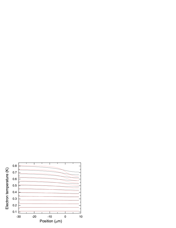
Figure 1: Color online. Calculated temperature profiles with varying Joule power levels applied uniformly at positions $x<0$. Solid (black) line uses material parameters for Cu sample 2 and dashed (red) line for the AlMn sample, see Tables 1 and 2. $T_{p}=60$ mK.

First, we discuss the numerical results on Joule heated wires. In this case the heated portion of the wire is much longer than the typical electron-electron scattering length at sub-Kelvin temperatures ($L\sim 0.5$ mm $>>L_{e-e}\sim 1$ $\mu$m), and therefore quasiequilibrium with a well defined electron temperature exists everywhere in the wire. In addition to the heated part of the wire, a short stub of length $d=9$ $\mu$m (corresponding to Cu sample 2, see Table 1) extends beyond the heated portion, where electrons can only diffuse and be cooled by phonons. This means that the temperature will start to fall, and the magnitude of this drop is a strong function of temperature itself. The first (and wrong, as we will see) intuition is that if the stub is much shorter than the length scale for phononic energy relaxation $L_{e-p}=\sqrt{D\tau_{e-p}}$, where $D$ is the diffusion constant, there is no significant effect below 1 K, as $L_{e-p}$ ranges between $\sim$1 mm and 10 $\mu$m at 100 mK - 1 K for typical thin films.

Figure 1 shows the calculated temperature profiles for different Joule powers using the materials parameters for our experimental sample Cu 2 (solid) and the AlMn sample (dashed) (Tables 1 and 2). The phonon temperature $T_{p}$ was set to 60 mK, which is the refrigerator temperature used in the experiments. The length of the stub was kept constant, using the value for the Cu 2 sample $d=9$ $\mu$m. The x-coordinate is such that Joule power is applied at $x<0$, and the Joule power levels between Cu and AlMn are adjusted so that the electron temperatures in the bulk of the wires are equal. It is very clear that a short stub of this length does, in fact, have a significant effect on the profiles, contrary to our initial expectation. At $T>300$ mK, the temperature drop seems to be measurable for both materials, and stronger for AlMn, which has approximately five times higher resistivity, but also a weaker e-p scattering rate. Interestingly, the temperature drop extends mostly into the area $x<0$, where Joule heat is being uniformly applied. Therefore, the bulk electron temperature, determined solely by the electron-phonon scattering, can only be measured at $>40$ $\mu$m distance away from the end of the wire. In the next section we describe the experiments used to study these temperature gradients.

In Fig. 2, we also plot the same profiles scaled to the bulk values for each Joule power, so that the full temperature profile is clearly seen for all temperatures. We see that the length scale for the temperature drop grows strongly to $>100$ $\mu$m as one lowers the bulk temperature to 100 mK (top curve), although the relative drop becomes small. Also, the temperature profile is highly non-symmetric with respect to the average temperature, as expected for a non-linear system. At the higher temperature range, the AlMn profiles become clearly steeper due to the differences in $\rho$, $\Sigma$ and $n$.

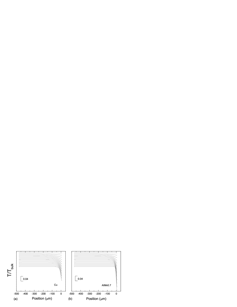
Figure 2: Calculated relative temperature profiles $T/T_{bulk}$ with varying Joule power levels applied at positions $x<0$. Parameters used are the same as in Fig. 1, (a) Cu sample 2, and (b) AlMn sample. Note that the curves have been shifted for clarity. Top curve corresponds to the lowest temperature $T_{bulk}\approx 100$ mK.

From the calculated profiles, one can see how the length scale and magnitude of the temperature drop depend on the bulk wire temperature. This is shown in Fig. 3. We have defined the energy loss length as the distance where $T$ changes 90 % of the total change measured from the end of the stub. By comparing with the theoretical electron-phonon length $L_{e-p}$ in Fig. 3 (a), we see that our definition corresponds to roughly $\sim 2.2L_{e-p}$, with the correct temperature dependence determined by the e-p scattering $L_{e-p}\sim T^{m/2}$, where $m=3$ for Cu and $m=4$ for AlMn (Table 2). The deviations at low temperatures are due to saturation caused by $2L_{e-p}$ approaching the length of the wire. The high temperature deviation in the case of AlMn shows that, at higher Joule power levels, the energy loss length is not simply given by $\sim 2L_{e-p}$. We do not have a theoretical description for the magnitude of the temperature drop, which must be a function of the stub length $d$. However, we have simply plotted the values in Fig. 3 (b) with the observation that they follow a power law of the form $\Delta T\sim T^{(m+2)/2}$ for both materials, where $(m+2)$ and 2 are the exponents of the temperature dependencies of the heat flow rates due to e-p interaction and diffusion, respectively.

Figure 3: (a) Symbols: Calculated energy loss length, defined as the length where $T$ has changed 90 % of the total change. Squares: Cu, Triangles: AlMn. Solid lines show theoretical values $2.2L_{e-p}$. Dashed lines shows the length of the wire. (b) Magnitude of the temperature drop, Squares: Cu, Triangles: AlMn. Solid lines are fits to power laws. Parameters used are the same as in Fig. 1.

2.3 Numerical results on NIS tunnel junction cooling

So far we considered the case in which we had a non-uniform Joule heating profile. Technologically important is also the case in which a non-uniform cooling profile exists. This is in practice the case always for normal metal-insulator superconductor (NIS) tunnel junction electron coolers,[4] as they never cover the whole area of the normal metal being cooled (there has to be room for thermometers). However, if the total dimensions of the normal metal island are small compared to $L_{e-p}$ (regardless of how much area is uncooled), no significant gradients will develop. On the other hand, especially difficult is the case of phonon membrane coolers,[14, 15] where the cooler junctions are located on the bulk of the wafer and extend a normal metal cold finger onto a thin insulating membrane. In that case, temperature gradients have to be taken into account.

In Fig. 4 we plot the calculated temperature profiles for a long wire with a uniform cooling power applied at positions $x>0$ and for a constant phonon temperature $T_{p}=340$ mK, with Cu sample 2 and AlMn sample parameters (Tables 1, 2). The cooling power was chosen so that the minimum temperature would reach $\sim$ 100 mK, which is a typical value for aluminum based tunnel junction coolers. [4] It is clear that the temperature starts to rise already within the cooled area, and rises back to the bulk value of $T_{p}$ within approximately $100$ $\mu$m, given by $\sim 2L_{e-p}$ as before. This shows that effective cooling only works some tens of microns away from the junctions on the bulk substrate. When modeling membrane coolers more accurately, it is necessary to take into account the gradients of the phonon temperature [16] and the fact that the electron-phonon interaction strength is weakened on membranes.

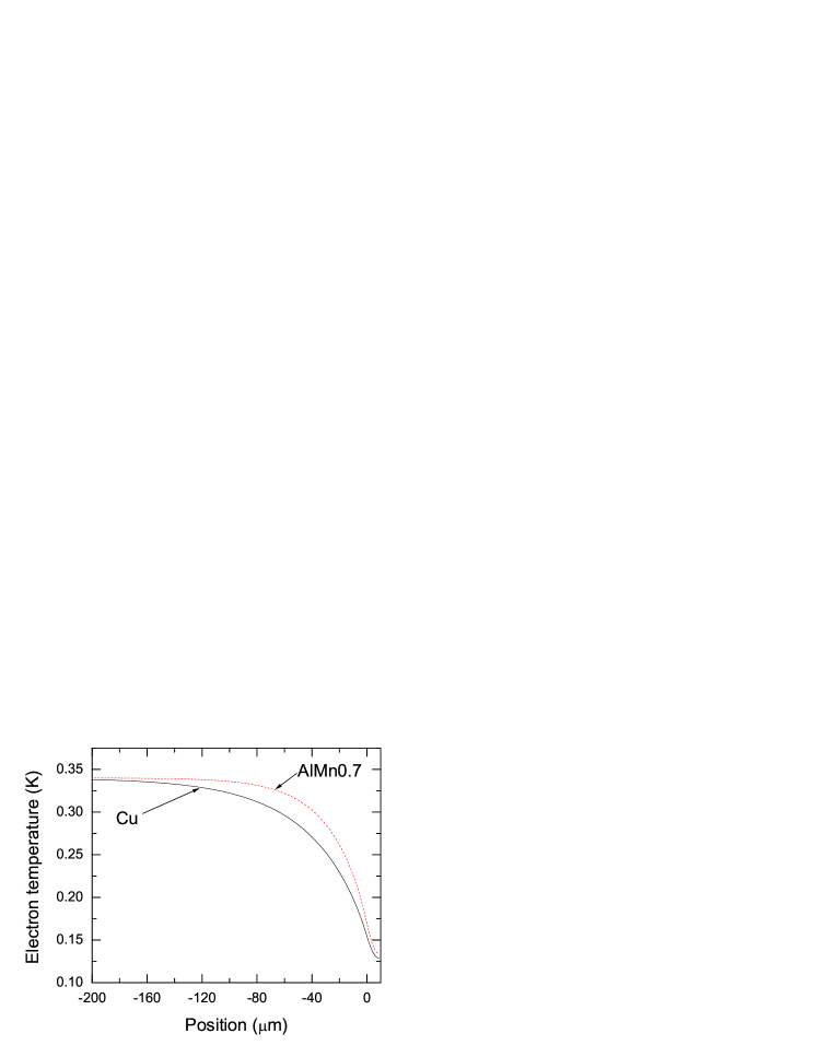
Figure 4: Color online. Calculated temperature profiles with a cooling power applied at positions $x>0$. Solid (black) is the result for Cu sample 2 and (red) dashed line for the AlMn sample. Parameters used are the same as in Fig. 1.

—

3 EXPERIMENTAL TECHNIQUES AND SAMPLES

We performed non-uniform heating experiments on several Cu and AlMn wires. All samples were fabricated on oxidized or nitridized silicon chips by standard e-beam lithography and multi-angle shadow mask evaporation techniques. Figure 5 shows the schematic picture of the samples and the measurement circuit. Table 1 presents the essential dimensions of the samples measured by SEM and AFM. The resistivity $\rho$ was determined from the I-V measurement of the wire at 60 mK, from which the mean free path $l$ was calculated using the Drude formula.

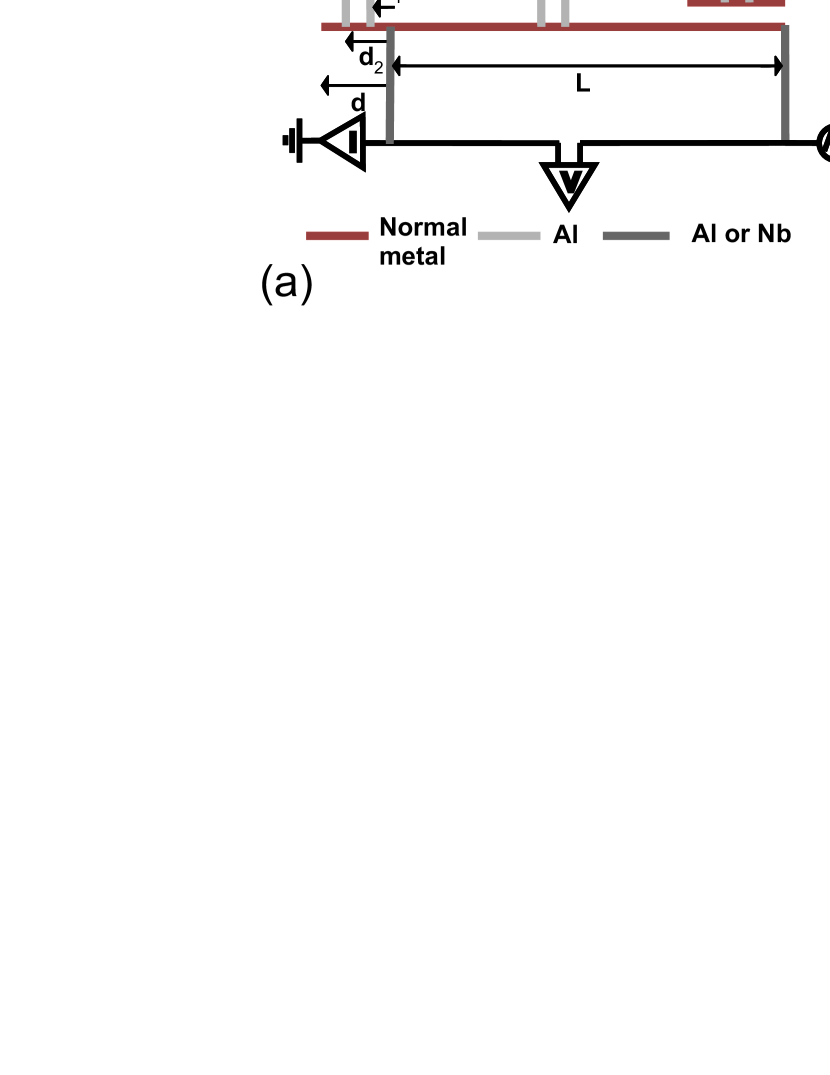
Figure 5: (a) Schematic of the sample geometry and the measurement circuit. Black lines are the normal metal (Cu or AlMn), dark gray Al, and light gray Al or Nb. All the Al leads above the normal metal wire form NIS tunnel junctions, whereas the Al or Nb leads below have direct NS contacts. $L$ is the length of the heated part of the wire and $d$ is the length of the unheated part. $d_{1}$ and $d_{2}$ are the positions of the NIS-junctions from the nearest NS-interface. (b) An SEM picture of an SN interface and a SINIS junction at the end of the heated wire of a representative sample.

All samples have a normal metal wire of length $\sim$ 500 $\mu$m and width $\sim$ 400-600 nm, onto which two Al (Nb for Cu sample 2) leads form direct normal metal-superconductor (NS) interfaces. In addition, two pairs of Cu-AlO_x-Al (NIS) tunnel junctions connect to the wire. The NS contacts are used to pass the heating current, and the SINIS junctions serve as electron thermometers in the middle and at the end of the wire. Near the heated wire, there is also a short, electrically isolated normal metal wire with a SINIS thermometer, which measures the local phonon temperature.

Table 1: Parameters of measured Cu and AlMn samples. $L$, $d$, $d_{1}$ and $d_{2}$ are defined in Fig. 5, $t$ is the thickness and $A$ the cross sectional area of the normal metal wire. $\rho$ is the measured resistivity, and $l$ the mean free path.

Parameter	Cu sample 1	Cu sample 2	Cu sample 3	AlMn sample
$L$ [$\mu$m]	473	473	492	466
$d$ [$\mu$m]	11	9	20	16
$d_{1}$ [$\mu$m]	3	2	7	7
$d_{2}$ [$\mu$m]	8	8	14	10
$t$ [nm]	48	32	28	55
$A$ [x10-14m2]	1.5	1.5	2.5	1.4
$\rho$ [x10${}^{-8}\Omega$m]	2.5	3.0	3.8	12.3
$l$ [nm]	27	22	17	3.2

Because of Andreev reflection at the NS-junctions, which are biased within the superconducting gap $\Delta$, the Joule heating current in the normal metal is converted into a supercurrent in the superconductor, which does not carry any heat with it. Thus, the NS contacts are very good electrical conductors and, in the ideal case, perfect thermal insulators. This way the Joule heat does not leak into the superconducting side and the NS contacts do not cause any thermal gradients. In other words, the Joule heat is uniform between the the NS contacts. While the Joule current is being applied, we can simultaneously measure the applied power $P$ from the measurement of current and voltage in four probe configuration, the electron temperature in the middle of the wire, where no gradients exist, as well as at the end of the wire, where significantly lower temperatures are expected. More details of the typical thermometer biasing and calibration are described in Ref. 17. The effect of the thermometers on the temperature profile was estimated to be insignificant.

—

4 EXPERIMENTAL RESULTS

As the thermometer approximately in the middle of the wire (the middle thermometer) measures the temperature in a region without thermal gradients (Sec. 2.2), we see that Eq. (3) will reduce to $\dot{q}_{h}=\Sigma(T_{e}^{n}-T_{p}^{n})$, and the values of $n$ and $\Sigma$ can be determined from the data. The thermometer at the unheated end of the wire (the side thermometer), on the other hand, lies in the region of a gradient. As it comprises of two NIS-tunnel junctions separated by a small, but a significant distance, the two junctions measure two different temperatures, and the combined SINIS measurement will give a value in between these two temperatures. The measured temperature is not necessarily the average of the two due to the nonlinearity of the NIS thermometer.

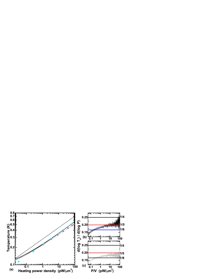
Figure 6: Color online. Data from Cu sample 1. (a) The temperatures of the thermometers vs heating power density in log-log scale. Black line: experimental data from the middle thermometer. Gray line: experimental data from the side thermometer. Gray (Cyan) circles: numerical results for the middle thermometer, and gray (pink) stars: numerical results for the side thermometer. Dashed line is a guide to the eye $T\propto$ $(P/V)^{1/5}$. (b) The logarithmic numerical derivatives of the experimental middle thermometer data, and (c) the same for the side thermometer.

Cu samples 1 and 2 have a similar sample geometry, except for a difference in the thickness $t$, and in the electron mean free path $l$. In Fig.s 6(a) and 7(a) we plot the temperatures of both thermometers vs heating power density $P/V$ in log-log scale. Clear temperature difference between the two thermometers can be seen at $P/V>1$ pW/$\mu$m³, and at 100 pW/$\mu$m³ the difference is roughly 50 mK. Below 0.1 pW/$\mu$m³ both temperatures saturate mostly because of noise heating. The theoretical points have been calculated by solving Eq. (3) using the appropriate sample parameters. In the calculation, we used values for $\Sigma$ obtained from the middle thermometer data (Table 2). The temperature of the side SINIS thermometer is defined in our analysis as the average of the two NIS-junction temperatures. This definition is justified, because the difference between the two temperatures is small and within the size of the plotted datapoints for all sample geometries studied in this paper. From Figs.s 6(a) and 7(a) it is clear that the theory agrees well with the experimental data, showing that the observed temperature difference is fully explained by phonon cooling and diffusion.

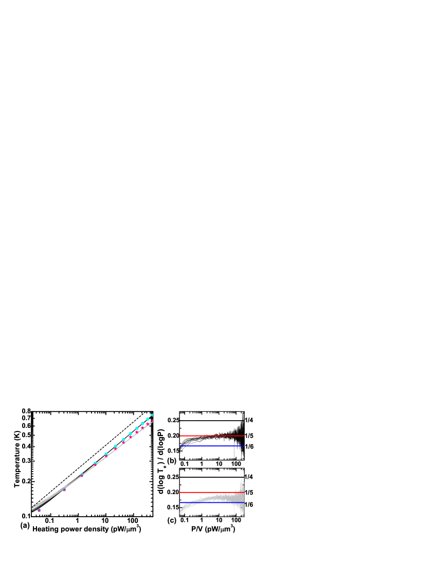
Figure 7: Data from Cu sample 2. Symbols are explained in the caption of 6.

From the phonon thermometer data (not shown), we have seen that $T_{e}\gg T_{p}$ for all samples in this work, and therefore for the middle thermometer we can approximate $P_{heat}/V=\Sigma T_{e}^{n}$, where $V$ is the volume of the heated portion of the wire. The temperature dependence $n$ and strength $\Sigma$ of electron-phonon interaction can thus be obtained from the plots of the middle thermometer temperature versus heating power density in s 6(a) and 7(a). A more detailed look at $n$ can be obtained by plotting the logarithmic derivatives $d(\log T_{e})/d(\log P)=1/n$, shown in Figs.s 6(b) and 7(b). Measured data in both samples scales clearly as $P\propto T_{e}^{5}$. However, because of the temperature drop at the end of the wire, the data from the side thermometer, Figs. 6(c) and 7(c), show a temperature dependence $P\propto T_{e}^{5.5}$. This exponent does not correspond to the actual power law of the e-p interaction.

Copper sample 3 is a bit thinner and has a longer unheated end section compared to samples 1 and 2 (Table 1). From Fig. 8(a) we observe that the measured temperature difference between the two thermometers is much larger than for samples 1 and 2, and also larger than what the theoretical calculation predicts. We do not fully understand this at the moment, but it is possible that the Lorentz number is reduced due to inelastic scattering on the surface.[12] Indeed, high resolution SEM images of sample 3 showed that the surface was more irregular. Nevertheless, we can obtain the temperature dependence of e-p interaction from the middle thermometer [Figs. 8(a), (b)], showing again an agreement with $P\propto T_{e}^{5}$, while the data from the side thermometer fits $P\propto T_{e}^{7}$.

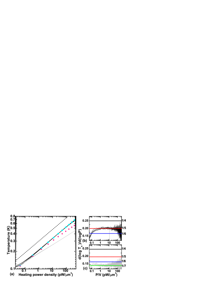
Figure 8: Data from Cu sample 3. Symbols are explained in the caption of Fig. 6.

The last sample is made from aluminum doped with 0.7 at % manganese. Due to the high impurity concentration, the mean free path $l$ is much shorter than for copper wires, and the AlMn wire is $\sim$ 4 times more resistive (Table 1). Figure 9(a) shows that the measured data and the numerical result agree well. It may be surprising, perhaps, that the temperature difference between the thermometers is actually smaller than in Cu sample 3. Although the AlMn sample is more resistive and thus diffusion is weaker, the e-p scattering is much weaker. Therefore, the unheated end of the wire is not as effectively cooled by phonons in AlMn.

The sample is clearly in the limit $ql\ll$ 1 and the scattering potential is dominated by the Mn impurities. The data from the middle thermometer, Figs.s 9(a) and (b) show that $P\propto T_{e}^{6}$. This is in agreement with the theory including vibrating scatterers, [9] and has also been observed for other Mn concentrations.[18] Again, the side thermometer gives a much higher apparent temperature dependence: $P\propto T_{e}^{7}$.

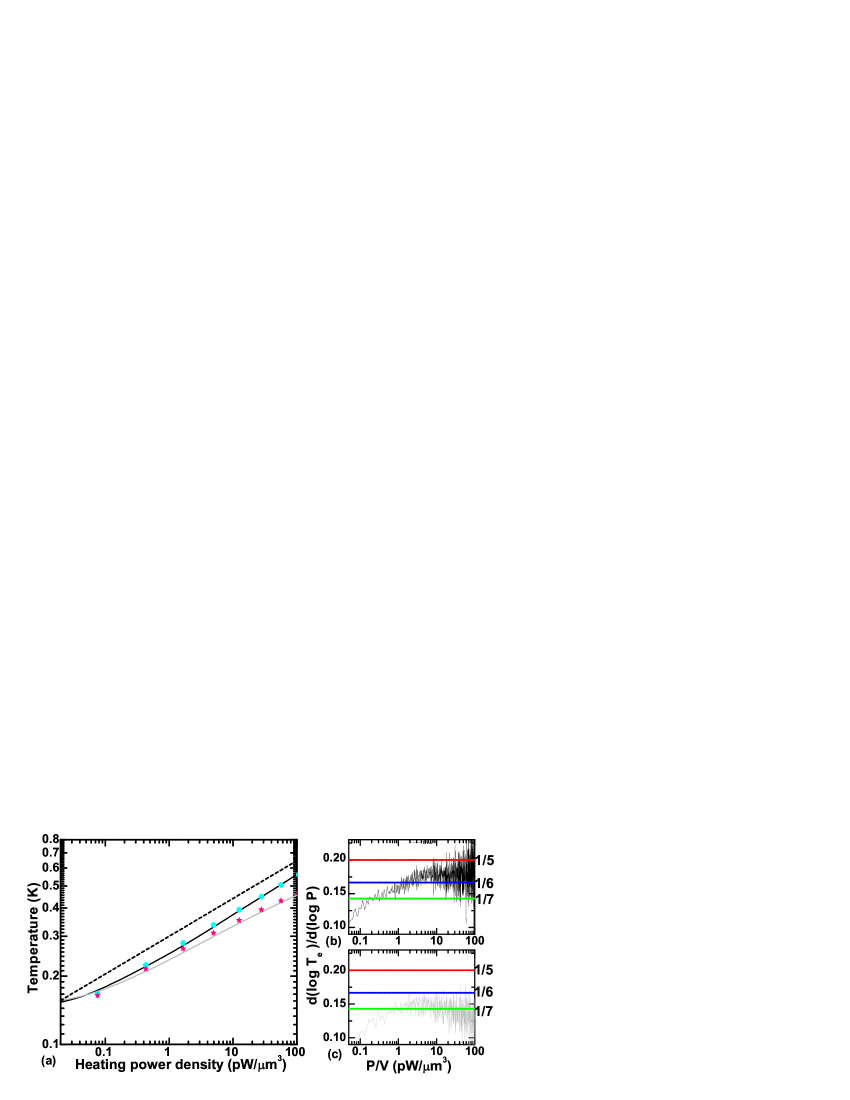
Figure 9: Data from the AlMn sample. Symbols are explained in the caption of Fig. 6.

The values for coupling constants $\Sigma$ can be determined from the slopes of the ($P/V,T$)-plots in logarithmic scale as fitting parameters, keeping $n$ fixed at $n=5$ or $n=6$. In Table 2 the measured values for $\Sigma$ are presented for all the samples. For Cu samples 1-3, $\Sigma$ decreases as a function of electron mean free path $l$; in other words, the electron-phonon interaction weakens with increased purity of the samples. This is evidence that the theory for pure electron-phonon coupling does not apply in our Cu thin films, although the temperature dependence agrees with the simplest theory without disorder.[11] Possible explanations for the experimental result $P\propto T^{5}$ are that our Cu samples are either in the transition region $ql\sim$ 1 or that the scattering potential is not fully vibrating. Our earlier conclusions[17, 19] on the temperature dependence of the electron-phonon coupling in disordered Cu and Au films were not correct, because the temperatures were measured with a side thermometer. For aluminum manganese samples with varying impurity concentration, $\Sigma$ is linearly dependent on $l$, consistent with the fully vibrating disorder theory.[18]

Table 2: Measured values for coupling constant $\Sigma$

	Cu sample 1	Cu sample 2	Cu sample 3	AlMn sample
$n$	5	5	5	6
$\Sigma$ [W/Knm3]	1.8 $\times 10^{9}$	2.1 $\times 10^{9}$	2.5 $\times 10^{9}$	3.4 $\times 10^{9}$

—

5 CONCLUSIONS

We have shown that thermal gradients are easily generated in mesoscopic samples at sub-Kelvin temperatures, even for good conductors such as copper. This fact has a strong effect on studies of thermal properties and thermometry. To obtain correct information on the electron-phonon interaction strength, for example, one has to make sure that electron temperature is measured in a location without thermal gradients. In addition, our results also imply that for tunnel junction coolers, large cold fingers outside the junction area are not effectively cooled. Also, even if the non-heated or non-cooled area is smaller than the electron-phonon scattering length $L_{e-p}$, thermal gradients will develop as long as the total size of the normal metal is of the order of $L_{e-p}$.

—

References

- [1] V. F. Gantmakher, Rep. Prog. Phys. 37, 317 (1974).
- [2] M. L. Roukes, M. R. Freeman, R. S. Germain, R. C. Richardson, and M. B. Ketchen, Phys. Rev. Lett. 55, 422 (1985).
- [3] J. M. Rowell, and D. C. Tsui, Phys. Rev. B 14, 2456 (1976).
- [4] F. Giazotto, T. T. Heikkilä, A. Luukanen, A. M. Savin and J. P. Pekola, Rev. Mod. Phys 78, 217 (2006).
- [5] D. R. Schmidt, R. J. Schoelkopf, and A. N. Cleland, Phys. Rev. Lett. 93, 045901 (2004).
- [6] M. Meschke, W. Guichard and J. P. Pekola, Nature 444, 187 (2006).
- [7] A. Schmid, Z. Phys. 259, 421 (1973).
- [8] M. Yu. Reizer and A. V. Sergeev, Zh. Eksp. Teor. Fiz. 90, 1056 (1986), [ Sov. Phys. JETP 63 616 (1986)].
- [9] A. Sergeev and V. Mitin, Phys. Rev. B 61, 6041 (2000).
- [10] M. Yu. Reizer, Phys. Rev. B 40, 5411 (1989).
- [11] F. C. Wellstood, C. Urbina, and J. Clarke, Phys. Rev. B 49, 5942 (1994).
- [12] R. Berman, Thermal Conduction in Solids, Clarendon Press, Oxford (1976).
- [13] A.H. Steinbach, J.M. Martinis, and M.H. Devoret, Phys. Rev. Lett. 76, 3806 (1996).
- [14] A.M. Clark, N.A. Miller, A. Williams, S.T. Ruggiero, G.C. Hilton, L.R. Vale, J.A. Beall, K.D. Irwin, and J.N. Ullom, Appl. Phys. Lett. 86, 173508 (2005).
- [15] A. Luukanen, M.M. Leivo, J.K. Suoknuuti, A.J. Manninen and J.P. Pekola, J. Low Temp. Phys. 120, 281 (2000).
- [16] N.A. Miller, A.M. Clark, A. Williams, S.T. Ruggiero, G.C. Hilton, J.A. Beall, K.D. Irwin, L.R. Vale, and J.N. Ullom, IEEE Trans. Appl. Supercond. 15, 556 (2005).
- [17] J.T. Karvonen, L.J. Taskinen and I.J. Maasilta, Phys. Rev. B 72, 012302 (2005).
- [18] L.J. Taskinen and I.J. Maasilta, Appl. Phys. Lett. 89, 143511 (2006).
- [19] J.T. Karvonen, L.J. Taskinen and I.J. Maasilta, Phys. Stat. Solidi C, 1, 2799 (2004).