Bond-Dilution-Induced Quantum Phase Transitions in Heisenberg Antiferromagnets

Abstract

Bond-dilution effects on the ground state of the square-lattice antiferromagnetic Heisenberg model, consisting of coupled bond-alternating chains, are investigated by means of the quantum Monte Carlo simulation. It is found that, when the ground state of the non-diluted system is a non-magnetic state with a finite spin gap, a sufficiently weak bond dilution induces a disordered state with a mid gap in the original spin gap, and under a further stronger bond dilution an antiferromagnetic long-range order emerges. While the site-dilution-induced long-range order is induced by an infinitesimal concentration of dilution, there exists a finite critical concentration in the case of bond dilution. We argue that this essential difference is due to the occurrence of two types of effective interactions between induced magnetic moments in the case of bond dilution, and that the antiferromagnetic long-range-ordered phase does not appear until the magnitudes of the two interactions become comparable.

1 Introduction

Randomness effects on quantum antiferromagnetic (AF) Heisenberg models with a spin-gapped ground state have attracted much interest in relation to the impurity-induced AF long-range order (LRO) observed experimentally, e.g., in the first inorganic spin-Peierls compound CuGeO₃ [1, 2], the two-leg ladder compound SrCu₂O₃ [3], and the Haldane compound PbNi₂V₂O₈ [4]. In the spin-Peierls compound CuGeO₃, the lattice dimerized state associated with a formation of spin gap is realized at low temperatures [1]. When a small amount of non-magnetic impurities Zn or Mg are substituted for Cu, the spin-gapped ground state of the pure system changes to an AF LRO state [5, 6, 7], thereby the lattice dimerization is preserved. Such an impurity-induced AF LRO has been observed also in the bond-disorder system, CuGe_1-xSi_xO₃ [2, 8, 9]. In early theoretical and numerical studies on quasi-one-dimensional diluted Heisenberg antiferromagnets, the effect of inter-chain interaction is often taken into account by making use of mean-field approximations, where the site and bond dilutions are unable to be distinguished with each other. [10, 11, 12] By the recent numerical analyses, however, the characteristic feature of the site-dilution-induced AF LRO has been understood more clearly by treating the inter- and intra-chain interactions on an equal footing. [13, 14, 15] More recently we have carried out extensive numerical simulations also on the bond-diluted system, and have found that the mechanism for the AF LRO to appear in this system is essentially different from that in the site-diluted system. The purpose of the present paper is to discuss our results in more detail, which have been reported in refs. yasuda2 and yasuda3 briefly.

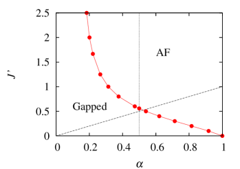
Figure 1: Ground state phase diagram of the non-diluted 2D $S=1/2$ AF Heisenberg model. The circles denote the phase boundary between the spin-gapped and AF LRO phases. The data points except for $\alpha=0.5$ were estimated by the previous quantum Monte Carlo simulation [20]. The error bar of each point is much smaller than the symbol size. The dotted and dashed lines denote $\alpha=0.5$ and $J^{\prime}=\alpha$, respectively.

In the present work we concentrate on the two-dimensional (2D) $S=1/2$ AF Heisenberg model consisting of coupled bond-alternating chains. The magnitude of the stronger (weaker) intra-chain interaction is put unity ($\alpha$) and that of the inter-chain interaction $J^{\prime}$ (see also Fig. 2 below). The ground state of decoupled chains, i.e., $J^{\prime}=0$, is the dimer state with a finite spin gap, $\Delta_{\rm p}$, except at the uniform point ($\alpha=1$) [18], which has a critical ground state with the Gaussian universality [19]. As $J^{\prime}$ increases, the quantum fluctuations, which invoked the dimer state, are gradually suppressed and the spin gap decreases. When $J^{\prime}$ exceeds a certain critical value, $J^{\prime}_{\rm c,p}$, which is a function of $\alpha$, the spin gap vanishes and the AF LRO emerges. A global ground state phase diagram, obtained by the previous quantum Monte Carlo simulation, [20] is presented in Fig. 1.

The ground state in the spin-gapped phase is described qualitatively well by a direct product state of singlet dimers sitting on each strong bond, which is called the valence-bond solid state. When spins are randomly removed (site dilution), a spin which formed a singlet pair formerly with a removed spin becomes nearly free. We call it an effectively free spin, or simply an effective spin. Due to the presence of weak interactions with the surrounding spins, an effective spin is somewhat blurred ; its linear extent is proportional to the correlation length of the non-diluted system. Between two effective spins at sites $m$ and $n$, there exists an effective interaction, ${\tilde{J}}_{mn}$, mediated by the sea of singlet pairs as illustrated in Fig. 2. It is either ferromagnetic or AF depending if $m$ and $n$ are on the same sublattice or on the different sublattices. It preserves its staggered nature with regard to the original square lattice and thus the dilution does not introduce frustration. In this sense we call $\{{\tilde{J}}_{mn}\}$ the effective AF interactions between effective spins. Its magnitude is finite, though exponentially small, even if $x$, the concentration of site dilution, is vanishingly small. Consequently, we expect $x_{\rm c}^{\rm s}$, the critical concentration of site dilution above which the disorder-induced AF LRO appears, is strictly zero. [13, 14, 15]

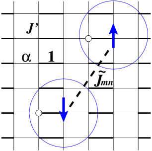
Figure 2: Effective spins (arrows) and an effective AF interaction in-between (${\tilde{J}}_{mn}$) in a site-diluted system. The thick and thin lines denote the strong and weak interactions, respectively, and the small circles represent the removed sites. The circles surrounding the arrows describe the extent of the effective spin schematically, which radius corresponds to the correlation length of the pure (i.e., non-diluted) system.

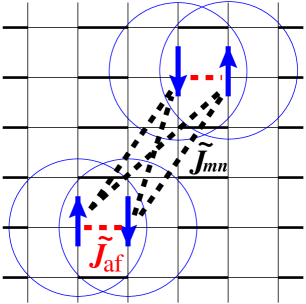
Figure 3: Two types of effective interactions ${\tilde{J}}_{mn}$ and ${\tilde{J}}_{\rm af}$ in the bond-diluted system. The former are mediated by the sea of singlet pairs as the same as the site-dilution case, whereas the latter act through the shortest 2D paths.

When a strong bond of amplitude unity is removed, on the other hand, two spins on the both edges of the removed bond become nearly free as shown in Fig. 3. We can also notice from the figure that there exists an effective AF interaction, ${\tilde{J}}_{\rm af}$, between these two spins, which is mediated mainly through the shortest paths of the interactions connecting them, i.e., ${\tilde{J}}_{\rm af}\sim J^{\prime 2}$. This interaction alone recombines the two spins to form a singlet pair with an excitation gap $\Delta$, which is proportional to ${\tilde{J}}_{\rm af}$. It yields a localized low-lying excited state, so-called mid-gap state, as long as $\Delta\ll\Delta_{\rm p}$. In the case of random bond dilution, in addition to ${\tilde{J}}_{\rm af}$, there also exist effective AF interactions, $\{{\tilde{J}}_{mn}\}$, between effective spins on edges of different removed bonds as in the site-diluted system (Fig. 3). Naturally, we expect competition between the two effective interactions, ${\tilde{J}}_{\rm af}$ and $\{{\tilde{J}}_{mn}\}$.

In the present paper, we discuss how the competition between these two types of interactions gives rise to the bond-dilution-induced AF LRO associated with a finite critical concentration of bond dilution, $x_{\rm c}\ (>0)$, in contrast to $x_{\rm c}^{\rm s}=0$ for the site dilution. We also investigate in some detail the mid-gap state due to ${\tilde{J}}_{\rm af}$ in the weak dilution limit, $x\rightarrow 0$, and shortly refer to a peculiar phenomenon which originates from the randomness in the system, namely, a possible existence of the quantum Griffiths phase neighboring to the AF LRO state.

The present paper is organized as follows. In §2, the model and the method of our numerical analyses are introduced. Detailed analyses of the mid-gap state in the limit of $x\to 0$ are presented in §3, and in §4 the ground state phase diagram on the $x$–$J^{\prime 2}$ plane is determined. Section 5 is devoted to summary and discussion.

2 Model and Numerical Method

We consider the bond-diluted quantum AF Heisenberg model on the square lattice of coupled bond-alternating chains. Its Hamiltonian is written as

$${\cal H} = \sum_{i,j}\epsilon_{(2i,j)(2i+1,j)}{\bf S}_{2i,j}\cdot{\bf S}_{2i+1,j}$$ (1)

$$+ \alpha\sum_{i,j}\epsilon_{(2i+1,j)(2i+2,j)}{\bf S}_{2i+1,j}\cdot{\bf S}_{2i+2,j}$$

$$+ J^{\prime}\sum_{i,j}\epsilon_{(i,j)(i,j+1)}{\bf S}_{i,j}\cdot{\bf S}_{i,j+1}\ ,$$

where 1 and $\alpha$ ($>0$) are the AF intra-chain alternating coupling constants, $J^{\prime}$ ($>0$) the AF inter-chain coupling constant, and ${\bf S}_{i,j}$ is the quantum spin operator with magnitude $S=1/2$ at site ($i,j$). We choose the $x$-axis as the one along chains and the $y$-axis as in the inter-chain direction. Randomly quenched bond occupation factors {$\epsilon_{(i,j)(k,l)}$} independently take either 1 or 0 with probability $1-x$ and $x$, respectively, where $x$ is the concentration of bond dilution.

The quantum Monte Carlo (QMC) simulations with the continuous-imaginary-time loop algorithm [21, 22] are carried out on $L\times L$ square lattices with periodic boundary conditions. For each sample with a bond-diluted configuration, $10^{3}\sim 10^{4}$ Monte Carlo steps (MCS) are spent for measurement after $5\times 10^{2}\sim 10^{3}$ MCS for thermalization. For each $x$ the random average is taken over $10^{1}\sim 10^{3}$ samples. As the temperature is decreased, each measured quantity, e.g., the structure factor, converges to a finite value. This reflects a finite excitation gap due to either of an intrinsic spin gap or the finiteness of the system. The simulations are performed at low enough temperatures, typically $T\simeq 10^{-3}$, where all the physical quantities of our interest do not show any temperature dependence and thus can be identified with those at the ground state.

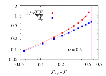
Figure 4: $J^{\prime}$ dependences of the the correlation lengths and the spin gap $\Delta_{\rm p}$ in the non-diluted system with $\alpha=0.5$, where $J^{\prime}_{\rm c,p}=0.5577(1)$ is the critical value of $J^{\prime}$ determined by the same method as in ref. matsumoto. The dotted line denotes $J^{\prime}=0$, the system of decoupled chains. The error bar of each point is smaller than the symbol size. The solid and dashed lines going through the data points are guides to eyes.

Before going into discussions on bond-diluted systems, let us here mention some ground state properties of the non-diluted systems described by Hamiltonian (1) with $x=0$. Its ground state phase diagram on the $\alpha$–$J^{\prime}$ plane is shown in Fig. 1. For discussions below we show in Fig. 4 the $J^{\prime}$ dependence of the spin gap $\Delta_{\rm p}$ and the inverse geometric mean of the correlation lengths $\xi_{\rm p}^{x}$ and $\xi_{\rm p}^{y}$ along $\alpha=0.5$, on which we concentrate our analyses of bond-dilution effects below. The correlation lengths $\xi_{\rm p}^{x}$ and $\xi_{\rm p}^{y}$ are estimated from the dynamical correlation functions at momenta $(\pi,0)$ and $(0,\pi)$, respectively, by using the second-moment method [23]. Similarly, $\Delta_{\rm p}$ is evaluated from the correlation function along the imaginary-time axis (see also below). As seen in Fig. 4, both $\Delta_{\rm p}^{-1}$ and $\xi_{\rm p}^{x}\xi_{\rm p}^{y}$ exhibit power law divergence as $J^{\prime}$ approaches $J^{\prime}_{\rm c,p}$ from below.

3 Mid-Gap State in the Limit of $x\to 0$

When a strong bond is removed from the non-diluted system with the non-magnetic ground state, two magnetic moments induced at the both ends of the diluted bond are expected to reform a spin singlet through ${\tilde{J}}_{\rm af}$, one of the effective AF interactions mentioned in §1. For a sufficiently weak bond dilution, $x\ll 1$, we expect a mid-gap state to appear, since the spin gap $\Delta$ induced by ${\tilde{J}}_{\rm af}$ is smaller than $\Delta_{\rm p}$, the spin gap in the non-diluted system. In this section, based on the QMC data, we discuss the $J^{\prime}$ dependence of the gap attributed to ${\tilde{J}}_{\rm af}$ in the limit of $x\to 0$.

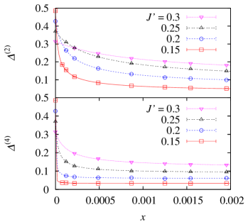
Figure 5: Dependences of $\Delta^{(2)}$ and $\Delta^{(4)}$ estimated by the second- and fourth-moment estimators on $x=1/(2L^{2})$ for $\alpha=0.5$ and $L\times L$ systems with $L=16$, 18, 20, 24, 32, 48, 64, and 80. The lines are the fitting functions [eqs. (5) and (7)].

To extract the value of $\Delta$, we make use of the second-moment formula, [22, 23]

$$(\Delta^{(2)})^{-1}=\frac{\beta}{2\pi}\sqrt{\frac{\tilde{C}(0)}{\tilde{C}(2\pi/\beta)}-1}\ .$$ (2)

Here $\beta$ is the inverse of temperature and $\tilde{C}(\omega)=\int_{0}^{\beta}{\rm d}\tau C(\tau)e^{i\omega\tau}$ is the Fourier transform of the imaginary-time staggered correlation function

$$C(\tau)\equiv\frac{1}{L^{2}}\sum_{i,j}(-1)^{|r_{i}-r_{j}|}\langle S_{i}^{z}(0)S_{j}^{z}(\tau)\rangle\ .$$ (3)

In the bond-diluted system of present interest, it is expected that $C(\tau)$ is dominated by two terms; the one representing the original spin gap in the non-diluted system and the one attributed to the mid gap. That is, the imaginary-time staggered correlation function can be approximated as [17, 24]

$$C(\tau) = a_{\rm p}\Big{[}{\rm cosh}\frac{\beta\Delta_{\rm p}}{2}\Big{]}^{-1}{\rm cosh}\{(\tau-\beta/2)\Delta_{\rm p}\}$$ (4)

$$+ a_{\rm i}\Big{[}{\rm cosh}\frac{\beta\Delta}{2}\Big{]}^{-1}{\rm cosh}\{(\tau-\beta/2)\Delta\}\ ,$$

where $a_{\rm p}$ and $a_{\rm i}$ are some functions of $\alpha$, $J^{\prime}$, and $x$. The coefficient $a_{\rm i}$, which represents the weight of the contribution from the mid-gap state, is naturally considered to be proportional to the concentration of diluted bonds, i.e., $a_{\rm i}=ax$ with $a=a(\alpha,J^{\prime})$. From eqs. (2), (4), and $a_{\rm p}+a_{\rm i}=1$, $\Delta^{(2)}$ is evaluated as

$$\Delta^{(2)}=\Delta\sqrt{(1+\frac{1-ax}{ax}\frac{\Delta}{\Delta_{\rm p}})/\{{1+\frac{1-ax}{ax}(\frac{\Delta}{\Delta_{\rm p}})^{3}}\}}$$ (5)

for $\beta^{-1}\ll\Delta\ll\Delta_{\rm p}$. Note that in the last expression, $\Delta^{(2)}$ explicitly depends on $x$ as well as on $\Delta$. We regard eq. (5) as a fitting function to extract $\Delta$ in the weak dilution limit, where $\Delta$ is assumed to be independent of $x$.

The QMC simulation to evaluate $\Delta^{(2)}$ is performed along $\alpha=0.5$ for the system with only one diluted bond, which corresponds to the $x=1/2L^{2}$ system. By taking the limit of $L\to\infty$, we can investigate the properties in the limit of $x\to 0$. The obtained set of $\Delta^{(2)}(x)$ for each $J^{\prime}$ is fitted by eq. (5), thereby the value of $\Delta_{\rm p}$ is fixed to the one simulated in the non-diluted system. In the upper part of Fig. 5 the $x$ dependence of $\Delta^{(2)}$ is presented. The resultant spin gap $\Delta$ is shown in Fig. 6. As a function of $J^{\prime}$, it increases proportionally to $J^{\prime 2}$, while $\Delta_{\rm p}$ decreases (see Fig. 4).

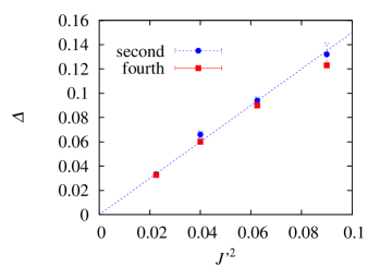
Figure 6: $J^{\prime 2}$ dependences of the spin gap estimated by the second- and fourth-moment estimators. The dashed line, which represents $\Delta=1.5J^{\prime 2}$, is a guide to eyes.

We have further confirmed the values of $\Delta$ by using the fourth-moment estimator [22], defined by

$$(\Delta^{(4)})^{-1}=\frac{\beta}{4\pi}\sqrt{3\frac{\tilde{C}(0)-\tilde{C}(2\pi/\beta)}{\tilde{C}(2\pi/\beta)-\tilde{C}(4\pi/\beta)}-1}\ .$$ (6)

In this case the fitting function becomes

$$\Delta^{(4)}=\Delta\sqrt{\{{1+\frac{1-ax}{ax}(\frac{\Delta}{\Delta_{\rm p}})^{3}\}/\{1+\frac{1-ax}{ax}(\frac{\Delta}{\Delta_{\rm p}})^{5}}\}}\ .$$ (7)

The lower part of Fig. 5 is the $x$ dependence of $\Delta^{(4)}$ obtained by eq. (6). It is observed that as $x$ increases $\Delta^{(4)}$ converges more rapidly to a constant values, which corresponds to $\Delta$. This is due to the smaller corrections, $[(1-ax)/ax](\Delta/\Delta_{\rm p})^{3}$, in eq. (7) than those for $\Delta^{(2)}$.

Figure 6 shows a nice coincidence of the values of $\Delta$, estimated by the second- and fourth-moment methods. We therefore conclude the existence of a mid-gap state whose gap $\Delta$ is proportional to $J^{\prime 2}$ and distinctly smaller than $\Delta_{\rm p}$, and whose contribution to the imaginary-time correlation function is proportional to $x$. This is just what we have expected, i.e., a reformed singlet pair due to the effective AF interaction ${\tilde{J}}_{\rm af}$ acting on two effective spins at both ends of a diluted strong bond.

4 Bond-Dilution-Induced Antiferromagnetic Long-Range-Ordered Phase

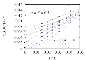
Figure 7: System size dependences of $S_{\rm s}(L,0,x)/L^{2}$ for $x=0.02$ (crosses), 0.04 (x-marks), 0.06 (squares), 0.08 (circles), 0.1 (upward triangles), 0.2 (downward triangles), 0.3 (diamonds), and 0.35 (pentagons) at $(\alpha,J^{\prime})=(0.5,0.5)$. Dashed lines are obtained by the least-squares fitting. The extrapolated values are denoted by the filled symbols which correspond to $M_{\rm s}^{2}/3$ in the thermodynamic limit.

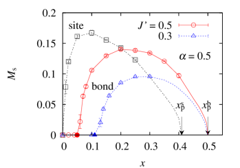
Figure 8: Dependences of the staggered magnetization on the concentration of bond dilution for $(\alpha,J^{\prime})=(0.5,0.5)$ and $(0.5,0.3)$. The solid circle and triangle denote the quantum critical points, $x_{\rm c}\approx 0.0502$ and 0.1101, respectively, estimated by the finite-size scaling analysis described in the text. For comparison, we also show the result of the site dilution for $(\alpha,J^{\prime})=(0.5,0.5)$, which is taken from ref. 15. The percolation thresholds on the site and bond processes are denoted by $x_{\rm p}^{\rm s}\approx 0.41$ and $x_{\rm p}^{\rm b}=0.5$, respectively. All the lines are guides to eyes.

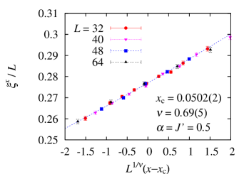
(a)       (b)

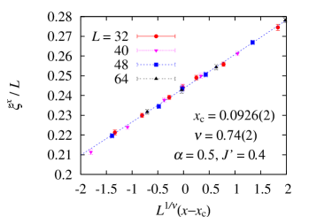
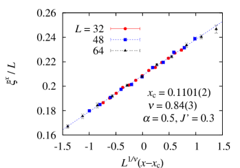
(c)       (d)

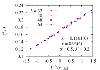
Figure 9: Finite-size scaling plots of the correlation length for (a) $(\alpha,J^{\prime})=(0.5,0.5)$, (b) $(0.5,0.4)$, (c) $(0.5,0.3)$, and (d) $(0.5,0.2)$.

As $x$ is increased from zero, fitting of $C(\tau)$ by using eq. (4) becomes unstable, implying that a number of mid-gap states, other than $\Delta$ discussed in the previous section, appear. We have clearly observed, however, that $\Delta^{(2)}$ of eq. (2), which we now regard as an upper bound of the spin gap, as well as the inverse of the spatial correlation lengths, $\xi^{x}$ and $\xi^{y}$, decrease as $x$ increases. [17] Finally, when $x$ exceeds a certain critical value, $x_{\rm c}$, the AF LRO appears. During the present section, we call the state between $x=0$ and $x_{\rm c}$ simply the disordered state, and concentrate on the quantum phase transition at $x=x_{\rm c}$ to the AF LRO state, postponing the discussion about a possible existence of the quantum Griffiths state at $x<x_{\rm c}$ until the last section.

To discuss the quantum phase transition between the disordered and the AF LRO phases, first we investigate the zero-temperature staggered magnetization, $M_{\rm s}$, as a function of $x$, which is evaluated as

$$M_{\rm s}^{2}(x)=\lim_{L\to\infty}\lim_{T\to 0}\frac{3S_{\rm s}(L,T,x)}{L^{2}}\ .$$ (8)

Here $S_{\rm s}(L,T,x)$, the static structure factor at momentum $(\pi,\pi)$, is defined by

$$S_{\rm s}(L,T,x)\equiv\frac{1}{L^{2}}\sum_{i,j}(-1)^{|r_{i}-r_{j}|}\langle S_{i}^{z}S_{j}^{z}\rangle\ .$$ (9)

In Fig. 7 we show the system size dependence of $S_{\rm s}(L,0,x)/L^{2}$ for various $x$’s. For $x\geq 0.06$, the QMC data for each $x$ are fitted fairly well by a linear expression, $a+bL^{-1}$, where the value of $a$, represented by the solid symbols in the figure, gives an estimate for $M_{\rm s}^{2}/3$ in the thermodynamic limit. For $x=0.02$ and 0.04, on the other hand, we find a linear fit extrapolates to a negative $M_{\rm s}^{2}/3$ for $L\to\infty$, which indicates a vanishing staggered magnetization. Indeed, the data are fitted much better by $S_{\rm s}(L,0,x)=a(1-{\rm exp}(-bL))$, which is the scaling form derived for a non-magnetic ground state in the modified spin-wave theory. [25]

In Fig. 8 the $x$ dependences of $M_{\rm s}$ are shown for $J^{\prime}=0.3$ and 0.5, together with that for the site-diluted system [15] for comparison. The value of $\alpha$ is fixed to be 0.5 in all the cases. It is clearly demonstrated that while the AF LRO is induced at an infinitesimal concentration of site dilution, in the bond-diluted system there exists a critical concentration, e.g., $x_{\rm c}\approx 0.11$ for $J^{\prime}=0.3$. It is also definitely finite even for $J^{\prime}=0.5$, whose non-diluted system is close to the critical point $J^{\prime}_{\rm c,p}\approx 0.5577$.

In passing we note that $M_{\rm s}(x)$ shown in Fig. 8 has a peak at $x=x_{\rm opt}$. In the strong dilution regime, $x_{\rm opt}\lesssim x\leq x_{\rm p}^{\rm s,b}$, the further dilution tends to destroy the AF LRO and the latter would vanish just at the percolation threshold [26, 27].

Next let us determine the phase diagram on the $x$–$J^{\prime 2}$ plane. The critical concentration of dilution, $x_{\rm c}$, which is roughly evaluated above, is estimated more precisely by the finite-size scaling analysis of the correlation length $\xi^{x}$ as shown in Fig. 9. The critical concentrations are estimated as $x_{\rm c}=0.0502(2)$, 0.0926(2), 0.1101(2), and 0.1161(6) for $J^{\prime}=0.5$, 0.4, 0.3, and 0.2, respectively. [Almost the equal values of $x_{\rm c}$ are obtained by the same analysis on $\xi^{y}$.] The values of the critical exponent of the correlation length are $\nu=0.69(5)$, 0.74(2), 0.84(3), and 0.95(4), respectively, which monotonically increases from $\nu=0.71$, the critical exponent of the three-dimensional classical Heisenberg universality class. [28] We note, however, that the finite-size scaling analysis with the fixed critical exponent $\nu=0.71$ gives the same value of $x_{\rm c}$ within the numerical accuracy. Certainly, more precise numerical data are needed to settle this point.

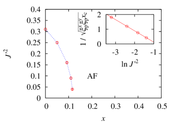
Figure 10: Phase diagram of the ground state for $\alpha=0.5$. The circles are evaluated by the finite-size scaling analysis. The dashed line is a guide to eyes. In the inset we show the relation between $1/\sqrt{\xi_{\rm p}^{x}\xi_{\rm p}^{y}x_{\rm c}}$ and $\ln{J^{\prime 2}}$, where we used the QMC data ($\xi_{\rm p}^{x},\xi_{\rm p}^{y}$) = (11.998(9), 9.312(10)), (5.320(1), 3.460(2)), (3.452(1), 1.8202(3)), and (2.5492(4), 1.03244(5)) for $J^{\prime}=0.5$, 0.4, 0.3, and 0.2, respectively. The straight line in the inset represents a linear fitting of the data by $y=a+bx$ with $a=-0.633(6)$ and $b=-0.762(3)$.

The resultant phase diagram is shown in Fig. 10. In the inset of the figure we show an important result, i.e., the relation of $x_{\rm c}$ to $J^{\prime 2}$, or the inverse of the function $J^{\prime}_{\rm c}(x)$, a critical value of $J^{\prime}$ for a given $x$ (and a given $\alpha$). Note that $J^{\prime}_{\rm c,p}=J^{\prime}_{\rm c}(x=0)$. The effective AF interaction, $\tilde{J}_{mn}$, introduced in §1 is approximately described by

$$\tilde{J}_{mn}\propto(-1)^{|r_{m}-r_{n}+1|}{\rm exp}(-\frac{\ell}{\sqrt{\xi_{\rm p}^{x}\xi_{\rm p}^{y}}})\ ,$$ (10)

where $\ell=|r_{m}-r_{n}|$ is the distance between the effective spins [29, 30] at the ends of different removed bonds. On the other hand, the effective AF interaction, $\tilde{J}_{\rm af}$, between effective spins on the same removed bond is simply described by

$$\tilde{J}_{\rm af}\simeq J^{\prime 2}\ .$$ (11)

Thus the relation indicated in the inset of Fig. 10 is read as

$${\cal J}(x_{\rm c})\simeq\tilde{J}_{\rm af}\ ,$$ (12)

where ${\cal J}(x)$ is an average of $\{{\tilde{J}}_{mn}\}$ acting on effective spins on neighboring diluted bonds, and is approximately represented as

$${\cal J}(x)\simeq{\cal J}_{0}\ {\rm exp}(-\frac{1}{\sqrt{\xi_{\rm p}^{x}\xi_{\rm p}^{y}x}})\ ,$$ (13)

in which the exponential part is obtained from $\tilde{J}_{mn}$ of eq. (10) with $1/\sqrt{x}$, i.e., the mean distance of the nearest removed bonds, substituted for $\ell$. The result of eq. (12) implies that the phase transition between the disordered and AF LRO phases occurs when the magnitudes of $\tilde{J}_{\rm af}$ and ${\cal J}(x)$ become comparable. We interpret this result as described below.

Let us replace a bond-diluted system of present interest by a model system consisting only of effective spins with interactions $\{{\tilde{J}}_{mn}\}$ and ${\tilde{J}}_{\rm af}$, neglecting all spins in the sea of singlet pairs. Since $\{{\tilde{J}}_{mn}\}$ do not introduce frustration at all, combined with the fact that $\{{\tilde{J}}_{mn}\}$ are short-ranged except for the system with $J^{\prime}=J^{\prime}_{\rm c,p}$, the actual geometry of $\{{\tilde{J}}_{mn}\}$ is not relevant to the present problem, and so we may further simplify the model system to a regular square array of the effective spins; along the chain direction the interactions are alternating between ${\tilde{J}}_{\rm af}$ and ${\cal J}(x)$, while in the inter-chain direction the interaction is uniform, i.e., also ${\cal J}(x)$ given above. In this way, the original system in the disordered state can be approximately mapped to a gapped state of the original non-diluted system of Fig. 1 but with both $\alpha$ and $J^{\prime}$ replaced by ${\cal J}(x)/\tilde{J}_{\rm af}$. As $x$ (and/or $J^{\prime}$) of the bond-diluted system increases, ${\cal J}(x)/{\tilde{J}}_{\rm af}$ does so, which corresponds to the upward movement of the mapped regular system along the dashed line ($J^{\prime}=\alpha$) in the figure. Finally it hits the critical line at $x=x_{\rm c}(J^{\prime})$ ($J^{\prime}=J^{\prime}_{\rm c}(x)$), where eq. (12) holds, and the quantum phase transition to the AF LRO phase occurs.

Our above scenario can explain the behavior of the critical line in the $x\rightarrow 0$ limit, i.e., $J^{\prime}_{\rm c}(x)$ at least first decreases from $J^{\prime}_{\rm c,p}$ when the dilution is introduced (see Fig. 10). Naively one might expect the dilution suppresses the bulk correlation represented by $\xi_{\rm p}^{x,y}$, and in order to recover this decrease, the stronger $J^{\prime}$ is needed for the AF LRO to appear, yielding an initial increase of $J^{\prime}_{\rm c}(x)$. If, however, our scenario is applied to the system just at $J^{\prime}=J^{\prime}_{\rm c,p}$, where the correlation lengths $\xi_{\rm p}^{x,y}$ are infinite, it is expected that the AF LRO is induced by an infinitesimal concentration of dilution, since $\{J_{mn}\}$ is quasi-long-ranged even for a vanishingly small $x$ and the prefactor in eq. (13), ${\cal J}_{0}$, depends more weakly on $J^{\prime}$ than ${\tilde{J}}_{\rm af}\ (\propto J^{\prime 2})$ does. This means that $J^{\prime}_{\rm c}(x)$ has a negative slope at least at $x=0^{+}$. Actually, from eqs. (12) and (13) combined with the critical behavior of $\xi_{\rm p}^{x,y}$ at $J^{\prime}\simeq J^{\prime}_{\rm c,p}$, the decrease of $J^{\prime}_{\rm c}(x)$ at $x\sim 0$ is deduced. However, quantitative details of its behavior in the weak dilution limit are beyond a scope of the present work.

5 Conclusion and Discussion

In the present paper, we have investigated the bond-dilution effects on the non-magnetic ground state of the 2D quantum AF Heisenberg model consisting of bond-alternating chains by means of the QMC simulations, and have proposed a scenario that the quantum phase transition induced by bond dilution is originated from the competition of the two effective AF interactions $\{{\tilde{J}}_{mn}\}$ and ${\tilde{J}}_{\rm af}$. In particular, the proposed simple mapping of a bond-diluted system to a non-diluted system catches up the essential mechanism of the bond-dilution-induced AF LRO in the system so long as the effective interaction ${\cal J}(x)$, which represents an averaged value of $\{{\tilde{J}}_{mn}\}$, is less than or comparable to ${\tilde{J}}_{\rm af}$, or in other words, $J^{\prime}$ is not too small.

In our arguments so far described, we have kept away from an interesting problem whether the disordered state in the present system may involve a novel aspect of quantum random systems such as the quantum Griffiths (QG) phase or not. By our scenario with the averaged interaction ${\cal J}(x)$ we completely neglect this possibility. For $J^{\prime}=0$, i.e., the system is exactly one-dimensional, the system with $0<x<1$ is known to be in the QG phase characterized by finite correlation lengths but with a continuous distribution of spin gaps up to zero. [31, 32, 33, 34]. If this QG state is unstable against the AF LRO state due to the introduction of $J^{\prime}$ even of an infinitesimal magnitude, the latter state invades to $x\rightarrow 0$, i.e., a reentrant transition from the disordered state to the AF LRO state as decreasing $J^{\prime}$ is expected for $x$ smaller than 0.11. Also for a moderate value of $J^{\prime}$ for which we have observed the quantum phase transition from the disordered state to the AF LRO state, there remains the problem of a possible existence of the QG state. Actually in our preliminary analysis we observed in the $J^{\prime}=0.3$ system that $\Delta^{(2)}$ of eq. (2) decreases much faster than the inverse of the spatial correlation length as $x$ increases. [17] This strongly suggests an existence of the QG state. However, in order to confirm a continuous distribution of spin gaps up to zero, we have to carry out QMC simulations at correspondingly low temperatures. This problem as well as that of the possible reentrant transition mentioned above remain as challenging future works in the field of the computational physics.

In order to distinguish experimentally the characteristic difference between the site- and bond-dilution-induced AF LRO states pointed out in the present work, one needs a suitable material; a quasi-one-dimensional Heisenberg antiferromagnet with small enough $J^{\prime}$ and rigid bond alternation, and without frustration. Furthermore these properties are desired not to change significantly by dilution processes. In the spin-Peierls compound CuGe_1-xSi_xO₃, which is effectively a bond-disorder Heisenberg antiferromagnet [2], it was experimentally observed that the effective spins are induced not near Si impurity sites but rather at sites between them in the AF LRO phase [9]. The occurrence of the AF LRO is then attributed to the nonlocal reconstruction of bond alternation by Si substitution. To understand this type of phase transitions in the spin-Peierls state, we have to analyze models with proper spin-lattice coupling, which will be another challenging numerical work in near future.

References

- [1] M. Hase, I. Terasaki and K. Uchinokura: Phys. Rev. Lett. 70 (1993) 3651.
- [2] L. P. Regnault, J. P. Renard, G. Dhalenne and A. Revcolevschi: Europhys. Lett. 32 (1995) 579.
- [3] M. Azuma, Y. Fujishiro, M. Takano, M. Nohara and H. Takagi: Phys. Rev. B 55 (1997) R8658.
- [4] Y. Uchiyama, Y. Sasago, I. Tsukada, K. Uchinokura, A. Zheludev, T. Hayashi, N. Miura and P. Böni: Phys. Rev. Lett. 83 (1999) 632.
- [5] M. C. Martin, M. Hase, K. Hirota, G. Shirane, Y. Sasago, N. Koide and K. Uchinokura: Phys. Rev. B 56 (1997) 3173.
- [6] T. Masuda, A. Fujioka, Y. Uchiyama, I. Tsukada and K. Uchinokura: Phys. Rev. Lett. 80 (1998) 4566.
- [7] K. Manabe, H. Ishimoto, N. Koide, Y. Sasago and K. Uchinokura: Phys. Rev. B 58 (1998) R575.
- [8] T. Masuda, K. Ina, K. Hadama, I. Tsukada, K. Uchinokura, H. Nakao, M. Nishi, Y. Fujii, K. Hirota, G. Shirane, Y. J. Wang, V. Kiryukhin and R. J. Birgeneau: Physica B 284-288 (2000) 1637.
- [9] J. Kikuchi, T. Matsuoka, K. Motoya, T. Yamauchi and Y. Ueda: Phys. Rev. Lett. 88 (2002) 037603.
- [10] S. Miyashita and S. Yamamoto: Phys. Rev. B 48 (1993) 913.
- [11] S. Eggert and I. Affleck: Phys. Rev. Lett. 75 (1995) 934.
- [12] H. Fukuyama, T. Tanimoto and M. Saito: J. Phys. Soc. Jpn. 65 (1996) 1182.
- [13] M. Imada and Y. Iino: J. Phys. Soc. Jpn. 66 (1997) 568.
- [14] S. Wessel, B. Normand, M. Sigrist and S. Haas: Phys. Rev. Lett. 86 (2001) 1086.
- [15] C. Yasuda, S. Todo, M. Matsumoto and H. Takayama: Phys. Rev. B. 64 (2001) 092405.
- [16] C. Yasuda, S. Todo, M. Matsumoto and H. Takayama: J. Phys. Chem. Solids 63 (2002) 1607.
- [17] C. Yasuda, S. Todo, M. Matsumoto and H. Takayama: Prog. Theor. Phys. Suppl. 145 (2002) 339.
- [18] L. N. Bulaevskii: Sov. Phys. JETP 17 (1963) 684; J. C. Bonner, H. W. J. Blöte, J. W. Bray and I. S. Jacobs: J. Appl. Phys. 50 (1979) 1810.
- [19] I. Affleck and F. D. M. Haldane: Phys. Rev. B 36 (1987) 5291.
- [20] M. Matsumoto, C. Yasuda, S. Todo and H. Takayama: Phys. Rev. B. 65 (2002) 014407.
- [21] H. G. Evertz, G. Lana and M. Marcu: Phys. Rev. Lett. 70 (1993) 875; B. B. Beard and U.-J. Wiese: Phys. Rev. Lett. 77 (1996) 5130.
- [22] S. Todo and K. Kato: Phys. Rev. Lett. 87 (2001) 047203.
- [23] F. Cooper, B. Freedman and D. Preston: Nucl. Phys. B 210 [FS6] (1982) 210.
- [24] The prefactors in eq. (3.4) in ref. \citenyasuda3 should be read respectively for and . The following equations and discussions in ref. \citenyasuda3 are not affected by these typographic errors.
- [25] M. Takahashi: Phys. Rev. B 40 (1989) 2494.
- [26] K. Kato, S. Todo, K. Harada, N. Kawashima, S. Miyashita and H. Takayama: Phys. Rev. Lett. 84 (2000) 4204.
- [27] S. Todo, C. Yasuda, K. Kato, K. Harada, N. Kawashima, S. Miyashita and H. Takayama: Prog. Theor. Phys. Suppl. 138 (2000) 507.
- [28] K. Chen, A. M. Ferrenberg and D. P. Landau: Phys. Rev. B 48 (1993) 3249.
- [29] N. Nagaosa, A. Furusaki, M. Sigrist and H. Fukuyama: J. Phys. Soc. Jpn. 65 (1996) 3724.
- [30] Y. Iino and M. Imada: J. Phys. Soc. Jpn. 65 (1996) 3728.
- [31] D. S. Fisher: Phys. Rev. B 50 (1994) 3799.
- [32] R. A. Hyman, K. Yang, R. N. Bhatt and S. M. Girvin: Phys. Rev. Lett. 76 (1996) 839.
- [33] K. Hida: J. Phys. Soc. Jpn. 65 (1996) 895; 65 (1996) 3412(E); 66 (1997) 3237.
- [34] S. Todo, K. Kato and H. Takayama: Computer Simulation Studies in Condensed-Matter Physics XI, ed. D. P. Landau and H.-B. Schüttler (Springer, Berlin, Heidelberg, 1999) p. 57.
- [35] http://wistaria.comp-phys.org/looper/