Observing Majorana Bound States in p-wave Superconductors Using Noise Measurements in Tunneling Experiments

Abstract

The zero-energy bound states at the edges or vortex cores of chiral p-wave superconductors should behave like Majorana fermions. We introduce a model Hamiltonian that describes the tunnelling process when electrons are injected into such states. Using a non-equilibrium Green function formalism, we find exact analytic expressions for the tunnelling current and noise and identify experimental signatures of the Majorana nature of the bound states to be found in the shot noise. We discuss the results in the context of different candidate materials that support triplet superconductivity. Experimental verification of the Majorana character of midgap states would have important implications for the prospects of topological quantum computation.

When the individual constituents of a many-body system interact non-trivially with each other, they can give rise to low-energy states in which the elementary excitations are very different from the original building blocks. Examples among electronic condensed-matter systems include the spinons and holons in Luttinger liquids (realized, e.g., in single-wall carbon nanotubes) or the Laughlin quasiparticles of fractional quantum Hall systems. In the context of superconductors, Cooper pairs can be seen as a relatively simple example of such excitations, but more exotic states are also possible. In the present work we are interested in the case of p-wave chiral superconductors (i.e. with an order parameter of the type $\hat{p}_{x}\pm i\hat{p}_{y}$), examples of which would be strontium ruthenate (Sr₂RuO₄) Murakawa et al. (2004); Xia et al. (2006) and, possibly, a number of organic superconductors like the Bechgaard salts ({TMTSF}₂X; X$=$PF₆,ClO₄,…) che (2004), and even heavy fermions (e.g. UPt₃) Tou et al. (1996).

Superconductors with p-wave orbital symmetry have spin-triplet pairing and the order parameter is a tensor in spin space rather than a scalar. This introduces extra freedom and allows for different types of superconducting phases, first studied and observed in superfluid ³He. In the so called A-phase, Cooper pairs are in a state dubbed ‘equal (or parallel) spin pairing’ (ESP); all the examples given above are candidate systems for ESP. Within weak-coupling BCS theory the up- and down-spin sectors are then independent from each other and the respective Bogoliubov-de Gennes (BdG) equations are decoupled. Another aspect of the A-phase of p-wave superconductors is that it can support vortex-core bound states with a spectrum given by $E_{n}=-\omega_{0}\left(n+\tilde{n}\right)$ with $n\in\mathbb{Z}$, $\tilde{n}=0$ and $\omega_{0}$ a frequency that depends on the details of the vortex profile Kopnin and Salomaa (1991). In particular, for $n=0$, one notices that the vortices support ‘zero modes’. (This should be contrasted with the case of s-wave superconductors for which the vortex bound-state spectrum has again the same form but this time $\tilde{n}=1/2$, the other of the only two possibilities consistent with the $E\rightarrow-E$ symmetry of the BdG equations.) A more detailed consideration of these midgap bound states in the case of ESP reveals that they have self-adjoint wavefunctions, naturally described as Majorana fermion modes, and can also be found as edge states Read and Green (2000). Such Majorana states constitute one more example of an exotic low-energy collective excitation that is very different from the original electrons that condensed into the superconducting state.

It would be already extremely interesting to be able to experimentally identify these strange Majorana bound states, since that would constitute a stringent test of our current picture of EPS p-wave superconductivity, but the motivations run further. The availability of Majorana fermions can be exploited in the context of quantum computation, a completely new and revolutionary approach to computing that would mix aspects of the digital and the analog computing paradigms by exploiting the basic laws of quantum mechanics. Majorana operators (call them $\eta_{i}$) can be taken in pairs to define standard fermionic operators [say, $c^{\dagger}=\left(\eta_{r}+i\eta_{l}\right)/\sqrt{2}$]; each of these generates a two-dimensional Hilbert space that can be used to define a quantum-bit (qubit). Because the two Majoranas can be spatially far apart (e.g. in two different vortices) and are very different from the usual fermionic quasiparticles around them, the so defined qubit would be relatively immune to decoherence Ivanov (2001), which would sidestep one of the crucial problems faced by the development of quantum computing hardware. Moreover, it turns out that the usual global gauge symmetry of the fermi fields is reduced to a discrete $\mathbf{Z}_{2}$ symmetry for the Majoranas at the core of a vortex (and they can be shown to change sign when a third vortex moves about encircling them Ivanov (2001); Stone and S.-B. Chung (2006)). Changing the sign of a single Majorana of the pair that defines a qubit operates the change $c^{\dagger}\rightleftarrows c$, or, in other words, it acts as a qubit-flip (or q-NOT) gate, and the $\mathbf{Z}_{2}$ symmetry being discrete leaves no room for errors. This shows that braiding vortices would perform quantum-logical operations on the information stored in them, an approach known as topological quantum computation (for a recent review see Ref. Das Sarma et al., 2006).

Recently, the overlap matrix element between a localized electron and a Majorana bound state was computed for a model of a superconducting wire (introduced in the context of quantum computation A. Yu. Kitaev (2000)) and found to be non-zero Semenoff and Sodano (2006). This indicates that tunnelling transport into Majorana modes is possible, which opens interesting possibilities since tunnelling has proved repeated times to be an invaluable tool in the study of superconducting states. The study of tunnelling noise might also be useful, since shot noise is another probe able to distinguish normal versus superconducting states and ballistic versus diffusive transport Fauchère et al. (1998); Blanter and Büttiker (2000); it can also be sensitive to the charge and statistics of the carriers and was used, for instance, to confirm the presence of Laughlin quasiparticles in fractional quantum Hall devices Saminadayar et al. (1997). Noise probes can be local, in order to study localized states Birk et al. (1995). The purpose of this article is to model the tunnelling processes into Majorana bound states and to determine the current and noise characteristics in order to identify signatures that would allow the experimental identification and study of such states. A generalized geometry of the experiment we consider is shown in Fig. 1. We shall find that the Fano factor (or shot noise to current ratio) for such tunnelling processes has unit matrix structure and is given by

$$F_{\alpha\beta}\equiv\lim_{V/T\rightarrow\infty}\frac{S_{\alpha\beta}\left(\omega=0\right)}{e\left(I_{\alpha}+I_{\beta}\right)}=\delta_{\alpha\beta}$$ (1)

where $\alpha,\beta=\left\{L,R\right\}=\pm 1$ label the lead where the currents ($I_{\alpha,\beta}$) are measured and $S_{\alpha\beta}$ is the noise spectrum defined below. This is different from the result for a regular fermionic bound state for which $F_{\alpha\beta}=1/2$ has a ‘flat’ matrix structure and is half as big –the full expressions for the noise are given in Eqs. (2) and (3)–. We shall argue that measuring the Fano factor would provide a clear signature of the Majorana nature of a bound state.

The current-voltage characteristics for tunnelling into low-dimensional chiral p-wave superconductors was computed before for the case of planar junctions using a BTK formalism (including the bound states in a density of states approximation) Sengupta et al. (2001), or for point contacts using a microscopic tunnelling Hamiltonian and non-equilibrium Green functions but in the absence of bound states (i.e. far from vortices or edges) Bolech and Giamarchi (2004). Here we concentrate on the tunneling into bound states or edge modes for voltages smaller than the superconducting gap and carry out full microscopic calculations for the current as well as the noise. Our starting point is the following tunnelling Hamiltonian:

$$H=H_{0}+\sqrt{2}t_{L}~{}i\eta_{l}\left(\psi_{L}^{\dagger}+\psi_{L}\right)+\sqrt{2}t_{R}\left(\psi_{R}^{\dagger}-\psi_{R}\right)\eta_{r}$$

here $\eta_{r,l}$ are two different Majorana operators (located, for instance, in two different vortices; see Fig. 1) and $\psi_{\alpha}^{\dagger}=\int\psi_{\alpha k}^{\dagger}dk/2\pi$ are the fermions at the position of the point contact in each of two leads. We consider only the relevant spin projection of the ESP state and effectively work with spinless fermions. The $H_{0}$ term in the Hamiltonian has two parts,

$$H_{0,\alpha}=\int\frac{dk}{2\pi}~{}\varepsilon_{k}~{}\psi_{\alpha k}^{\dagger}\psi_{\alpha k}\quad\text{and}\quad H_{0,c}=\varepsilon~{}i\eta_{l}\eta_{r}{\small\rightarrow}\varepsilon~{}c^{\dagger}c~{}\text{,}$$

where $c^{\dagger}$ is defined as above and there is a term $H_{0,\alpha}$ for each lead. $H_{0,c}$ serves to model the case when the overlap matrix element between the two Majorana bound states is non-zero (cf. Ref. Semenoff and Sodano, 2006). Notice that the terms in $H$ involving $\eta$’s are bound to have the form they have due to hermiticity requirements (cf. Ref. Stone and S.-B. Chung, 2006). The overlap amplitudes $t_{\alpha}$ have to be real and we can take them to be positive for the sake of concreteness. The choice of relative signs in the tunnelling terms is arbitrary and amounts to a choice of global gauges for the leads.

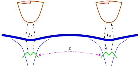
Figure 1: Schematic representation of our model for a setup in which two contacts (e.g. two STM tips) tunnel electrons into the Majorana bound states at the core of vortices. The two Majorana states might be linked with a tunnelling amplitude $\varepsilon$. The setup is generic and any or both of the vortices could be replaced by edge modes or obviated altogether. The model would also apply to the case of multiband vortices with two different Majoranas one on each band, in such a case $\varepsilon$ corresponds to the amplitude of band mixing that can take place at the core of the vortex.

For generality, we shall rewrite the Hamiltonian as

$$H=H_{0}+\sum_{\alpha=L,R}\left[t_{\alpha}~{}\left(c^{\dagger}\psi_{\alpha}+\psi_{\alpha}^{\dagger}c\right)+\alpha\delta_{\alpha}~{}\left(\psi_{\alpha}^{\dagger}c^{\dagger}+c\psi_{\alpha}\right)\right]\text{.}$$

The Majorana tunnelling case is recovered by setting $\delta_{\alpha}=t_{\alpha}$, but on the other hand we can set $\delta_{\alpha}=0$ and we have the standard resonant level model that would describe a regular (i.e. non-Majorana) edge or bound state . We can thus discuss the two cases using a common familiar language and compare them more easily.

We start by computing the current, which is given by

$$I\left(t\right) \equiv\frac{e}{2}\left\langle\partial_{t}\left(N_{R}-N_{L}\right)\right\rangle=\frac{e}{2i}\left\langle\left[H,N_{L}-N_{R}\right]\right\rangle$$

$$=\frac{e}{4}\sum_{\alpha=L,R}\left[\alpha t_{\alpha}\left(G_{\alpha c}^{K}\mathcal{-}G_{c\alpha}^{K}\right)+\delta_{\alpha}\left(F_{\alpha c}^{K}\mathcal{-}F_{c\alpha}^{\dagger K}\right)\right]$$

where $G_{\alpha c}^{K}$ is the normal Keldysh component of the equal-time Green function, $iG_{\alpha c}^{K}=\left\langle\psi_{\alpha}c^{\dagger}\right\rangle_{\text{kel}}$, and $F_{\alpha c}^{K}$ is its anomalous counterpart, $iF_{\alpha c}^{K}=\left\langle\psi_{\alpha}c\right\rangle_{\text{kel}}$ (and similarly, mutatis mutandis, for other components). In order to compute these Green functions we follow the ‘local action approach’ of Ref. Bolech and Giamarchi, 2005, with the main difference that here the calculation is done fully analytically. The case of $\delta_{\alpha}=0$ is relatively straight forward and was discussed before in the literature (see Blanter and Büttiker (2000) for a review); we therefore give here only the results for the Green functions when $\delta_{\alpha}=t_{\alpha}$. In order to compute them we work with positive frequencies and adopt the spinor basis given by

$$\Psi(\omega)=\begin{pmatrix}\psi_{L}\left(\omega\right)&\psi_{L}^{\dagger}\left(\bar{\omega}\right)&\psi_{R}\left(\omega\right)&\psi_{R}^{\dagger}\left(\bar{\omega}\right)&c\left(\omega\right)&c^{\dagger}\left(\bar{\omega}\right)\end{pmatrix}^{T}$$

(where the bars stand for minus signs). Inverting the local action –which is equivalent to solving the full non-equilibrium Dyson equations– and restricting ourselves to the symmetric case ($t_{L}=t_{R}=t$), we obtain the following Green functions: (i) the localized-states Green functions,

$$G_{cc}^{K} =\frac{1}{4}\left\{-iD_{c}\left(\omega-\varepsilon\right)\left(\operatorname{th}\frac{\omega-\mu_{\gamma}}{2T}+\operatorname{th}\frac{\omega+\mu_{\gamma}}{2T}\right)\right\}$$

$$F_{cc}^{\dagger K} =\frac{1}{4}\left\{-i\gamma F_{c}\left(\omega\right)\left(\operatorname{th}\frac{\omega-\mu_{\gamma}}{2T}+\operatorname{th}\frac{\omega+\mu_{\gamma}}{2T}\right)\right\}$$

where we used $\Gamma=\Gamma_{L}+\Gamma_{R}$ with $\Gamma_{\alpha}=\frac{2}{W}\left(t_{\alpha}^{2}+\delta_{\alpha}^{2}\right)$ (later we will need also $\breve{\Gamma}=\frac{4}{W}\sum_{\alpha}\alpha\delta_{\alpha}t_{\alpha}$) to define the functions $D_{c}\left(\omega\right)=\frac{2\Gamma}{\omega^{2}+\Gamma^{2}}$ and $F_{c}\left(\omega\right)=\frac{2\Gamma}{\omega^{2}-\left(\varepsilon+i\Gamma\right)^{2}}$. The sums on $\gamma=\left\{L,R\right\}$ are implicit and $W=4v_{\text{F}}$ ($v_{\text{F}}$ is the fermi velocity in the leads). We introduce now the notation $\iota_{\beta}=-\iota_{\alpha}=1$ and write, (ii), the inter/intra lead Green functions,

$$G_{\alpha\beta}^{K}=\frac{t^{2}}{W^{2}}\left\{\delta_{\alpha,\beta}\frac{32}{i\Gamma}\operatorname{th}\frac{\omega-\mu_{\alpha}}{2T}-i\sum_{z=\alpha,\beta}\operatorname{th}\frac{\omega-\iota_{z}\mu_{\gamma}}{2T}\right.\\ \left.\times\left[D_{c}\left(\omega-\varepsilon\right)+\beta\gamma F_{c}^{\ast}\left(\omega\right)+\alpha\gamma F_{c}\left(\omega\right)+\alpha\beta D_{c}\left(\omega+\varepsilon\right)\right]\right.\\ \left.-\sum_{z=\alpha,\beta}\left(\frac{\iota_{z}8}{\omega-\varepsilon+i\iota_{z}\Gamma}+\frac{\iota_{z}8\alpha\beta}{\omega+\varepsilon+i\iota_{z}\Gamma}\right)\operatorname{th}\frac{\omega-\mu_{z}}{2T}\right\}$$

$$F_{\alpha\beta}^{\dagger K}=\frac{t^{2}}{W^{2}}\left\{i\sum_{z=\alpha,\beta}\operatorname{th}\frac{\omega-\iota_{z}\mu_{\gamma}}{2T}\right.\\ \left.\times\left[\alpha D_{c}\left(\omega-\varepsilon\right)+\alpha\beta\gamma F_{c}^{\ast}\left(\omega\right)+\gamma F_{c}\left(\omega\right)+\beta D_{c}\left(\omega+\varepsilon\right)\right]\right.\\ \left.+\sum_{z=\alpha,\beta}\left(\frac{\iota_{z}8\alpha}{\omega-\varepsilon+i\iota_{z}\Gamma}+\frac{\iota_{z}8\beta}{\omega+\varepsilon+i\iota_{z}\Gamma}\right)\operatorname{th}\frac{\omega-\iota_{z}\mu_{z}}{2T}\right\}$$

Finally we use the convention that upper/lower indices correspond to upper/lower signs ($\ast\!\ast$ means there is no complex conjugation) and write, (iii), the ‘tunnelling’ Green functions,

$$G_{\genfrac{}{}{0.0pt}{}{\alpha c}{c\alpha}}^{K}=\frac{t}{2W}\left\{\frac{-8i}{\omega-\varepsilon\mp i\Gamma}\operatorname{th}\frac{\omega-\mu_{\alpha}}{2T}\right.\\ \left.\mp\left[D_{c}\left(\omega-\varepsilon\right)+\alpha\gamma F_{c}^{\genfrac{}{}{0.0pt}{}{\ast\!\ast}{\ast}}\left(\omega\right)\right]\sum_{z=\alpha,\beta}\operatorname{th}\frac{\omega-\iota_{z}\mu_{\gamma}}{2T}\right\}$$

$$F_{\genfrac{}{}{0.0pt}{}{\alpha c}{c\alpha}}^{\dagger K}=\frac{t}{2W}\left\{\frac{\alpha 8i}{\pm\omega-\varepsilon-i\Gamma}\operatorname{th}\frac{\omega\pm\mu_{\alpha}}{2T}\right.\\ \left.+\left[\alpha D_{c}\left(\omega\mp\varepsilon\right)+\gamma F_{c}\left(\omega\right)\right]\sum_{z=\alpha,\beta}\operatorname{th}\frac{\omega-\iota_{z}\mu_{\gamma}}{2T}\right\}$$

We now use the third set of Green functions and replace in the formula for the current. Let us first quote the result for a resonant level or double barrier (cf. Ref. Blanter and Büttiker, 2000),

$$\frac{I}{e} =\frac{\Gamma_{L}\Gamma_{R}}{\Gamma}\sum_{\alpha=R,L}\alpha\int_{-\infty}^{+\infty}D_{c}\left(\omega-\varepsilon\right)\operatorname{th}\frac{\omega-\mu_{\alpha}}{2T}\frac{d\omega}{2\pi}$$

$$\underset{T\rightarrow 0}{\longrightarrow}\frac{2}{\pi}\frac{\Gamma_{L}\Gamma_{R}}{\Gamma}\sum_{\alpha=R,L}\alpha\arctan\frac{\varepsilon-\mu_{\alpha}}{\Gamma}~{}\text{.}$$

Notice the current becomes zero if either $\Gamma_{L}$ or $\Gamma_{R}$ vanish; in fact, we always find $I_{L}=I_{R}$ (with $I_{\alpha}\equiv e\alpha\left\langle\partial_{t}N_{\alpha}\right\rangle$). The situation is different when the tunnelling is into a Majorana state; in such a case, the two currents are independent (parametrically related if $\varepsilon\neq 0$) and given by

$$\frac{I_{\alpha}}{e}=\alpha\Gamma_{\alpha}\int_{-\infty}^{+\infty}D_{c\alpha}\left(\omega\right)\operatorname{th}\frac{\omega-\mu_{\alpha}}{2T}\frac{d\omega}{2\pi}$$

with (valid also if $t_{L}\neq t_{R}$)

$$D_{c\alpha}\left(\omega\right)=\frac{4\omega^{2}\Gamma-2\left(\Gamma-\alpha\breve{\Gamma}\right)\left(\omega^{2}-\varepsilon^{2}-\Gamma^{2}+\breve{\Gamma}^{2}\right)}{\left(\omega^{2}-\varepsilon^{2}-\Gamma^{2}+\breve{\Gamma}^{2}\right)^{2}+4\Gamma^{2}\omega^{2}}~{}\text{.}$$

If $\Gamma_{L}=\Gamma_{R}$ and $\varepsilon=0$, then $I=\left(I_{L}+I_{R}\right)/2$ coincides with the result for a resonant level. Even though the results are mathematically different (notice that for the case of a wire, $\varepsilon\neq 0$ always regardless of its size Semenoff and Sodano (2006)), the differences might be hard to detect experimentally; but we shall now see that the noise provides a more robust signature of the Majorana nature of the tunnelling intermediate states.

The noise is a measure of the deviations of the current from its average value [$\Delta I_{\alpha}\left(t\right)=I_{\alpha}\left(t\right)-\left\langle I_{\alpha}\left(t\right)\right\rangle$] and it is standard to define it as the following correlator Blanter and Büttiker (2000):

$$S_{\alpha\beta}\left(t-t^{\prime}\right)=\frac{1}{2}\left\langle\Delta I_{\alpha}\left(t\right)\Delta I_{\beta}\left(t^{\prime}\right)+\Delta I_{\beta}\left(t^{\prime}\right)\Delta I_{\alpha}\left(t\right)\right\rangle~{}\text{.}$$

Its Fourier transform is known as the noise power spectrum and for $\delta_{\alpha}=0$ is given by

$$S_{\alpha\beta}\left(\omega\right)=-\frac{\alpha\beta t_{\alpha}t_{\beta}}{2}\left[G_{\alpha c}^{K}\circ G_{\beta c}^{K}+G_{c\beta}^{K}\circ G_{c\alpha}^{K}\right.\\ \left.-G_{\alpha\beta}^{K}\circ G_{cc}^{K}-G_{cc}^{K}\circ G_{\beta\alpha}^{K}\right]$$

For the general case, the expression is similar but longer; it involves also anomalous Green functions and comprises thirty two terms with a mix of both correlation and convolution products.

We concentrate on the zero-frequency noise component and first rederive the result for a resonant level Chen and Ting (1991); Averin (1993):

$$\frac{S_{\alpha\beta}\left(\omega=0\right)}{e^{2}}=\operatorname{cth}\left(\frac{eV}{2T}\right)\left\{\left(2-\frac{4\Gamma_{R}\Gamma_{L}}{\Gamma^{2}}\right)\frac{I}{e}\right.\\ \left.-\frac{\Gamma^{2}}{2\pi}\left(\frac{4\Gamma_{R}\Gamma_{L}}{\Gamma^{2}}\right)^{2}\left[\frac{\omega^{\prime}-\varepsilon}{\left(\omega^{\prime}-\varepsilon\right)^{2}+\Gamma^{2}}\right]_{\mu_{R}}^{\mu_{L}}\right\}$$

where $eV=\mu_{L}-\mu_{R}$. In the fully-symmetric case ($\mu_{L}=-\mu_{R}=\mu$ and $t_{L}=t_{R}=t$) it takes the form

$$\frac{S_{\alpha\beta}\left(0\right)}{e^{2}}\rightarrow\operatorname{cth}\left(\frac{eV}{2T}\right)\left\{\frac{I}{e}-\frac{\Gamma^{2}}{2\pi}\left[\frac{\omega^{\prime}-\varepsilon}{\left(\omega^{\prime}-\varepsilon\right)^{2}+\Gamma^{2}}\right]_{-\mu}^{+\mu}\right\}$$ (2)

and the Fano factor becomes $F_{\alpha\beta}=1-2\Gamma_{R}\Gamma_{L}/\Gamma^{2}\rightarrow 1/2$ as mentioned earlier. On the other hand, when the tunnelling takes place into a Majorana bound state we find the following result (for the fully-symmetric case):

$$\frac{S_{\alpha\beta}\left(\omega=0\right)}{e^{2}}=\operatorname{cth}\left(\frac{eV}{2T}\right)\left\{2\delta_{\alpha\beta}\frac{I}{e}\right.\\ \left.-\frac{\Gamma^{2}}{2\pi}\left[\frac{\left(\omega^{\prime}-\varepsilon\right)}{\left(\omega^{\prime}-\varepsilon\right)^{2}+\Gamma^{2}}\right]_{-\mu}^{+\mu}-\alpha\beta\frac{\Gamma^{2}}{4\pi\varepsilon}\ln\frac{\left(\varepsilon+\mu\right)^{2}+\Gamma^{2}}{\left(\varepsilon-\mu\right)^{2}+\Gamma^{2}}\right\}$$

Notice that the diagonal and off-diagonal matrix components of $S_{\alpha\beta}$ are different now. In particular, we remark that $\lim_{\varepsilon\rightarrow 0}S_{\alpha\bar{\alpha}}=0$. Taken together with the result given above for the current, this indicates that in the $\varepsilon\rightarrow 0$ limit the right and left tunnelling processes are completely independent even at the level of current fluctuations. It is therefore instructive and important to study this case more in detail, because of its greater simplicity and its relevance to single-tip setups. We relax the condition on the chemical potentials (i.e. consider $\mu_{L},\mu_{R}$ arbitrary) and find that the noise can be written as

$$\frac{S_{\alpha\beta}\left(0\right)}{e^{2}}\rightarrow\delta_{\alpha\beta}\operatorname{cth}\left(\frac{\mu_{\alpha}}{T}\right)\left\{2\frac{I_{\alpha}}{e}-\frac{4\Gamma_{\alpha}^{2}}{\pi}\frac{2\mu_{\alpha}}{\mu_{\alpha}^{2}+4\Gamma_{\alpha}^{2}}\right\}\text{.}$$ (3)

Given the right-left independence, we expect the expression to be valid also when $t_{L}\neq t_{R}$. In particular, this implies that the Fano factor, Eq. (1), is not sensitive to the contacts asymmetry, unlike what happens for $\delta_{R,L}=0$.

Presently, the likely best place to find single-Majorana bound states is at the edges of Bechgaard salts. In the presence of magnetic fields much larger than the paramagnetic limit, but still smaller than $H_{c2}$, the superconducting state ought to be similar to the A1-phase of ³He in which all the spins are aligned with the magnetic field and effectively there is only one spin species. The situation in the case of strontium ruthenate is more complex and the existence of single-Majorana bound states seems more elusive. Let us start by pointing out that the vortices that support isolated Majorana zero modes are no less bizarre themselves: they carry only half of the superconducting flux quantum and the vorticity lies entirely in one of the spin sectors while the other one does not show a winding phase at all Sarma et al. (2006). Recent scanning tunnelling microscope (STM) studies of Sr₂RuO₄ have found a square lattice of vortices with a full flux quantum each Lupien et al. (2005), even though the magnetic field was presumably large enough to take the system into an ESP state Murakawa et al. (2004); Das Sarma et al. (2006). However, the experiments did find a strong zero bias conductance peak that remains unexplained. One possibility is that the observed vortices are built out of two half-vortices, one for each spin projection. In that case, one would expect, respectively, two Majorana bound states, and $\varepsilon$ in our model would be related to the amplitude of spin mixing at the vortex core. If this is the case, the vortices would not have the same braiding properties as the half-vortices, but the Fano factor would nevertheless be sensitive to the Majorana nature of the midgap states. Whether these ‘double half-vortices’ would still be useful for topological quantum computation would require further investigation, but identifying them experimentally would be extremely interesting in any case.