Band Collapse and the Quantum Hall Effect in Graphene

Abstract

The recent Quantum Hall experiments in graphene have confirmed the theoretically well-understood picture of the quantum Hall (QH) conductance in fermion systems with continuum Dirac spectrum. In this paper we take into account the lattice, and perform an exact diagonalization of the Landau problem on the hexagonal lattice. At very large magnetic fields the Dirac argument fails completely and the Hall conductance, given by the number of edge states present in the gaps of the spectrum, is dominated by lattice effects. As the field is lowered, the experimentally observed situation is recovered through a phenomenon which we call band collapse. As a corollary, for low magnetic field, graphene will exhibit two qualitatively different QHE’s: at low filling, the QHE will be dominated by the “relativistic” Dirac spectrum and the Hall conductance will be odd-integer; above a certain filling, the QHE will be dominated by a non-relativistic spectrum, and the Hall conductance will span all integers, even and odd.

The quantum Hall effect (QHE) is one of the richest phenomena studied in condensed matter physics. This effect is characterized by certain conductance properties in two-dimensional samples i.e. the vanishing of the longitudinal conductance $\sigma_{xx}\sim 0$ along with the onset of a quantized transverse conductance $\sigma_{xy}=\nu\frac{e^{2}}{h}.$ Recently several experimental groups have produced two-dimensional plane films of graphite, commonly known as graphene sheetsK. S. Novoselov et. al. (unpublished); Y. Zhang et. al. (unpublished), which exhibit interesting QHE behavior.

Graphene has a theoretical history beginning with the study of the band structure of this planar system in Wallace (1947). From these humble beginnings it has gone on to be studied intensely because of its Dirac structure. The bands can be effectively characterized by massless $(2+1)d$ Dirac fermions Semenoff (1984). This continuum model of graphene has been subsequently used to study the $(2+1)d$ parity anomalyHaldane (1988) and as a model system for the relativistic quantum Hall effect (RQHE) Schakel (1991); Peres et al. (2006); Gusynin and Sharapov (2005). A quantum spin Hall effect has also been predicted in graphene Kane and Mele (2005a, b), but the intrinsic spin orbit gap is probably too small to support a measurable phaseYao et al. ; Min et al. .

The latter studies were based on the recent experimental work done on the QHE in graphene by two independent groupsK. S. Novoselov et. al. (unpublished); Y. Zhang et. al. (unpublished). These two groups confirm an interesting behavior in graphene in which the transverse conductance is quantized as an integer plus a half-integer $\sigma_{xy}=(n+\frac{1}{2})4e^{2}/h,$ where band and spin degeneracies have been taken into account. Although unrelated to the parity anomaly, this behavior of the Hall conductance was in fact obvious in the seminal work of Jackiw and Rebbi Jackiw and Rebbi (1976). On the basis of the argument for the RQHE Schakel (1991); Peres et al. (2006); Gusynin and Sharapov (2005) the experimental groups conclude that this is an interesting new phenomena completely explained by the relativistic Dirac spectrum of graphene. We want to improve on this argument for several reasons. For very large $B$ the lattice is expected to dominate the behavior of the Hall conductance. In this regime the Dirac argument cannot be valid, since, by virtue of being a continuum argument, it ignores lattice effects and the torus structure of the Brillouin zone. We will see this is indeed the case, and the large-$B$ limit does not match the Dirac argument prediction. On the other hand, in the experimental situation the magnetic field is weak (with respect to the unit quantum flux per plaquette) and the Dirac argument applies, it is nonetheless desirable to have a description of the quantum Hall effect valid for both strong and weak magnetic fields. At low filling, we show how graphene evolves from a high-$B$ regime with non-Dirac behavior to a low-$B$ regime with Dirac behavior through a phenomenon we dub “band collapse.” Two adjacent bands close the gap between them across the whole Brillouin zone and form a new band with twice the degeneracy of each of the initial bands. The edge structure reflects this degeneracy.

We begin with a restatement of the RQHE argument based on the relativistic $(2+1)d$ Dirac spectrum. We then present the exact solution of the Landau problem on the graphene lattice. The agreement we find between numerical diagonalization and analytic calculations done with Hatsugai’sHatsugai (1993a) theoretical framework lead us to our conclusions and illustrate the competition between the relativistic and non-relativistic character of the band structure of graphene in a magnetic field.

I The Relativistic Quantum Hall Effect in Graphene

We start with the tight-binding nearest neighbor Hamiltonian for the hexagonal lattice given by Semenoff Semenoff (1984):

$$H=-t\sum_{\vec{A},i}c^{\dagger}(\vec{A})c(\vec{A}+\vec{b}_{i})+c^{\dagger}(\vec{A}+\vec{b}_{i})c(\vec{A})$$

$$+\beta\sum_{\vec{A}}c^{\dagger}(\vec{A})c(\vec{A})-c^{\dagger}(\vec{A}+\vec{b}_{i})c(\vec{A}+\vec{b}_{i})$$ (1)

where $c(\vec{A}),c(\vec{A}+\vec{b}_{i})$ are the annihilation operators for sites on sublattice $A$ and $B,$ and $\beta$ is an energy difference for electrons localized on the $A$ and $B$ sublattices. We will call this term the Semenoff mass. Graphene is effectively massless which is approximated by taking $\beta\rightarrow 0$. In this limit the band structure is gapless at two inequivalent points $K=\frac{4\pi}{\sqrt{3}a}(\frac{1}{2},\frac{1}{2\sqrt{3}}),K^{\prime}=-K$, where $a$ is the nearest-neighbor lattice constant. Around these points, the Hamiltonian is described by (in the ideal case massless) Dirac fermions with Semenoff (1984); Haldane (1988):

$$H_{K}=\sigma_{x}k_{x}+\sigma_{y}k_{y};\;\;\;H_{K^{\prime}}=-\sigma_{x}k_{x}+\sigma_{y}k_{y}$$ (2)

which act on a two-spinor wavefunction describing the sublattices $A$ and $B$, see Fig[1]. There is also an overall 2-fold spin degeneracy which we neglect for the remainder of the paper. Note that parity switches $A\leftrightarrows B$ and $K\leftrightharpoons K^{\prime}$ while time reversal switches $K\leftrightharpoons K^{\prime}$. The Semenoff term opens a gap of value $m=2\beta/\sqrt{3}ta$ at $K$ and $-m$ at $K^{\prime}=-K$ so time reversal symmetry is preserved.

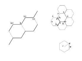
Figure 1: Graphene Lattice, BZ and One dimensional lattice on which the Harper equation is defined.

Now consider one Dirac fermion at the $K$-point with mass $m$ in magnetic field $B$. The Hamiltonian is $H=\sigma_{x}k_{x}+\sigma_{y}(k_{y}-eBx)+m\sigma_{z}$. For $eB>0$, the eigenstates are

$$u^{\pm}_{k,n}=\frac{e^{iky}}{4\pi\alpha_{n}}\left(\begin{array}[]{c}i\sqrt{\alpha_{n}\pm m}~{}\psi_{n}(x-x_{0}^{\pm}(k))\\ {}\hfil\\ \pm\sqrt{\alpha_{n}\mp m}~{}\psi_{n-1}(x-x_{0}^{\pm}(k))\end{array}\right)$$ (6)

with

$$\alpha_{n} = \sqrt{2|eB|n+m^{2}}$$

$$x_{0}^{\pm} = \frac{1}{eB}(k\pm\alpha_{n})$$

$$E^{\pm} = \pm\alpha_{n}$$

where $\psi_{n}(x)$ are harmonic oscillator eigenstates and $u^{\pm}$ are the eigenstates of $H_{K}$ with energies $E^{\pm}$. Notice that all the energy levels are paired except the $n=0$ level. There is a common misconception that unpaired “zero-modes” occur only for a massless fermion but observe that for $m>0$ we have $u^{-}_{k,0}=0$ while for $m<0$ we have $u^{+}_{k,0}=0$, so such levels are unpaired even for non-zero mass. In the field theory formalism, the current is defined to be $J^{\mu}=-\frac{1}{2}e\gamma^{\mu}_{\beta\alpha}[\psi_{\alpha},\overline{\psi}_{\beta}]$ and is odd w.r.t. charge conjugation symmetry. We find that

$$\langle 0|J^{0}|0\rangle=\rho=\frac{1}{2}(N_{-}-N_{+})\frac{|eB|}{2\pi}$$ (7)

where $N_{+}$ and $N_{-}$ are the numbers of filled positive and negative energy Landau levels (LL). Hence the Hall conductance is

$$\sigma_{xy}=\frac{1}{2}(N_{-}-N_{+})$$ (8)

in units of $e^{2}/h$. Due to the unpaired level, this will be half-integer and the position of the unpaired level depends on the sign of $eB$ and $m$ as in Fig[2].

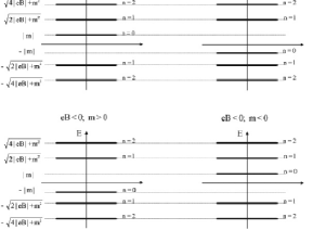
Figure 2: Zero mode in the Dirac Equation.

This analysis is correct for the fermion located around the $K$-point, but as mentioned before the graphene bandstructure contains two such fermions. For the purpose of being well defined, we consider a small positive Semenoff mass $m$ at $K$ which means a small negative mass at $K^{\prime}$. Consider the case of $eB>0$. The Hall conductance gets a contribution from both fermions and is zero when the Fermi level is in the gap $-m<\mu<m$ and odd integer otherwise. This is then an odd integer quantum Hall effect as in Fig[3]. When the gap is vanishingly small, $m\rightarrow 0$ the region of zero Hall conductance becomes infinitely narrow.

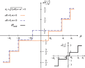
Figure 3: Hall conductance as a function of the chemical potential. The red and blue are the individual conductances from the two Dirac cones whereas the yellow one is the total Hall conductance.

II Harper Equation For Graphene

We now present a different argument that reproduces the experimental results and is valid for both high and low $B.$ The solution to this problem is to carefully examine the band structure and edge states of graphene in a magnetic field with rational flux $\phi=p/q.$ The analysis is based on a generalization of Hatsugai’s workHatsugai (1993a) to the honey-comb lattice. The energies of the bands and edge states are found as zeroes of certain polynomial equations. By using general polynomial theory we are able to characterize the bands, find the number of band crossings, and determine the conditions for zero modes and edge states. By identifying the Hall conductance as the winding index of the edge state around the band gap, we find that, as the magnetic field is decreased, the winding number of the edge states starts taking odd-integer values due to electron bands collapsing in pairs. The theoretical spectrum is obtained, and in addition, exact diagonalization results are presented to support it. It will be evident from the calculated bandstructure that for large magnetic fields the Dirac argument does not apply because the Hall conductances of bands at low-filling do not form a sequence of odd-integers in this case, as predicted by the relativistic argument.

We use the Landau gauge $A_{y}=Bx$, $A_{x}=0$, with $B=2\Phi/3\sqrt{3}a^{2}$, where $\Phi=p/q$ is the flux per plaquette (hexagon) and $p,q$ are relatively prime integers. With a Peierls substitution the effect of the magnetic field is $c_{i}^{\dagger}c_{j}\rightarrow c_{i}^{\dagger}c_{j}\exp{\int_{j}^{i}\vec{A}d\vec{r}}$. In this gauge $k_{y}=k$ is a good quantum number and the Hamiltonian for each $k$ is:

$$H(k)=-t\sum_{j}c_{k,2j-1}^{\dagger}c_{k,2j}A_{j}(k)+c_{k,2j}^{\dagger}c_{k,2j+1}+h.c.$$ (9)

where

$$A_{j}(k)=e^{i\pi\frac{p}{q}(j-\frac{5}{6})}+e^{-i\pi\frac{p}{q}(j-\frac{5}{6})}e^{ik}$$ (10)

Note that we have not included a mass term in our tight-binding Hamiltonian because graphene is essentially massless. Since $A_{j+q}=(-1)^{p}A_{j}$ the Hamiltonian is periodic with period $2q$, ($A_{j+2q}=A_{j}$) but the energy spectrum, which depends only on $|A_{j}|$ is periodic with period $q$. We start with the one-particle states $|\Psi(k,\phi)\rangle=\sum_{i}\psi_{i}(k,\phi)c^{\dagger}_{k,i}|0\rangle$ and act on these with the Hamiltonian to obtain the equation $H|\Psi\rangle=E|\Psi\rangle.$ There are two independent amplitude equations, one for $i$ odd and one for $i$ even:

$$\epsilon\psi_{2j-1}+A_{j}\psi_{2j}+\psi_{2j-2}=0$$

$$A_{j}^{\star}\psi_{2j-1}+\epsilon\psi_{2j}+\psi_{2j+1}=0$$ (11)

where $\epsilon=E/t$ with $E$ the energy. There are now two Harper equations for the hexagonal lattice, in contrast to the single Harper equation for the square lattice. After some manipulation we find in a transfer matrix formalism:

$$\left(\begin{array}[]{c}\psi_{2j+1}\\ \psi_{2j}\\ \end{array}\right)=\frac{1}{A_{j}}\tilde{M}_{j}\left(\begin{array}[]{c}\psi_{2j-1}\\ \psi_{2j-2}\\ \end{array}\right)$$ (12)

with

$$\tilde{M}_{j}=\left(\begin{array}[]{cc}\epsilon^{2}-A_{j}A_{j}^{\star}&\quad\quad\epsilon\\ {}\hfil\\ -\epsilon&-1\\ \end{array}\right).$$ (13)

As opposed to the transfer matrix for the square lattice, which hops by one site and is linear in energyHatsugai (1993a), the graphene transfer matrix hops by two sites and is quadratic in energy. This reflects the lattice periodicity. Since $\tilde{M}_{j+q}=\tilde{M}_{j}$, the periodicity of the energy spectrum is $q$. We can now define the transfer matrix over the magnetic unit cell:

$$M(\epsilon)=\left(\begin{array}[]{cc}M_{11}(\epsilon)&M_{12}(\epsilon)\\ M_{21}(\epsilon)&M_{22}(\epsilon)\\ \end{array}\right)\equiv\tilde{M}_{q}\tilde{M}_{q-1}...\tilde{M}_{1}.$$ (14)

By induction we find that $M_{11}$ is a polynomial of order $(\epsilon^{2})^{q}$, $M_{12}$ and $M_{21}$ are of the form $\epsilon\times(\epsilon^{2})^{q-1},$ while $M_{22}$ is a polynomial of order $(\epsilon^{2})^{q-1}$. These polynomials have coefficients which depend on $k$ and the magnetic flux. We pick our sample of order $L_{y}=2ql$, commensurate with the magnetic unit cell, where $l$ is a large integer and the factor of $2$ is added because we will require periodic conditions $\psi_{L_{y}}=\psi_{0}$, hence $L_{y}\equiv 0\equiv even$. The transfer matrix across the length of this sample is $M^{l}$. From HatsugaiHatsugai (1993a) we know that the important polynomial to consider is:

$$[M^{l}]_{21}(\epsilon)=0$$ (15)

The entire spectrum of energy levels for each $k$ value comes from the zeroes of this polynomial of which there are $L_{x}-1$. Some of these states are bulk states and others are edge states. We will now characterize the edge and bulk states (bands).

It is easy to find one solution to Eq.[15]. Simply take $M_{21}(\epsilon)=0$ and this will imply that Eq.[15]is satisfied since all upper-triangular matrices remain so when multiplied by another upper-triangular matrix. Hatsugai arguesHatsugai (1993a) that the energies of the edge states are given by the zeroes of exactly this polynomial: $M_{21}(\epsilon)=0$. Since $M_{21}(\epsilon)\sim\epsilon\times(a(\epsilon^{2})^{q-1}+b(\epsilon^{2})^{q-2}+\ldots),$ there is always one $\epsilon=0$ solution (zero mode edge state) which does not disperse and $2(q-1)$ non-zero energy solutions(edge-states) which come in pairs: $-\mu_{q-1}\leq-\mu_{q-2}\leq...\leq-\mu_{1}\leq 0\leq\mu_{1}\leq....\leq\mu_{q-2}\leq\mu_{q-1}$. Depending on whether $M_{11}(\mu_{i})/|A_{q}....A_{1}|$ is $<$,$>$, or $=1$ the edge state will be localized on the left edge, right edge, or be degenerate with the bulk i.e. touching a bulk stateHatsugai (1993a).

The bulk states are obtained from the lattice periodicity $j\rightarrow j+q$ and the Bloch condition:

$$\left(\begin{array}[]{c}\psi_{2q+1}\\ \psi_{2q}\\ \end{array}\right)=\rho(\epsilon)\left(\begin{array}[]{c}\psi_{1}\\ \psi_{0}\\ \end{array}\right)$$ (20)

with $\rho(\epsilon)$ a pure imaginary phase, i.e., $|\rho(\epsilon)|=1$. We also note that we have the transfer matrix equation

$$\left(\begin{array}[]{c}\psi_{2q+1}\\ \psi_{2q}\\ \end{array}\right)=\frac{1}{A_{q}A_{q-1}...A_{1}}M\left(\begin{array}[]{c}\psi_{1}\\ \psi_{0}\\ \end{array}\right).$$ (21)

Therefore, combining these two, $\rho(\epsilon)$ is an eigenvalue of the $2\times 2$ transfer matrix

$$\rho^{\pm}=\frac{1}{2A_{q}..A_{1}}[TrM\pm\sqrt{(TrM)^{2}-4|A_{q}....A_{1}|^{2}}].$$ (22)

where we have used $Det[M]=Det[M_{q}]...Det[M_{1}]=|A_{q}...A_{1}|^{2}$. It is easy to see that the Bloch condition $|\rho(\epsilon)|^{2}=1$ is satisfied for $(TrM)^{2}-4|A_{q}...A_{1}|^{2}<0$, based on the fact that $\rho^{+}\rho^{-}=1$. Since $M_{11}$ and $M_{22}$ are both polynomials of order $q$ in $\epsilon^{2}$ the solutions are again paired. Let us rewrite

$$(TrM(\epsilon^{2}))^{2}-4|A_{q}...A_{1}|^{2}=\prod_{i=1}^{2q}(\epsilon^{2}-\lambda_{i}),$$ (23)

with $0<\lambda_{1}\leq\lambda_{2}\leq\cdots\leq\lambda_{2q}$. The energy bands are thus

$$\begin{cases}\lambda_{2j+1}\leq\epsilon^{2}\leq\lambda_{2j+2}&\quad\text{bulk state}\\ ~{}\\ \lambda_{2j}\leq\epsilon^{2}\leq\lambda_{2j+1}&\quad\text{gap region}\end{cases}$$ (24)

for $j=0,1,\cdots,q-1$ and $\lambda_{0}=0$. The edge states lie in the gap region of the bulk band structure and the $\mu$’s are given by

$$\mu_{j}\in[\lambda_{2j},\lambda_{2j+1}]\quad j=1,\cdots,q-1.$$ (25)

We hence have $2q$ energy bands bounded by $4q$ $\lambda$’s, there are $2q-1$ gaps and $2q-1$ edge states as in Fig[4].

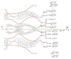
Figure 4: Schematic plot of the bulk band structure and edge states obtained from the transfer matrix formalism. Edge states are solid lines while bulk bands are denoted by the shaded areas bounded by dash and dotted lines.

Besides the above results of band structure, many more details about the spectrum can already be learned from the behavior of the function $|A_{q}A_{q-1}...A_{1}|(k)$,

1. The Hall conductance can be determined from the number of $k$’s that satisfy

   $M_{11}(\mu_{[j/2]})M_{22}(\mu_{[j/2]})=|A_{q}A_{q-1}...A_{1}|^{2}(k_{1})$.

2. The first bulk eigenvalue touches the zero energy edge state at the $k$ points where $|A_{q}...A_{1}|(k)=1$.

3. Bulk band width vanishes at $k$ if $|A_{q}...A_{1}|(k)=0$.

For graphene, $|A_{q}A_{q-1}...A_{1}|(k)$ can be explicitly written as

$$|A_{q}A_{q-1}...A_{1}|(k)=2^{q}\prod_{j=1}^{q}\left|\cos\left(\frac{k}{2}+\frac{(5-6j)p\pi}{6q}\right)\right|.$$ (26)

The periodicity of this function is $2\pi/q$. Hence the number of $k$’s at which $|A_{q}A_{q-1}...A_{1}|(k)=0$ is equal to $q$ while the number of $k$’s at which $|A_{q}A_{q-1}...A_{1}|(k)=1$ is equal to $2q$.

We shall now show how to obtain the details of the band structure from $|A_{q}A_{q-1}...A_{1}|(k)$. Let us assume that the edge state $\mu_{[j/2]}(k)$ touches the bulk at some point $k=k_{1}$

$$\mu_{[j/2]}(k_{1})=\epsilon_{j}(k_{1})=\pm\sqrt{\lambda_{j}(k_{1})}$$ (27)

where $[j/2]$ represents the largest integer less than or equal to $j/2$ and $j=1,...,2q$. Since $\epsilon_{j}(k_{1})$ is on the band edge, we have

$$M_{11}(\mu_{[j/2]})+M_{22}(\mu_{[j/2]})=\pm 2|A_{q}A_{q-1}...A_{1}|(k_{1}).$$ (28)

From the edge state condition $M_{21}(\mu_{[j/2]}(k_{1}))=0$, we also know

$$M_{11}(\mu_{[j/2]})M_{22}(\mu_{[j/2]})=|A_{q}A_{q-1}...A_{1}|^{2}(k_{1}).$$ (29)

We hence have

$$M_{11}(\mu_{[j/2]}(k_{1}))=M_{22}(\mu_{[j/2]}(k_{1}))=\pm|A_{q}...A_{1}|(k_{1})$$ (30)

when the edge state touches the bulk state. Thus, we can determine how many times the edge state starts from $\lambda_{2[j/2]}$ at $k_{1}$ and goes up in energy to touch $\lambda_{2[j/2]+1}$ at some $k_{2}$ then comes down again to touch $\lambda_{2[j/2]}$ at some $k_{3}$ etc. This defines the number of wrappings around the gap and represents the Hall conductanceHatsugai (1993a, b).

As a function of the momentum $k$ the first bulk eigenvalue $\lambda_{1}$ might touch the zero energy line (the zero mode) when $\epsilon_{1}(k)=0$. This happens when

$$M_{11}(0) = (-1)^{q}|A_{q}A_{q-1}...A_{1}|^{2};$$ (31)

$$M_{22}(0) = (-1)^{q};$$ (32)

$$M_{21}(0) = 0.$$ (33)

But from the previous analysis we know that when a bulk state touches an edge state $M_{22}=\pm|A_{q}...A_{1}|$. Hence the first bulk eigenvalue touches the zero energy edge state in $2q$ points in the first Brillouin zone, namely where $|A_{q}...A_{1}|=1$. This result is confirmed by our exact diagonalization, which will be presented later.

Using polynomial theory we can in fact prove a more stringent constraint. We separate the polynomial of order $2q$: $(TrM(\epsilon^{2}))^{2}-4|A_{q}...A_{1}|^{2}=(TrM(\epsilon^{2})-2|A_{q}...A_{1}|)(TrM(\epsilon^{2})+2|A_{q}...A_{1}|).$ Now, denote the eigenvalues of the two subfactors as $g$ for “green” and $b$ for “blue” respectively(for purpose of making the connection with the plots) and put them in ascending order:

$$TrM(\epsilon^{2})-2|A_{q}...A_{1}|=\prod_{j=1}^{q}(\epsilon^{2}-\lambda_{j}^{g}),$$

$$TrM(\epsilon^{2})+2|A_{q}...A_{1}|=\prod_{j=1}^{q}(\epsilon^{2}-\lambda_{j}^{b}),$$

where $\lambda_{1}^{g}<\lambda_{2}^{g}<...<\lambda_{q}^{g}$ and $\lambda_{1}^{b}<\lambda_{2}^{b}<...<\lambda_{q}^{b}$. (For $q=2$ the $<$ sign changes into $\leq$ due to the fact that in that case the system doesn’t break T and we can have gapless states.) Depending on whether $q$ is even or odd we have the following order:

$$q\;odd:\;\lambda_{1}^{b}\leq\lambda_{1}^{g}<\lambda_{2}^{g}\leq\lambda_{2}^{b}<...<\lambda_{q}^{b}\leq\lambda_{q}^{g}$$

$$q\;even:\;\lambda_{1}^{g}\leq\lambda_{1}^{b}<\lambda_{2}^{b}\leq\lambda_{2}^{g}<...<\lambda_{q}^{b}\leq\lambda_{q}^{g}$$ (34)

We can see that bulk states are between “blue” and “green” eigenvalues $|[\lambda^{b}_{i},\lambda^{g}_{i}]|,$ whereas the gaps are in between the consecutive “blue”-“blue” and “green”-“green” eigenvalues $|[\lambda^{g}_{i},\lambda^{g}_{i+1}]|$ or $|[\lambda^{b}_{i},\lambda^{b}_{i+1}]|$. As such, the width of a band is $|\sqrt{\lambda^{g}_{i}}-\sqrt{\lambda^{b}_{i}}|$. The band will become infinitely thin when $\lambda^{g}_{i}=\lambda^{b}_{i},$ or when $|A_{q}...A_{1}|=0$. This happens at $q$ points in the first Brillouin zone.

As an example, we can see everything above explicitly for the case $q=3,p=1$. There are $2q-1=5$ edge states with energies $-\mu_{2}(k),-\mu_{1}(k),0,\mu_{1}(k),\mu_{2}(k)$, where

$$\mu_{1,2}(k)=\sqrt{3+\cos{(k-\frac{7\pi}{9})}+\cos{(k-\frac{\pi}{9})}\mp\sqrt{\frac{5}{2}-\cos{(2k-\frac{8\pi}{9})}+\cos{(k-\frac{7\pi}{9})}(2+\cos{(k-\frac{7\pi}{9})})+(\cos{(k-\frac{7\pi}{9})})^{2}}}$$

There are $q=3$ points in the Brillouin zone where each band becomes infinitely thin given by

$$|A_{3}A_{2}A_{1}|(k)=0\;\;at\;\;k=\frac{4\pi}{9},\frac{10\pi}{9},\frac{16\pi}{9}.$$ (35)

The bands closest to zero energy touch the zero energy mode at $2q=6$ places in the Brillouin zone where

$$|A_{3}A_{2}A_{1}|(k)=1\;\;at\;\;k=\frac{\pi}{3},\frac{5\pi}{9},\pi,\frac{11\pi}{9},\frac{5\pi}{3},\frac{17\pi}{9}.$$ (36)

We also find that the condition $M_{11}(\mu_{1}(k))=M_{22}(\mu_{1}(k))$ is satisfied at two points in the Brillouin zone, which means that, in the first gap, the edge state touches the lower band $\lambda_{1}^{g}$ once and the upper band $\lambda^{g}_{2}$ also once, hence the Hall conductance is one. This is the same for when the Fermi level rests in the second gap, the condition $M_{11}(\mu_{1}(k))=M_{22}(\mu_{1}(k))$ being satisfied for two points in the Brillouin zone as well (see Fig[5]).

III Hall Conductance in Graphene

This section contains the theoretical results from the transfer matrix approach, as illustrated in the previous section, and the numerical results from exact diagonalization. The Hall conductance in graphene is defined, as usual, as the number of times the edge state wraps around the gap between neighboring energy bands. The number of left or right edge states that traverse the entire way across the gap is the Hall conductance. We then look at the evolution of the bands and edge states as the magnetic field is varied from very strong to weak. We will see how the edge states and band configuration for strong magnetic field, which do not match experiment, evolve into the weak-field limit, which does match the experiments.

This is accomplished in two ways: first, the “theoretical” edge states and band structure are found by numerically solving for the zeroes of the characteristic polynomials $M_{21}(\mu_{i})=0$ and $(TrM(\lambda^{g,b}_{i}))\pm 2|A_{q}...A_{1}|=0$ introduced in the previous section. We plot only the $\epsilon\geq 0$ states, the negative energy states being a mirror image. We also confirm the theoretical picture by exact numerical diagonalization of the Hamiltonian matrix for a relatively large number of lattice sites.

We start with $q=3$ in Fig[5]. We see that the Hall conductance is unity for a Fermi level in either the first or second gap, clearly in contradiction with the Dirac argument which would give $\sigma_{H}=1$ or $3$ depending on which gap. The number of bands is $2q=6$, there are $2q-1=5$ gaps and edge states, $q=3$ spots where each band becomes infinitely thin, and $2q=6$ points where the first band touches the zero energy mode.

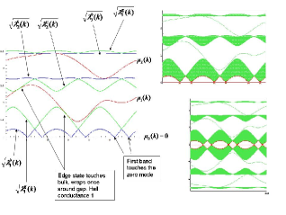
Figure 5: Left: Theoretical edge state and band structure configuration. The edge states are in red while the bulk bands are in between the consecutive blue and green lines ($\lambda^{b},\lambda^{g}$). The number of times an edge state wraps around the bulk is the Hall conductance, which in this case is unity $1$ for the both the first gap and the second gap. Right: The band structure obtained from direct diagonalization, upper right just the $\epsilon>0$ lower right is the full spectrum which is just a mirror image of the $\epsilon>0$ spectrum. From now on, we will plot only the positive energy part.

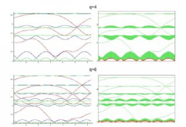
Figure 6: Left: Theoretical edge state and band structure configuration for $q=4$ and $q=6$. Right: Direct diagonalization.

We now continue by decreasing the magnetic field to $q=4$ and then $q=6$, see Fig[6]. For $q=4$ we have $\sigma_{xy}=1$ for a Fermi level in the first gap, $\sigma_{xy}=2$ for Fermi level in second gap, and $\sigma_{xy}=1$ for Fermi level in third gap. For $q=6$ the sequence is $\sigma_{xy}=1,4,3,2,1$ from the first to the fifth gap. This does not match the experimental observation of $\sigma_{xy}=1,3,5,7,etc.$

One crucial observation to notice is that, as we increase $q$ (decrease the magnetic field), the second and third bulk bands become closer and closer together in energy; the gap between them becomes smaller and smaller over the whole Brillouin zone. Eventually the second and third bands move entirely together upon increasing q (lowering B). For $q>12$, one cannot distinguish between the second and third band (nor can one distinguish the edge states between these bands). The second and third band have “collapsed” into a new band, a process which we call “band collapse.” After these bands have collapsed there are distinguishable gaps between the first band and the combined band, and then between the combined band and the fourth band. There are edge states between the top of the combined band and the fourth band, and these give $\sigma_{xy}=3$, for the Fermi level in what is now the second gap. If we then go to the next gap, this again does not match the experiment, with Hall conductance being $8.$

By increasing $q$ even further, we see that the fourth and fifth bands collapse in a similar fashion, and the gap between them vanishes uniformly across the $k$ spectrum as they become a single new band. This happens around $q=22$. The edge states between the collapsed second and third bands and the collapsed fourth and fifth bands remain the same as before, giving $\sigma_{xy}=3$ but now the edge states between the collapsed fourth and fifth bands and the sixth band give $\sigma_{xy}=5$. This process repeats itself while $q$ is increased. The total number of bands increases when $q$ is increased. But some of these bands collapse together so that we cannot distinguish them unless we have infinite resolution. We present the results for $q=31$ Fig[8].

Upon increasing $q$ the band collapse leads to double degeneracy of each of the bands except the zero energy band, and this gives the odd integer Hall conductance in graphene. This is beautifully seen as the number of positive or negative-slope edge states that disperse in the resolvable gaps. Hence the experimental situation is theoretically confirmed as the weak-field limit of graphene.

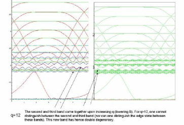
Figure 7: Left: Theoretical edge state and band structure configuration for $q=12$. Right: Direct diagonalization.

The theoretical band structure can actually be continued to large $q$, as the polynomials are well behaved. We give the $q=49$ plot as well, where we can see all the odd-integer quantum hall effects from $1,3,5,7,9,11,$ see Fig[9].

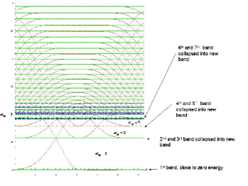
Figure 8: Left: Theoretical edge state and band structure configuration for $q=31$.

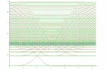
Figure 9: Left: Theoretical edge state and band structure configuration for $q=49$.

By examining the common properties of each bandstructure plot it appears that the spectrum of bands and edge-states can be classified into two parts: a relativistic section and a non-relativistic section. This structure originates from the original tight-binding dispersion relations without the B field,

$$\epsilon(k_{x},k_{y})=\pm t\sqrt{1+4\cos^{2}\frac{\sqrt{3}}{2}k_{x}+4\cos\frac{\sqrt{3}}{2}k_{x}\cos\frac{3}{2}k_{y}}.$$

The Dirac nodes are located at $(\pm\frac{4\pi}{3\sqrt{3}},0)$ and $(\pm\frac{2\pi}{3\sqrt{3}},\pm\frac{2\pi}{3})$. The linearized dispersion relations persist up to around $E\approx t$. Above this energy scale the bands become parabolic. Accordingly, in Fig. 9, $\sigma_{xy}=1,3,5$ … at low energy and the energy of bulk levels goes as $E_{n}\approx\sqrt{n},$ a feature of relativistic Landau levels. On the other hand $\sigma_{xy}=1,2,3,....$ starting from the top of the bands (where parabolic bandstructure is expected) and there is almost equal spacing between each of these Landau levels, which is a feature of the harmonic-oscillator-like non-relativistic Landau levels. A $\sigma_{xy}$ of $1$ is seen in the first gap from the band ceiling and increases by one for each Landau level below the top. A similar thing occurs for the non-relativistic levels near the bottom of the set of bands. The crossover region is at $E\approx t,$ where the band collapse occurs.

The odd-integer sequence shown in Fig[9] is clearly represented in the experimental data which, as stated before, is in the low magnetic field limit of graphene. With a flux $\phi=1/q$ in each unit cell the magnetic field is $\sim\frac{1.3\times 10^{5}}{q}\;\;\rm{Tesla}$ which is a very large magnetic field. For experimentally realizable magnetic fields we would expect $q\sim 1000$ and the odd-integer sequence would be continued to larger values. Abnormalities in this sequence would not arise until more Landau levels were filled. Overall, there will be a sequence (possibly very long) of odd-integer quantum Hall conductances followed by conductances which do not follow a certain pattern. Then there will be a relativistic-non-relativistic crossover region where the Landau level spacings change character from $n^{1/2}$ to $n$. The non-relativistic energy levels will then persist to higher energies.

III.1 Effect of Disorder

We have considered the stability of the edge-states under disorder. Although not tractable analytically, we were able to use numerical diagonalization (which up to now has remarkably matched the analytic results) to study the introduction of disorder into the system. The disorder term we added to the system is:

$$H_{dis}(k)=X_{D}\delta_{IJ}$$ (38)

where $X_{D}$ is a random variable with gaussian distribution and mean $0,$ and $I,J=1,2,\ldots L-2,L-1.$ We also tested a uniform distribution for the $X_{D}$ with essentially the same results. For relatively high disorder e.g. the variance of $X_{D}\sim 0.15$ the structure of the lowest energy edge state is robust (see Fig[10]). However, the edge states representing higher plateaus, such as $n=3,5,7,9,11,\ldots$ are washed out. Note that the hopping parameter is defined to be $1,$ so $0.15$ is very high disorder. For lower disorder, with the variance of $X_{D}\sim 0.01,$ all of the edge states are clearly visible up to the relativistic-non-relativistic crossover (see Fig[11]), just as in the disorder-free plots given above; e.g. as in Fig[7].

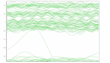
Figure 10: Numerical calculation for edge states and band structure for $q=10$ and disorder variance $0.15.$

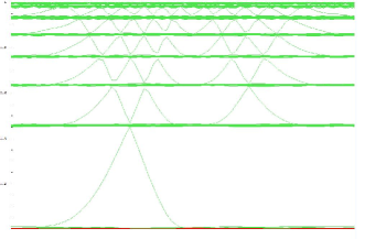
Figure 11: Numerical calculation for edge states and band structure for $q=50$ and disorder variance $0.01.$

III.2 Non-zero Semenoff term

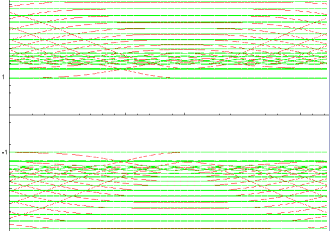
Figure 12: (color online) (a)Theoretical edge state and band structure configuration for $q=17$, with Semenoff mass $m=1.$

The previous formalism can be easily extended to incorporate the case of a non-zero Semenoff mass $m$. As an example, for Boron Nitride (BN) the hamiltonian has the form:

$$H=-t\sum_{j}((c_{2j-1}^{\dagger}c_{2j}A_{j}+c_{2j}^{\dagger}c_{2j+1}+h.c.)$$

$$+m(c_{2j-1}^{\dagger}c_{2j-1}-c_{2j}^{\dagger}c_{2j}))$$ (39)

The new Harper’s equations are:

$$(\epsilon+m)\psi_{2j-1}+A_{j}\psi_{2j}+\psi_{2j-2}=0$$

$$A_{j}^{\star}\psi_{2j-1}+(\epsilon-m)\psi_{2j}+\psi_{2j+1}=0$$ (40)

and the transfer matrix now becomes:

$$\tilde{M}_{j}=\left(\begin{array}[]{cc}\epsilon^{2}-m^{2}-A_{j}A_{j}^{\star}&\epsilon-m\\ -(\epsilon+m)&-1\\ \end{array}\right)$$ (41)

As we can see, $\tilde{M}_{q}\tilde{M}_{q-1}....\tilde{M}_{1}=(\epsilon+m)\times P^{(q-1)}(\epsilon^{2})$ where $P^{(q-1)}(\epsilon^{2})$ is a polynomial of order $q-1$ in $\epsilon^{2}$. Hence the former zero energy edge state has now moved to $\mu_{0}=-m$. There are no edge states between $[-|m|,+|m|]$, but the rest of the analysis applies. We plot the band structure for $m=1$, $q=17$ (see Fig[12]).

IV Spin and Valley Splitting in the $n=0$ Landau Level

$\begin{array}[]{c}\begin{@subfigure}\includegraphics[scale={0.34}]{spingap.eps}\end{@subfigure}\\ \begin{@subfigure}\includegraphics[scale={0.35}]{massgap.eps}\end{@subfigure}\\ \begin{@subfigure}\includegraphics[scale={0.35}]{spinandmassgap.eps}\end{@subfigure}\end{array}$

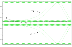
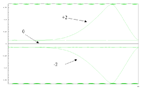
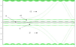
Figure 13: Landau level bands and edge states around E=0 for (a)Spin splitting only (b)Valley splitting only (c) Spin and valley splitting. Quantum Hall conductances for particular gaps are noted by the integer labels and are in units of $e^{2}/h.$

We now focus on the breaking of spin and/or valley degeneracy in the $n=0$ Landau Level. The idea of spin splitting is very natural since $g\sim 2$ in graphene and there is a large magnetic field applied perpendicular to the sample. Splitting the valleys however, is more subtle since there is no natural alternating sublattice potential or applied strain. We investigate the changes to the QHE plateau structure and edge states when these splittings can be resolved energetically.

First we consider the case of only spin splitting. Due to the Zeeman effect the spin states in each Landau level will be split by $g\mu_{B}B.$ For the $n=0$ Landau level one spin state is pushed above zero energy and the other is pushed below zero energy. When the chemical potential lies in the gap at zero energy between the split spin states there is an additional QH plateau with $\sigma_{xy}=0.$ The picture is not quite this simple because this gap, unlike the Semenoff mass gap discussed above, contains edge states which can be seen in Fig[13]Abanin et al. . Usually the presence of edge states in the gap signals a non-zero QH conductance but here there is actually one electron edge state and one hole edge state. These two edge states combine together to give zero Hall conductance but produce a non-zero spin-Hall conductivity since they are spin-polarized in opposite directions:

$$\sigma_{spin}=2\frac{e^{2}}{\hbar}.$$ (42)

This spin current can be observed in a $4$-terminal geometry or in a system with magnetic leads.

The case where only the valleys are split in the $n=0$ level, no matter by what means, is very similar to the case of a non-zero Semenoff mass given above. As in that case there is a gap at zero energy leading to an additional zero conductance plateau, however here there are no edge states in the gap, thus no spin Hall conductivity. The band picture and sequence of quantum Hall conductances can be seen in Fig[13].

Finally we come to the case where there are both spin and valley splittings. Gaps will appear when the $n=0$ level is unfilled, $1/4$-filled,$1/2$-filled, $3/4$-filled, and completely filled yielding a sequence of QH conductances $\sigma_{xy}=-2,-1,0,1,2$ in units of $e^{2}/h$ when the chemical potential lies in each of these gaps. The band picture with each of these conductances can be seen in Fig[13]. This sequence matches the data recently produced by Zhang et al. in very high magnetic fields.In the graphene sample there will be some small valley splitting due to imperfections (shear strain, impurities, or surface roughness) but not enough to produce a gap large enough to exhibit the quantum Hall effect. Since there is no applied strain we must look for many-body effects that would give rise to this splitting.

The idea of exchange ferromagnetism, which applies in the non-relativistic quantum Hall effect is also applicable here with some differences. In a normal QH system we expect that for the lowest Landau level we should see valley-polarized ground statesM et al. (1985); Rasolt et al. (1986). The $\sqrt{n}$ dependence in the graphene Landau level spectrum should not be important as long as the Landau gap is large i.e. $\hbar\omega_{c}>>e^{2}/\ell_{B},\hbar/\tau.$ The excitation energy of skyrmions has been calculated in Kallin and Halperin (1984). However, if we considered higher Landau levels there would be some quantitative corrections.

The second thing to consider is the correlation between the valley index and the sublattice index. For the $n=0$ level if an electron is in a particular valley then its spatial wavefunction resides on a single sublattice, A or B. If this Landau level is $1/4$-filled or $3/4$-filled there will be a valley and spin polarized ground state. The spin polarization is from the Zeeman splitting and the system will form a valley-polarized “ferromagnet”-like state due to exchange correlations. In this level the valley and sublattice are correlated, but they are correlated such that if the electrons reside in only one valley then they reside on a single sublattice which minimizes the Coulomb interaction. This leads to a spin-polarized charge modulation where there will be an excess of charge on one sublattice. This will form a weak charge density wave with charge density modulation where the percentage of charge modulation is proportional to $N_{0}/N_{T}$, the amount of electrons in the $n=0$ Landau level divided by the total number of electrons in the system. The electrons that participate in the charge modulation are effectively the difference between the number of electrons at half-filling and the number of electrons currently in the system.

This valley polarized ground state will produce an interaction gap characterized by the energy to produce a charged excitation. Since there is no applied strain we expect that $SU(2)$ valley skyrmions will be cheaper to create than particle-hole excitations Sondhi et al. (1993). We do not expect to see full $SU(4)$ skyrmions because the $g$-factor in graphene is not smallSondhi et al. (1993). This raises the possibility of measuring valley skyrmions in graphene as was recently done in AlGaAs Y. P. Shkolnikov et. al. (2005). Since we are projecting into the $n=0$ Landau level we can use the calculation of Kallin and Halperin (1984); Arovas et al. (1999) to estimate the spin stiffness and thus give an estimate of the energy to create a skyrmion: $E_{sk}=4\pi\rho_{s}=\frac{1}{4}\sqrt{\pi/2}(e^{2}/\epsilon\ell_{B}).$ If we compare the energy width of the plateau of the spin-split states to that of the valley-split states shown in Zhang et al. they are roughly of the same order of magnitude. However $E_{sk}/(g\mu_{B}B)\sim 54$ at $B=45T$ so our skyrmion energy is clearly an overestimate. For the valley skyrmions measured in AlGaAsY. P. Shkolnikov et. al. (2005) the data also clearly shows that $E_{sk}$ is an overestimate by a factor of $\sim 40$ for their systems at zero applied strain. This factor compensates for the overestimation and brings the skyrmion energy to the right order of magnitude. Another interesting fact is that at low magnetic field this valley splitting gap vanishes and the $\sigma_{xy}=\pm 1$ plateaus disappear. This could be the result of there being two few electrons in the $n=0$ Landau level to produce this well correlated effect. Overall the valley degeneracy splitting suggests that small spin-polarized charge density modulation or valley skyrmions could be measured in graphene.

V Conclusion

We have shown that the “relativistic” quantum Hall effect in graphene has its origin in a band-collapse picture where two bands become degenerate upon decreasing the flux per plaquette. A series of exact results for the honeycomb lattice are given, as well as an index theorem for the number of dirac modes in a magnetic field. At large magnetic fields, the system has a transition between “relativistic” and non-relativistic QHE. When the spin-gap is resolved, the system exhibits a spin-Hall effect due to existence of opposite spin electron and hole edge states in the gap. We discussed the effects of disorder and adding a Semenoff mass term. We concluded with discussion on spin and valley splitting in the $n=0$ Landau level and its implications for the quantum Hall effect.

VI Note

During the preparation of this paper, we have noticed a series of other papers that have independently reached some of the conclusions presented in this manuscriptAbanin et al. ; Nomura and MacDonald ; Fertig and Brey ; Yang et al. ; Hatsugai et al. .

VII Acknowledgements

B.A.B acknowledges support from the SGF. T.L.H. acknowledges support from NSF. This work is supported by the NSF under grant numbers DMR-0342832 and the US department of Energy, Office of Basic Energy Sciences under contract DE-AC03-76SF00515.

References

- K. S. Novoselov et. al. (unpublished) K. S. Novoselov et. al., Nature 438, 197 (2005).
- Y. Zhang et. al. (unpublished) Y. Zhang et. al., Nature 438, 201 (2005).
- Wallace (1947) P. R. Wallace, Phys. Rev. 71, 622 (1947).
- Semenoff (1984) G. W. Semenoff, Phys. Rev. Lett. 53, 2449 (1984).
- Haldane (1988) F. D. M. Haldane, Phys. Rev. Lett. 61, 2015 (1988).
- Schakel (1991) A. M. Schakel, Phys. Rev. D 43, 1428 (1991).
- Peres et al. (2006) N. M. R. Peres, F. Guinea, and A. H. C. Neto, Phys. Rev. B 73, 125411 (2006).
- Gusynin and Sharapov (2005) V. P. Gusynin and S. G. Sharapov, Phys. Rev. Lett. 95, 146801 (2005).
- Kane and Mele (2005a) C. I. Kane and E. J. Mele, Phys. Rev. Lett. 95, 226801 (2005a).
- Kane and Mele (2005b) C. I. Kane and E. J. Mele, Phys. Rev. Lett. 95, 146802 (2005b).
- (11) Y. Yao, F. Ye, X.-L. Qi, S.-C. Zhang, and Z. Fang, cond-mat/0606350.
- (12) H. Min, J. Hill, N. Sinitsyn, B. Sahu, L. Kleinman, and A. MacDonald, cond-mat/0606504.
- Jackiw and Rebbi (1976) R. Jackiw and C. Rebbi, Phys. Rev. D 13, 3398 (1976).
- Hatsugai (1993a) Y. Hatsugai, Phys. Rev. B 48, 11851 (1993a).
- Hatsugai (1993b) Y. Hatsugai, Phys. Rev. Lett. 71, 3697 (1993b).
- (16) D. A. Abanin, P. A. Lee, and L. S. Levitov, cond-mat/0602645.
- (17) Y. Zhang, Z. Jiang, J. P. Small, M. S. Purewal, Y.-W. Tan, M. Fazlollahi, J. D. Chudow, J. A. Jaszczak, H. L. Stormer, and P. Kim, cond-mat/0602649.
- Kallin and Halperin (1984) C. Kallin and B. I. Halperin, Phys. Rev. B 30, 5655 (1984).
- M et al. (1985) R. M, F. Perrot, and A. H. MacDonald, Phys. Rev. Lett. 55, 433 (1985).
- Rasolt et al. (1986) M. Rasolt, B. I. Halperin, and D. Vanderbilt, Phys. Rev. Lett. 57, 126 (1986).
- Sondhi et al. (1993) S. L. Sondhi, A. Karlhede, S. A. Kivelson, and E. H. Rezayi, Phys. Rev. B 47, 16419 (1993).
- Y. P. Shkolnikov et. al. (2005) Y. P. Shkolnikov et. al., Phys. Rev. Lett. 95, 066809 (2005).
- Arovas et al. (1999) D. P. Arovas, A. Karlhede, and D. LillieHook, Phys. Rev. B 59, 13147 (1999).
- (24) K. Nomura and A. H. MacDonald, cond-mat/0604113.
- (25) H. Fertig and L. Brey, cond-mat/0604260.
- (26) K. Yang, S. D. Sarma, and A. H. MacDonald,cond-mat/0606504.
- (27) Y. Hatsugai, T. Fukui, and H. Aoki,cond-mat/0607669.