To knot or not to knot

Abstract

We study the formation of knots on a macroscopic ball-chain, which is shaken on a horizontal plate at 12 times the acceleration of gravity. We find that above a certain critical length, the knotting probability is independent of chain length, while the time to shake out a knot increases rapidly with chain length. The probability if finding a knot after a certain time is the result of the balance of these two processes. In particular, the knotting probability tends to a constant for long chains.

I Introduction

Knots are prevalent on most cables, chains, and strings being used in every day life or technology. Most remarkably, knots appear to form spontaneously, as soon as strings are shaken, transported, or handled in any way, and thus are an unavoidable byproduct of their use. For example, B01 describe the dynamics of a ball chain that is suspended from an oscillating support. As soon as the chain dynamics become chaotic, the chain forms knots of various kinds. Yet in spite of a considerable amount of work on the importance of knots on the molecular scale WC86 ; KM91 , we are not aware of any systematic study into the origin of the prevalence of knots on macroscopic chains.

In this paper we present model experiments on shaken ball chains that quantify the tendency for knot formation as function of chain length. By considering both knotting and unknotting events, we present a simple theory that explains the probability for the formation of knots after the chain has been shaken for a given amount of time. After the experiment, the ends of the chain lie flat on the plate, and there is a unique way to join the ends to form a closed curve. If this curve is topologically equivalent to a closed loop or “unknot” A00 there is no knot, otherwise we call the chain knotted. We made no distinction between different kinds of knots, however the simple trefoil knot A00 was by far the most common.

Of course, it is precisely the topological stability of knots that lies at the root of the phenomenon: once a knot is created, it cannot disappear, except when it falls out at the end of the chain. Using a setup very similar to ours, the pioneering study BDVE01 investigated the lifetime of a simple trefoil knot that was placed in the middle of the chain at the beginning of the experiment. The mean lifetime $\tau$ of the knot was found to increase rapidly with chain length:

$$\tau=\tau_{3}(N-N_{0})^{2}/D,$$ (1)

where N is the number of balls on a chain, $N_{0}\approx 15$ the size of a knot, and $D$ a hopping rate. The knot was modeled by the three points of intersection of the chain, which perform random walks. From this assumption the constant $\tau_{3}=0.056213$, as well as the entire distribution of lifetimes was calculated. The experimentally determined hopping rate of $D=11\pm 1s^{-1}$ was found to be close to the driving frequency of $f=13Hz$; however, it has not been investigated systematically what sets this time scale.

In Fig. 1 we present a sketch of our experimental setup. A stiff solid plate, 50 cm in diameter, is vibrated vertically by an electrodynamic shaker. The plate’s weight of 4 kg is sufficiently large for the chains to have little effect on the motion of the plate.

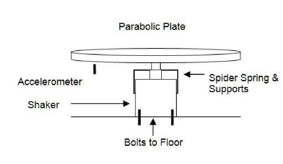
Figure 1: Sketch of the experimental setup.

The plate is attached to a metal block mounted on a spider spring, to support the weight of the plate and to reduce lateral motion. The shaker is controlled by a computer, with an accelerometer providing feedback to make sure the plate motion is close to sinusoidal. The driving frequency $f=21Hz$ is dictated by the requirement of operating close to resonance, the dimensionless acceleration is $\Gamma=A\omega^{2}/g=12\pm 0.2$ as recorded by the accelerometer. Here $A$ is the amplitude, $\omega=2\pi f$ the angular frequency, and $g$ the acceleration of gravity. The top of the plate was machined to have a very shallow parabolic profile, of 5mm depth at the center of the plate. This amount of confinement was enough to always keep the chains near the center, without them ever feeling the edge of the plate. A digital camera was mounted above the plate, capable of taking up to 20 frames per second.

Ball chains are an excellent model system to study knot formation BDVE01 , in that they have little stiffness that would resist the formation of loops, yet considerable friction between the beads keeps knots from opening too easily. All our chains were cut from a single sample that had a bead diameter of $2R_{bead}=2.1\pm 0.05mm$, with connecting rods that allowed for a maximum inter-bead spacing of $2.1\pm 0.05mm=2R_{bead}$, somewhat greater than that of the earlier study ($0.8R_{bead}$) BDVE01 . It seems reasonable to take the number of beads as the fundamental unit of length, since they offer the greatest resistance as two parts of the chain slide across each other.

II Experimental results

Our main aim is to understand and to quantify the tendency for knots to form spontaneously once excited by shaking. To that end we shake chains of lengths between N=10 and 500 by dropping them onto the vibrating plate, and inspecting them for knots after 30 seconds. Each experiment was repeated 80 times, and the resulting probability of knotting calculated, as shown in Fig. 2. No knotting was ever observed for chains shorter than $N_{min}=38$. The probability then rises sharply to reach a plateau value of about $P=0.26$.

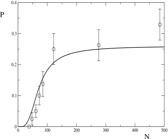
Figure 2: Probability for knotting after 30 seconds. Error bars are calculated from the variance of a binomial distribution. The full line is based on equation (3) below.

We expect that Fig. 2 can be understood from the interplay of knotting and unknotting events. To investigate this further, we followed the evolution of chains whose length lay in the transition region (N=73 and N=144) continuously for two hours. By taking 10 frames at 20 fps we were able to decide unambiguously whether a knot was present. This process was repeated every 5.5 seconds, which permitted us to compress and store the video images. The entire sequence was then examined manually for the number of knots, separated by a length of chain. As shown in Fig. 3, the presence of two knots is still quite unlikely for the chain lengths shown here. In calculating the statistics of knotting and unknotting, knots were treated as independent.

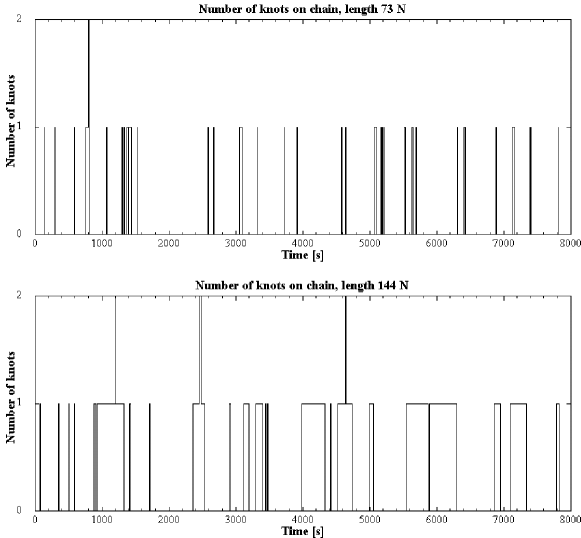
Figure 3: The number of knots on chains of length N=73 and N=144 as a function of time.

Some statistics as extracted from Fig.3 are collected in Table 1. As expected, the lifetime of a knot increases considerably with length. Comparing to the results of BDVE01 , there is remarkably good agreement, using (1) with the same value of the hopping rate $D$ as in the original paper. This is perhaps surprising, considering the differences in chain properties, driving conditions and, in particular, in the way knots are introduced. In BDVE01 , knots were introduced by hand in the center of the chain, while spontaneous knots tend to originate from the end of the chain, see Fig. 4 below. Note that our driving frequency was also somewhat larger than that of BDVE01 .

Chain length [N]	73	144
Chain length [cm]	30	60
mean knot lifetime [s]	$13\pm 5$	$102\pm 29$
$\tau$ [s] BDVE01	17	85
mean knotting time [s]	$219\pm 12$	$219\pm 16$
$<R_{g}>$ [cm] (no knot)	$7.18\pm 0.03$	$11.58\pm 0.06$
$<R_{g}>$ [cm] (knot)	$6.39\pm 0.12$	$11.00\pm 0.09$

Table 1: Some statistics of knotting and unknotting for two chains, N=73 and N=144. The last two lines report the mean radius of gyration.

However the most remarkable observation is that the mean knotting time for the two chains is the same, although the chain lengths are quite different. This observation makes sense, since knots are produced by the ends of the chain, which have sufficient freedom of motion to wrap around the rest of the chain, as illustrated by the three knotting events shown in Fig. 4. Of course, there is certain minimum length that is required, which according to Fig. 2 is $N_{min}=38$, about twice the minimum size $N_{0}$ of a knot. Our data for $N=73$ indicates that the knotting rate rises very quickly to a plateau value in the chain length. We will assume that the knotting rate is actually constant once $N$ is larger than $N_{min}$.

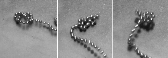
Figure 4: Examples of knotting events, taking place at the end of the chain.

In Fig. 5, we plotted the cumulative distribution of knotting times for the shorter chain, as obtained from the data of Fig. 3. The result is very well fitted by an exponential distribution, using the mean knotting time $\tau_{k}$ from Table 1. This is the distribution we will assume below for both knotting and unknotting events, although the unknotting distribution is more complicated BDVE01 .

\psfrag{N}{\large$K$}\psfrag{t}{\large$t[s]$}\psfrag{n1}{\large$K=K_{tot}(1-\exp(-t/\tau_{k}))$}\psfrag{n2}{\large$\tau_{k}=219s$}\includegraphics[width=303.53267pt]{total1.eps}

Figure 5: Cumulative number $K$ of knotting events occurring after a shaking time of $t$ or smaller.

As a final result, we report the mean radius of gyration $<R_{g}>$ obtained by taking the spatial average of all beads of a chain, which was done by image analysis using MATLAB. We then performed a temporal average, which we did separately for the knotted and the unknotted chain. As expected, $<R_{g}>$ is slightly larger for the unknotted state, but temporal fluctuations are prohibitively large to make this a useful indicator of knottedness, as we had hoped originally. The radius of gyration of course increases with chain length, but at a slower rate than the linear extension of the chain.

III Theory and Discussion

Armed with the above observations, we can attempt a simple theory for the probability of knots. We adopt a two-state description, in which the chain is either in an unknotted or in a knotted state, the probability of the latter being $P$. This can easily be generalized to allow for an arbitrary number of knots. Events are completely uncorrelated in time, so the distribution of (say) unknotting times is assumed exponential, while reality is more complicated BDVE01 . Now if the average unknotting time is $\tau$ as before, and the knotting time $\tau_{k}$, we obtain the following rate equation for $P$:

$$\dot{P}=(1-P)/\tau_{k}+P/\tau.$$ (2)

The first term is the rate of knotting events, which only take place if there is no knot. Conversely, the second term describes the rate of unknotting. Equation (2) is solved very simply with initial condition $P(0)=0$, giving

$$P(t)=\frac{1}{1+\tau_{k}/\tau}\left[1-\exp(-(\tau^{-1}+\tau_{k}^{-1})t)\right].$$ (3)

for the probability after a time $t$. Now all that is needed are the values of $\tau$ and $\tau_{k}$ as function of chain length.

For $\tau$ we take (1) as found in BDVE01 , which according to Table 1 is consistent with our data. For the knotting time we take

$$\tau_{k}=\left\{\begin{array}[]{lcl}\infty&&N<=N_{min}\\ \tau_{k}^{(sat)}&&N>N_{min}\\ \end{array}\right..$$ (4)

As discussed above, this is based on the idea that knots are formed at the end of the chain. Once a length $N_{min}$, which gives sufficient freedom for knots to form, is exceeded, the rest of the chain no longer matters. By the same argument we also believe that the mean configuration of the chain, as measured qualitatively by the radius of gyration, is not of fundamental importance to calculate knotting probabilities. The constant $\tau_{k}^{(sat)}$ has to be determined empirically.

For long chain lengths, $\tau$ becomes large and (3) reduces to $P=1-\exp(-t/\tau_{k}^{(sat)})$, independent of chain length, as expected. From the asymptotic value of $P=0.26$, taken from Fig. 2, we deduce $\tau_{k}=100s$. For simplicity, we also assume that $N_{min}$ is essentially the same quantity as $N_{0}$ as identified by BDVE01 , the length for which a knot falls out immediately. The result, (3), is plotted as the solid line in Fig. 2, using (1),(4). The agreement is quite good, considering there is only one adjustable parameter.

Ideally, even this adjustment could have been avoided, as $\tau_{k}$ could be taken directly from Table 1. However, this gives about twice the value of $\tau_{k}$, which would lead to a significant disagreement in the asymptote of $P$. One simplifying assumptions of our model was to disregard the distribution of knotting times. However we suspect that the main reason for this disagreement lies in the difficulty of preparing the chain in an unbiased fashion. At the beginning the ends of the chain are excited to a higher degree, leading to a significant increase of the knotting probability.

There is a significant body of work that remains to be done. Firstly, one would like to check our theory in greater detail, by taking long time traces for a greater variety of chain lengths, and measuring knotting probabilities for periods other than 30 s. Secondly, one would like to obtain a better description of the dynamics of the chain, and how it leads to knotting events. In particular, what sets the time scale for $\tau$ and $\tau_{k}$ ? This could be addressed in part by changing the driving characteristics of the plate, as well as the amount of confinement of the chain. Preliminary experiments, performed in a container with side walls, have in fact shown that boundary effects play a significant role for the knotting probability. Finally, we have not considered the probability for different types of knots, which are observed if the knotting time increases.

- (1) A. Belmonte et al. Phys. Rev. Lett. 87, 114301 (2001).
- (2) S. A. Wasserman and N. R. Cozzarelli, Science 232, 951 (186).
- (3) K. Koniaris and M. Muthukumar, Phys. Rev. Lett. 66, 2211 (1991).
- (4) A. C. Adams, The Knot Book, Freeman (2000).
- (5) E. Ben-Naim et al., Phys. Rev. Lett. 86, 1414 (2001).