Electrostatic interactions across a charged lipid bilayer

Abstract

We present theoretical work in which the degree of electrostatic coupling across a charged lipid bilayer in aqueous solution is analyzed on the basis of nonlinear Poisson-Boltzmann theory. In particular, we consider the electrostatic interaction of a single, large macroion with the two apposed leaflets of an oppositely charged lipid bilayer where the macroion is allowed to optimize its distance to the membrane. Three regimes are identified: a weak and a high macroion charge regime, separated by a regime of close macroion-membrane contact for intermediate charge densities. The corresponding free energies are used to estimate the degree of electrostatic coupling in a lamellar cationic lipid-DNA complex. That is, we calculate to what extent the one-dimensional DNA arrays in a sandwich-like lipoplex interact across the cationic membranes. We find that, in spite of the low dielectric constant inside a lipid membranes, there can be a significant electrostatic contribution to the experimentally observed cross-bilayer orientational ordering of the DNA arrays. Our approximate analytical model is complemented and supported by numerical calculations of the electrostatic potentials and free energies of the lamellar lipoplex geometry. To this end, we solve the nonlinear Poisson-Boltzmann equation within a unit cell of the lamellar lipoplex using a new lattice Boltzmann method.

Introduction

Lipids self-assemble in aqueous solution into a variety of morphologically different structures among which the planar bilayer is the biologically most relevant one. Almost all naturally occurring lipid membranes contain to some degree acidic lipids which forms the basis for electrostatically-driven protein adsorption. In fact, the adsorption of macroions onto oppositely charged lipid membranes is an ubiquitous phenomenon not only in the living cell but is also common in technological and pharmaceutical applications [Evans and Wennerström, 1994]. For example, the formation of cationic lipid-DNA complexes [de Lima et al., 2001]– one of the most promising carriers for non-viral gene delivery – is based on electrostatic interactions and subsequent complexation of cationic lipids and (the negatively charged) DNA.

What determines the electrostatic properties of a lipid bilayer is not only the mole fractions (and valencies) of the charged lipid species but also the low dielectric constant of the membrane interior [Israelachvili, 1992]. The large drop in the dielectric constant across a lipid bilayer makes it energetically unfavorable for large electric fields to form and thus dramatically diminishes the electrostatic coupling between the two charged monolayers of a lipid bilayer. Similarly, the electrostatic interaction between two charged macroions, adsorbed on the opposite leaflets of a lipid bilayer, is masked.

We mention two systems where the electrostatic interaction across a lipid bilayer may be significantly enhanced: The first concerns the deposition near a lipid membrane of an anorganic crystal, calcium pyrophosphate dihydrate, leading to crystal-induced membranolysis. A recent Molecular Dynamics simulation of crystal deposition on the zwitterionic membrane dimyristoylphosphatiadylcholine (DMPC) suggests that membrane rupture starts in the apposed monolayer and is induced by electrostatic interactions across the bilayer [Dalal et al., 2006]. The second system is the lamellar cationic lipid-DNA complex structure [Rädler et al., 1997, Lasic et al., 1997] (also referred to as lipoplex or $L_{\alpha}^{C}$ phase; see below in Fig. 4 for a schematic representation) which consists of a lamellar bilayer stack with one-dimensional arrays of DNA intercalated. Experimental evidence suggests that the DNA arrays in different galleries are orientationally ordered [Battersby et al., 1998], implying the presence of DNA-DNA interactions across the membrane. Previous theoretical modeling of this observation was based on the assumption that this coupling is mediated through elastic [Harries et al., 2003] or electrostatic [Schiessel and Aranda-Espinoza, 2001] interactions. In the latter study, however, it was assumed that the membrane is infinitely thin, thus neglecting the presence of regions with low dielectric constant. Whether direct electrostatic DNA-DNA interaction may lead to the coupling is thus still an open question.

The present work analyzes the interaction of a macroion with a charged lipid bilayer. Particular focus is put on the role of the low dielectric medium inside the membrane and the electrostatic coupling across the bilayer. The level of our analysis will be Gouy-Chapman theory which is based on solving the non-linear Poisson-Boltzmann equation [Andelman, 1995]. Another approximation is that beyond the two apposed monolayers of the charged membrane also the membrane-adsorbed macroion will be modeled as a very large planar surface. This allows us to neglect end-effects and, thus, to solve the one-dimensional Poisson-Boltzmann equation. While some aspects of electrostatic interactions across a lipid bilayer have previously been analyzed [Nelson et al., 1975, Chen and Nelson, 2000, Genet et al., 2000, Taheri-Araghi and Ha, 2005] – mostly on the level of Poisson-Boltzmann theory – we believe our analysis is the first that gives analytical expressions for the free energy of the large macroion-bilayer system in all interaction regimes.

A second objective of the present work is to analyze whether the electrostatic interactions between the DNA molecules across the cationic lipid membranes of a lamellar lipoplex are energetically strong enough to induce orientational ordering of the DNA arrays. Based on our free energy expressions for macroion-bilayer interactions, we predict that, indeed, electrostatic interactions are expected to significantly contribute to the ordering, at least for conditions of low salt content (corresponding to a large Debye length).

Finally, we backup our approximative one-dimensional Poisson-Boltzmann model by numerical solutions of the two-dimensional Poisson-Boltzmann equation for the lamellar lipoplex geometry shown below in Fig. 4 (that is, rigid rods intercalated between a perfectly planar membrane stack). Our procedure to numerically solve the Poisson-Boltzmann equation is a new lattice Boltzmann method which is related to a previous application [Horbach and Frenkel, 2001]. The results of our numerical calculations are in close agreement with the analytical predictions.

Electrostatics of a bare membrane

We start our analysis by considering a charged membrane with no macroions present. In this case, it is the two lipid headgroup regions belonging to the apposed leaflets of the bilayer that may interact electrostatically. As outlined in the Introduction, the Poisson-Boltzmann model will be used to characterize the electrostatic potential at the headgroups and to calculate from that the corresponding free energy.

To facilitate reading of the subsequent parts, we shall first provide a summary of the familiar Poisson-Boltzmann model for single charged lipid layer. Formally, this case describes an infinitely thick (and thus electrostatically completely decoupled) bare lipid bilayer.

Single charged lipid layer

We consider a single, negatively charged, lipid layer. As is often the case in experimental systems, the lipid layer is mixed, containing a monovalently charged, and an uncharged (zwitterionic) lipid species. Denoting the mole fraction of the charged species by $\phi$ and assuming (for the sake of simplicity) that both lipid species occupy the same cross-sectional area $a$, the surface charge density of the lipid layer is $\sigma=-\phi e/a$ where $e$ denotes the elementary charge. The minus sign in this equation accounts for the negative lipid charges.

Let us place the lipid layer at the $y,z$-plane of a Cartesian coordinate system such that the headgroup charges are located at $x=0$. The aqueous region extends along the positive $x$-direction ($x>0$) whereas the lipid tails are directed in the opposite direction ($x<0$) as shown in Fig. 1.

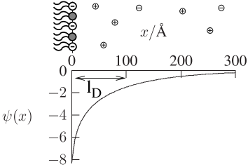
Figure 1: Schematic representation of a binary lipid layer, consisting of negatively charged and neutral lipids. Some co- and counterions are depicted. The graph shows the (reduced) electrostatic potential $\psi(x)$ of a single charged lipid layer with composition $\phi=0.5$ and Debye length $l_{D}=100\>\mbox{\AA}$. Note that into the calculation of $\psi(x)$ also enter $l_{B}=7\>\mbox{\AA}$, and $a=70\>\mbox{\AA}^{2}$. The surface potential for this case is $\Psi=-8.28$; see Eq. 3.

The subject of Poisson-Boltzmann theory is the characterization of the small, mobile, ions in the aqueous solution. These ions reflect the presence of salt with bulk concentration $n_{0}$. In thermal equilibrium, a diffuse ionic layer, consisting of co- and counterions, is built that partially screens the fixed membrane charges. The electrostatic potential $\Phi$ can be calculated if the membrane surface charge density, $\sigma$, the dielectric constant of water, $\epsilon_{W}$, and the salt concentration in the bulk, $n_{0}$, are known. Note that for the flat, large, homogeneous lipid layer in Fig. 1, the electrostatic potential $\Phi=\Phi(x)$ depends only on the $x$-direction.

In Poisson-Boltzmann theory it is convenient to work, instead of $\Phi$, $\epsilon_{W}$, and $n_{0}$, with related quantities, namely with the reduced (dimensionless) electrostatic potential $\psi=e\Phi/k_{B}T$ (where $k_{B}$ is Boltzmann’s constant, and $T$ the absolute temperature), with the Bjerrum length $l_{B}=e^{2}/(4\pi\epsilon_{0}\epsilon_{W}k_{B}T)$, and with the Debye screening length $l_{D}=1/\kappa$, defined through $\kappa^{2}=2e^{2}n_{0}/(\epsilon_{0}\epsilon_{W}k_{B}T)$ (where in the latter two definitions $\epsilon_{0}$ is the permittivity of free space). In terms of these quantities, Poisson-Boltzmann theory leads to the Poisson-Boltzmann equation $\psi^{\prime\prime}(x)=\kappa^{2}\sinh\psi(x)$ that the reduced potential $\psi(x)$ has to fulfill subject to the two boundary conditions $\psi(x\to\infty)=0$ and $\psi^{\prime}(0)=2\kappa p$ where we have used the short notation $p=p_{0}\phi$ with the constant $p_{0}=2\pi l_{B}l_{D}/a$. (Note that a prime denotes the derivative; i. e., $\psi^{\prime}(x)=d\psi(x)/dx$ etc.) Integrating the Poisson-Boltzmann equation once leads with $\psi(x\to\infty)=0$ to

$$\psi^{\prime}(x)=-2\kappa\>\sinh\left(\frac{\psi(x)}{2}\right)$$ (1)

After a second integration we obtain the final solution of the Poisson-Boltzmann equation for a single monolayer

$$\psi(x)=-2\ln\left\{1+\frac{2}{e^{\kappa x}\coth\left[\mbox{arsinh}(p)/2\right]-1}\right\}$$ (2)

which is plotted for one characteristic case in Fig. 1. We note that from Eq. 2 one may obtain the surface potential $\Psi=\psi(x=0)$. The result is

$$\Psi=-2\>\mbox{arsinh}(p_{0}\phi)$$ (3)

For later use we also note that in terms of the surface potential $\Psi$ the potential $\psi(x)$ is given by

$$\psi(x)=-2\ln\left(\frac{e^{\kappa x}-\tanh(\Psi/4)}{e^{\kappa x}+\tanh(\Psi/4)}\right)$$ (4)

Poisson-Boltzmann theory also predicts that the relation between the electrostatic potential and surface charge density can be used to calculate the free energy per lipid through a charging process [Evans and Wennerström, 1994]

$$f_{ml}=a\>\int\limits_{0}^{\sigma}\bar{\Phi}(\tilde{\sigma})\>d\tilde{\sigma}=-k_{B}T\>\int\limits_{0}^{\phi}\Psi(\tilde{\phi})\>d\tilde{\phi}$$ (5)

where $\bar{\Phi}=\Phi(x=0)$ is the electrostatic surface potential. The integration can be carried out because the relation $\Psi(\phi)$ is given in Eq. 3; the result is

$$f_{ml}(\phi)=2\phi\left[\frac{1-q}{p}+\ln(p+q)\right]$$ (6)

with $q=\sqrt{p^{2}+1}$ (recall $p=\phi p_{0}$). Note that here and in the following we shall express all energies in units of $k_{B}T$. Eq. 6 requires $\phi\geq 0$. Yet, the convention $f_{ml}(-\phi)=f_{ml}(\phi)$ ensures applicability of Eq. 6 also for positively charged surfaces where $\phi<0$. Note finally that Eq. 5 implies $f_{ml}^{\prime}(\phi)=-\Psi(\phi)$.

Charged lipid bilayer

A lipid bilayer consists of two apposed lipid monolayers that form a thin film of low dielectric constant. The electrostatic properties on one side of the bilayer may, in principle, depend on those of the other side. This coupling is the subject of the present paragraph.

In the following, we shall refer to the two apposed monolayers of a lipid bilayer as external and internal) and denote their compositions by $\phi_{E}$ and $\phi_{I}$, respectively. Fig. 2 illustrates a number of additional structural properties: The lipid bilayer has hydrophobic thickness $d$ with the charged headgroups of its two monolayers being located at $x=0$ and $x=-d$, and the dielectric constant in the inner hydrophobic region ($-d\leq x\leq 0$) is $\epsilon_{L}$.

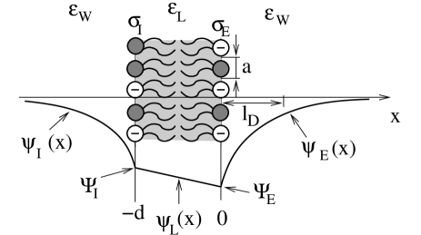
Figure 2: Schematic illustration the lipid bilayer, located within the region $-d<x\leq 0$. The reduced (dimensionless) electrostatic potentials are $\psi_{I}(x)$ and $\psi_{E}(x)$ in the aqueous regions, and $\psi_{L}(x)$ between the charged monolayers, each of surface charge density, $\sigma_{I}=-e\phi_{I}/a$ and $\sigma_{E}=-e\phi_{E}/a$. The reduced surface potentials are denoted by $\Psi_{I}$ and $\Psi_{E}$.

There are three different regions in which we denote the reduced electrostatic potential, $\psi(x)$, by $\psi_{I}(x)$ (for $-\infty<x\leq-d$), by $\psi_{L}(x)$ (for $-d<x\leq 0$), and by $\psi_{E}(x)$ (for $0<x\leq\infty$). The reduced potential then fulfills the Poisson-Boltzmann equation in the aqueous regions adjacent to each monolayer and the Laplace equation inside the membrane

$$\psi_{I}^{\prime\prime}(x) = \kappa^{2}\sinh\psi_{I}\hskip 28.45274ptx\leq-d$$

$$\psi_{L}^{\prime\prime}(x) = 0\hskip 45.52458pt-d<x<0$$ (7)

$$\psi_{E}^{\prime\prime}(x) = \kappa^{2}\sinh\psi_{E}\hskip 28.45274pt0\leq x$$

It is convenient to define a coupling parameter [Winterhalter and Helfrich, 1992] through

$$H=\frac{\epsilon_{L}l_{D}}{\epsilon_{W}d}$$ (8)

With that, the boundary conditions at the two interfacial regions read

$$\psi_{E}^{\prime}(0)-Hd\kappa\psi_{L}^{\prime}(0) = 2\kappa p_{0}\phi_{E}$$

$$-\psi_{I}^{\prime}(-d)+Hd\kappa\psi_{L}^{\prime}(-d) = 2\kappa p_{0}\phi_{I}$$ (9)

Note that, as we expect, for $H=0$ the two conditions reduce to the corresponding ones for two single, electrostatically decoupled, monolayers. The potential between the two charged monolayers fulfills a one-dimensional Laplace equation and is thus given by the linear function,

$$\psi_{L}(x)=\Psi_{I}+\left(1+\frac{x}{d}\right)(\Psi_{E}-\Psi_{I})$$ (10)

where $\Psi_{I}=\psi_{I}(-d)=\psi_{L}(-d)$ and $\Psi_{E}=\psi_{L}(0)=\psi_{E}(0)$ are the surface potentials at the internal and external monolayer, respectively. We thus have $\psi_{L}^{\prime}=\triangle\Psi/d$ where

$$\triangle\Psi=\Psi_{E}-\Psi_{I}$$ (11)

is the difference between the reduced electrostatic potentials across the bilayer. From the first integration of the Poisson-Boltzmann equation (see Eq. 1) and the boundary conditions (see Eqs. Electrostatics of a bare membrane) we find the surface potentials

$$\Psi_{E}=-2\mbox{arsinh}(p_{0}\bar{\phi}_{E})\hskip 28.45274pt\Psi_{I}=-2\mbox{arsinh}(p_{0}\bar{\phi}_{I})$$ (12)

where we have introduced the effective compositions

$$\bar{\phi}_{E}=\phi_{E}+\frac{H\triangle\Psi}{2p_{0}}\hskip 28.45274pt\bar{\phi}_{I}=\phi_{I}-\frac{H\triangle\Psi}{2p_{0}}$$ (13)

We note that the surface potentials, $\Psi_{E}=\Psi_{E}(\phi_{E},\phi_{I})$ and $\Psi_{E}=\Psi_{E}(\phi_{E},\phi_{I})$, depend on both monolayer compositions, $\phi_{E}$ and $\phi_{I}$, because of the electrostatic coupling between the charged monolayers. Combination of Eq. 12 and Eq. 13 leads to $\triangle\Psi=f_{ml}^{\prime}(\bar{\phi}_{I})-f_{ml}^{\prime}(\bar{\phi}_{E})$ or, equivalently,

$$\frac{\triangle\Psi}{2}=\mbox{arsinh}\left(p_{0}\phi_{I}-\frac{H}{2}\triangle\Psi\right)-\mbox{arsinh}\left(p_{0}\phi_{E}+\frac{H}{2}\triangle\Psi\right)$$ (14)

which represents a transcendental equation for the potential difference $\triangle\Psi$ across the membrane [Baciu and May, 2004]. Of course, for a symmetric bilayer, where $\phi_{E}=\phi_{I}$, the solution of Eq. 14 is $\triangle\Psi=0$.

The electrostatic free energy, $f_{bl}$ (measured per lipid pair) is given by a charging process analogous to Eq. 5

$$f_{bl}=-\int\limits_{0}^{\phi_{I}}\Psi_{I}(\tilde{\phi}_{I},0)d\tilde{\phi}_{I}-\int\limits_{0}^{\phi_{E}}\Psi_{E}(\phi_{I},\tilde{\phi}_{E})d\tilde{\phi}_{E}$$ (15)

where here we first charge the internal monolayer, and then the external one (any other path of charging would lead to the same result). We obtain

$$\framebox{$\displaystyle f_{bl}=f_{ml}(\bar{\phi}_{E})+f_{ml}(\bar{\phi}_{I})+\frac{H}{4p_{0}}\triangle\Psi^{2}$}$$ (16)

The first two terms represent the charging energies for two single monolayers of effective compositions $\bar{\phi}_{E}$ and $\bar{\phi}_{I}$. The last term, $H\triangle\Psi^{2}/4p_{0}=\epsilon_{L}a\triangle\bar{\Phi}^{2}/2d$ is the contribution of the capacitor between the charged monolayer interfaces where $\triangle\bar{\Phi}$ is the potential difference between the external and internal monolayer.

For $H=0$ there is no electrostatic coupling between the charged monolayers. In this case, $f_{bl}=f_{ml}(\phi_{E})+f_{ml}(\phi_{I})$ is given by the sum of the individual free energies of two isolated monolayers.

Macroion-bilayer interaction

After heaving dealt with a bare lipid bilayer, we are now in the position to add a positively charged macroion to the external side of the bilayer. To be specific, we place the charges of the macroion at position $h$ along the $x$-axis as shown in Fig. 3 below. It is convenient to express the charge density, $\sigma_{P}=\phi_{P}e/a$, of the macroion in terms of the compositional variable $\phi_{P}$ (with $0\leq\phi_{P}\leq 1$). For $\phi_{P}=\phi_{E}$ the charge densities on the macroion and on the external monolayer match each other; that is, they would be opposite in sign and equal in magnitude.

As for the isolated bilayer, the potentials, $\psi_{I}(x)$, $\psi_{L}(x)$, and $\psi_{E}(x)$, are determined by Eqs. Electrostatics of a bare membrane. The only difference is that the last one of Eqs. Electrostatics of a bare membrane applies only within the region, $0\leq x\leq h$, between the external monolayer and the macroion. The boundary condition at the macroion is $\psi_{E}^{\prime}(h)=2\kappa p_{0}\phi_{P}$. The other two boundary conditions (see Eq. Electrostatics of a bare membrane) remain unchanged. The surface potentials $\Psi_{I}=\psi_{I}(-d)=\psi_{L}(-d)$, $\Psi_{E}=\psi_{L}(0)=\psi_{E}(0)$, and $\Psi_{P}=\psi_{E}(h)$ depend on the three compositions, $\phi_{I}$, $\phi_{E}$, and $\phi_{P}$. We thus write $\Psi_{I}=\Psi_{I}(\phi_{I},\phi_{E},\phi_{P})$, $\Psi_{E}=\Psi_{E}(\phi_{I},\phi_{E},\phi_{P})$, and $\Psi_{P}=\Psi_{P}(\phi_{I},\phi_{E},\phi_{P})$. Fig. 3 schematically illustrates the macroion-bilayer system.

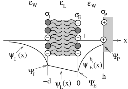
Figure 3: Schematic illustration the lipid bilayer, interacting with a macroion. The difference to Fig. 2 is the presence of the positively charged macroion of surface charge density $\sigma_{P}=e\phi_{P}/a$ at position $x=h$. The surface potential at the macroion is denoted by $\Psi_{P}$. (Depicted is the case of a weakly charged macroion.)

The free energy of the macroion-membrane system, measured per lipid in one monolayer, is again given by the familiar charging process analogous to Eq. 15

$$f = -\int\limits_{0}^{\phi_{I}}\Psi_{I}(\tilde{\phi}_{I},0,0)d\tilde{\phi}_{I}-\int\limits_{0}^{\phi_{E}}\Psi_{E}(\phi_{I},\tilde{\phi}_{E},0)d\tilde{\phi}_{E}$$ (17)

$$+ \int\limits_{0}^{\phi_{P}}\Psi_{P}(\phi_{I},\phi_{E},\tilde{\phi}_{P})d\tilde{\phi}_{P}$$

It corresponds to charging first the internal monolayer (first term in Eq. 17), then the external monolayer (second term in Eq. 17), and finally the macroion (last term in Eq. 17). We repeat that the final result for $f$ does of course not depend on the order in which the surfaces are charged.

In the following, the distance $h$ between the macroion and the bilayer is chosen such that the free energy $f$ is minimal. In this case, the potential $\psi_{E}(x)$ has the same functional form as for an isolated charged monolayer [Parsegian and Gingell, 1972]: for small $\phi_{P}$ the potential is that of the isolated lipid bilayer, and for large $\phi_{P}$ the potential is determined solely by the macroion charges. The small and large $\phi_{P}$ cases are separated by another, intermediate, regime where the macroion contacts the bilayer (implying $h=0$). In the following, we shall consider the three possible scenarios separately.

Weakly charged macroion

If $\phi_{P}$ is sufficiently low the potential $\psi(x)$ is equivalent to that of an isolated bilayer within the region $-\infty\leq x\leq h$. The surface potentials at the membrane are thus, again, given by Eq. 12, and the value of the potential at the macroion,

$$\Psi_{P}=-2\mbox{arsinh}(p_{0}\phi_{P})$$ (18)

is negative. Recalling the functional form of Eq. 4 and $\psi_{E}(h)=\Psi_{P}$, it follows that

$$e^{\kappa h}=\frac{\tanh\left(\Psi_{E}/4\right)}{\tanh\left(\Psi_{P}/4\right)}=\left(\frac{\phi_{P}}{\bar{\phi}_{E}}\right)\>\left(\frac{\sqrt{1+(p_{0}\bar{\phi}_{E})^{2}}-1}{\sqrt{1+(p_{0}\phi_{P})^{2}}-1}\right)$$ (19)

which allows us to calculate the equilibrium distance, $h$, between the macroion and the external monolayer. With growing $\phi_{P}$ the distance $h$ decreases until close contact is established for a particular $\phi_{P}$ which fulfills the relation $\phi_{P}=\bar{\phi}_{E}$. The condition

$$\phi_{P}<\phi_{E}+\frac{H}{2p_{0}}\triangle\Psi$$ (20)

thus defines the weakly charged macroion regime. Recall that the potential difference, $\triangle\Psi$, fulfills Eq. 14. The presence of the oppositely charged macroion reduces the free energy of the isolated bilayer by the charging free energy of the isolated macroion

$$\framebox{$\displaystyle f=f_{ml}(\bar{\phi}_{E})+f_{ml}(\bar{\phi}_{I})+\frac{H}{4p_{0}}\triangle\Psi^{2}-f_{ml}(\phi_{P})$}$$ (21)

Highly charged macroion

For sufficiently high $\phi_{P}$, the potential between the macroion and the external monolayer ($0\leq x\leq h$) is equal to that of the isolated macroion, implying

$$\psi_{E}(x)=-2\ln\left(\frac{e^{-\kappa(x-h)}-\tanh(\Psi_{P}/4)}{e^{-\kappa(x-h)}+\tanh(\Psi_{P}/4)}\right)$$ (22)

Hence, both the surface potentials at the macroion and at the external monolayer are positive,

$$\Psi_{E}=2\mbox{arsinh}(p_{0}\bar{\phi}_{E})\hskip 28.45274pt\Psi_{P}=2\>\mbox{arsinh}(p_{0}\phi_{P})$$ (23)

whereas the surface potential of the internal monolayer

$$\Psi_{I}=-2\mbox{arsinh}(p_{0}\bar{\phi}_{I})$$ (24)

can be either negative ($\bar{\phi}_{I}>0$) or positive ($\bar{\phi}_{I}<0$), depending on the sign of $\bar{\phi}_{I}$. Inserting the definitions for $\bar{\phi}_{I}$ and $\bar{\phi}_{E}$ (see Eqs. 13) we find a transcendental equation for the potential difference $\triangle\Psi$ across the bilayer

$$\frac{\triangle\Psi}{2}=\mbox{arsinh}\left(p_{0}\phi_{I}-\frac{H}{2}\triangle\Psi\right)+\mbox{arsinh}\left(p_{0}\phi_{E}+\frac{H}{2}\triangle\Psi\right)$$ (25)

Because of $\Psi_{E}=\psi_{E}(0)$ according to Eq. 22, and with Eq. 23, we can determine the equilibrium distance $h$ through

$$e^{\kappa h}=\frac{\tanh\left(\Psi_{P}/4\right)}{\tanh\left(\Psi_{E}/4\right)}=\left(\frac{\bar{\phi}_{E}}{\phi_{P}}\right)\>\left(\frac{\sqrt{1+(p_{0}\phi_{P})^{2}}-1}{\sqrt{1+(p_{0}\bar{\phi}_{E})^{2}}-1}\right)$$ (26)

With decreasing $\phi_{P}$ the distance $h$ decreases too until close contact is established for a particular $\phi_{P}$ which fulfills the relation $\phi_{P}=\bar{\phi}_{E}$. Hence, the highly charged macroion regime is defined by the condition

$$\phi_{P}>\phi_{E}+\frac{H}{2p_{0}}\triangle\Psi$$ (27)

where, the potential difference, $\triangle\Psi$, results from the solution of Eq. 25. Note that the surface potential at the internal monolayer, $\Psi_{I}$, is positive if $H\triangle\Psi>2p_{0}\phi_{I}$, and combination with Eq. 27 reveals that $\phi_{P}>\phi_{E}+\phi_{I}$ is a necessary condition to reverse the sign of both surface potentials, $\Psi_{I}$ and $\Psi_{E}$.

The presence of the macroion leads to the free energy

$$\framebox{$\displaystyle f=-f_{ml}(\bar{\phi}_{E})+f_{ml}(\bar{\phi}_{I})+\frac{H}{4p_{0}}\triangle\Psi^{2}+f_{ml}(\phi_{P})$}$$ (28)

Intermediate case: Close contact

In between the weakly and highly charged macroion regimes (defined by Eq. 20 and Eq. 27) the macroion and the external monolayer are at close contact. Here, the surface potentials at the lipid bilayer are determined by the equations

$$\Psi_{I} = -2\>\mbox{arsinh}[p_{0}(\phi_{I}+\phi_{E}-\phi_{P})]$$ (29)

$$\Psi_{E} = -2\>\mbox{arsinh}[p_{0}(\phi_{I}+\phi_{E}-\phi_{P})]-\frac{2p_{0}}{H}(\phi_{E}-\phi_{I})$$

Note that because of $h=0$ it is $\Psi_{E}=\Psi_{P}$. The free energy can be calculated by the usual charging process

$$f=-\int\limits_{0}^{\phi_{I}}\Psi_{I}(\tilde{\phi}_{I},\phi_{E}-\phi_{P}=0)\>d\tilde{\phi}_{I}-\int\limits_{0}^{\phi_{E}-\phi_{P}}\Psi_{E}(\phi_{I},\tilde{\phi})\>d\tilde{\phi}$$ (30)

which corresponds to first charging the internal monolayer and then the together the external layer and the macroion. We obtain the result

$$\framebox{$\displaystyle f=f_{ml}(\phi_{I}+\phi_{E}-\phi_{P})+\frac{p_{0}}{H}{(\phi_{E}-\phi_{P})}^{2}$}$$ (31)

which is the sum of the electrostatic free energy of a single isolated monolayer of composition $|\phi_{I}+\phi_{E}-\phi_{P}|$ and the capacitor energy $H\triangle\Psi^{2}/4p_{0}$. Note the particular case $\phi_{P}=\phi_{E}+\phi_{I}$ for which $f=p_{0}\phi_{I}^{2}/H$.

Two limiting cases

The free energies $f$ in Eqs. 21, 28 and 31 cover all possible interaction regimes of a macroion with an oppositely charged lipid bilayer. The actual calculation of $f$, however, requires to solve an additional transcendental equation for $\triangle\Psi$. There are two limiting cases for which $f$ can be expressed directly in terms of the membrane and macroion charge densities. One is the Debye-Hückel limit which is based on linearizing the Poisson-Boltzmann equation. The other one corresponds to a very thin (transparent) lipid bilayer for which the limit $d\to 0$ may be considered. These two cases are discussed in the following.

Debye-Hückel limit

For sufficiently small charge densities the Poisson-Boltzmann equation can be linearized. Formally, the Debye-Hückel case may be viewed as the limit corresponding to $l_{D}\to 0$ (or, equivalently, $p_{0}\to 0)$. In this case, all three regimes of the interacting macroion-bilayer system can be calculated explicitly.

In the weakly charged macroion regime linearization of Eq. 14 gives rise to

$$\triangle\Psi=-2p_{0}\>\frac{\phi_{E}-\phi_{I}}{1+2H}$$ (32)

We can use this result to calculate the condition for the system to be in the weakly charged macroion regime (see Eq. 20)

$$\phi_{P}<\phi_{E}-\frac{H}{1+2H}\>(\phi_{E}-\phi_{I})$$ (33)

as well as the relation for the distance, $h$, between the macroion and the external monolayer (see Eq. 19)

$$e^{\kappa h}=\frac{\phi_{E}+H(\phi_{E}+\phi_{I})}{\phi_{P}(1+2H)}$$ (34)

and the free energy (see Eq. 21)

$$\frac{f}{p_{0}}=\phi_{I}^{2}+\phi_{E}^{2}-\phi_{P}^{2}-\frac{H}{1+2H}(\phi_{E}-\phi_{I})^{2}$$ (35)

Similarly in the highly charged macroion regime, linearization of Eq. 25 results in

$$\triangle\Psi=2p_{0}(\phi_{E}+\phi_{I})$$ (36)

This result is used to calculate the condition for the system to reside in the highly charged macroion regime (see Eq. 27)

$$\phi_{P}>\phi_{E}+H(\phi_{E}+\phi_{I})$$ (37)

as well as the relation for the distance, $h$, between the macroion and the external monolayer (see Eq. 26)

$$e^{\kappa h}=\frac{\phi_{P}}{\phi_{E}+H(\phi_{E}+\phi_{I})}$$ (38)

and the free energy (see Eq. 28)

$$\frac{f}{p_{0}}=\phi_{I}^{2}-\phi_{E}^{2}+\phi_{P}^{2}-H(\phi_{E}+\phi_{I})^{2}$$ (39)

Finally, for the intermediate case of close contact, Eq. 31 already provides an explicit expression which in the Debye-Hückel limit reads

$$\frac{f}{p_{0}}=(\phi_{I}+\phi_{E}-\phi_{P})^{2}+\frac{1}{H}\>(\phi_{E}-\phi_{P})^{2}$$ (40)

Of course, at the transition from one regime into the other the free energy is continuous (but not necessarily smooth). That is, for $\phi_{P}=\phi_{E}-(\phi_{E}-\phi_{I})H/(1+2H)$, the free energy $f$ in Eq. 35 is equal to that in Eq. 40. Similarly, for $\phi_{P}=\phi_{E}+H(\phi_{E}+\phi_{I})$, the free energy $f$ in Eq. 39 is equal to that in Eq. 40.

Transparent bilayer

For very thin membranes ($d\to 0$) or in the limit of large Debye length ($l_{D}\to\infty$) it is $H\to\infty$, and the membrane appears transparent to the electric field.

Consider first the low macroion charge limit. For $H\to\infty$ we obtain from Eq. 14 the potential difference

$$\triangle\Psi=-\frac{p_{0}}{H}\>(\phi_{E}-\phi_{I})\to 0$$ (41)

The effective compositions, defined in Eq. 13, are then simply

$$\bar{\phi}_{E}=\bar{\phi}_{I}=\frac{1}{2}\>(\phi_{E}+\phi_{I})$$ (42)

We also see that the condition for residing in the weakly charged macroion regime becomes $\phi_{P}<\bar{\phi}$ where we have defined the average composition of the lipid bilayer $\bar{\phi}=(\phi_{I}+\phi_{E})/2$. The distance between the macroion and the external monolayer is again given by Eq. 19 with $\bar{\phi}_{E}=\bar{\phi}$. Finally, the free energy (see Eq. 21) becomes

$$f=2f_{ml}(\bar{\phi})-f_{ml}(\phi_{P})$$ (43)

For $\phi_{P}>\bar{\phi}$ there is close contact between the external monolayer and the macroion. A third, high macroion charge regime, does not exist for a transparent membrane. In the close contact regime, Eq. 31 predicts $f=f_{ml}(\phi_{I}+\phi_{E}-\phi_{P})$.

Electrostatic coupling between the DNA monolayers in lamellar lipoplexes

In this section we shall apply our results for the electrostatic coupling to a specific system, the lamellar lipoplex. As mentioned in the Introduction, there is experimental evidence for the orientational alignment of the DNA arrays across the cationic bilayers [Battersby et al., 1998]. Such an alignment implies some kind of energetic coupling. Our results from the previous sections enable us to calculate the electrostatic contribution to this coupling. Fig. 4 depicts the structure of the lamellar lipoplex with its one-dimensional arrays of DNA monolayers being intercalated between a stack of cationic bilayers.

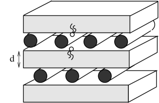
Figure 4: Schematic illustration of the lamellar lipoplex structure. The (double stranded) DNA molecules, depicted as long rods, form one-dimensional arrays between each pair of cationic bilayers. Arrays in consecutive membrane galleries are orientationally aligned and shifted ”out of phase”. Some lipids are schematically shown; $d$ denotes the membrane thickness.

Our objective is to use the formalism developed in the previous sections to (roughly) estimate the interaction strength of the DNA molecules through a charged lipid bilayer. To do so, it is convenient to consider only a single, perfectly planar, cationic lipid bilayer with two oppositely charged DNA arrays attached to each of its apposed monolayers. Assuming all DNA strands to be parallel we shift one array with respect to the other one. The corresponding free energy is expected to adopt its minimum and maximum for the two DNA arrays being ”out of phase” and ”in phase”, respectively (see states A and B in Fig. 5).

At this point it should be noted that the recent theoretical prediction of a so-called sliding columnar phase is based not only on an energetic penalty of laterally shifting the two DNA arrays (as shown in Fig. 5) but also on a second energy contribution associated with angular changes of the DNA arrays with respect to each other [O’Hern and Lubensky, 1998, Golubovic and Golubovic, 1998]. Clearly, our present simplified model allows to estimate the former but not the latter contribution.

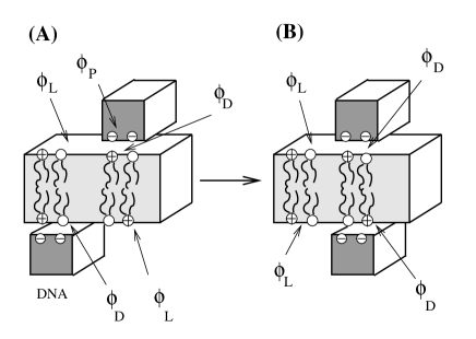
Figure 5: Our structural model to calculate the degree of electrostatic coupling of two DNA rods (depicted with rectangular cross-section) across a cationic bilayer: in state (A) the DNA rods are ”out of phase” so that potential gradients along the membrane normal direction can form. In state (B) the DNA rods are ”in phase”, implying transmembrane symmetry and thus vanishing gradients. The difference in free energy of states (A) and (B) is a measure for the degree of electrostatic coupling. Note that, in general, the mixed cationic membrane may optimize its composition (mole fraction of charged lipids); $\phi_{D}$ and $\phi_{L}$ denote the compositions at the DNA adsorption region and at the bare membrane, respectively.

We calculate the corresponding free energy difference, $\triangle F$, between states A and B per persistence length, $\xi=500\>\mbox{\AA}$, of double stranded DNA. Let us denote by $N$ the number of lipids that interact electrostatically with the DNA. There is some arbitrariness in choosing $N$ because the planar macroion geometry (see Fig. 5) is not a very realistic model for a DNA molecule. Still a reasonable estimate is $N=2\xi R_{D}/a\approx 150$ where $R_{D}=10\>\mbox{\AA}$ is the radius of the DNA rod (typically, $a\approx 70\>\mbox{\AA}^{2}$ is the cross-sectional area per lipid). The additional factor of two in $N=2\xi R_{D}/a$ results from the two monolayers that interact with a single DNA molecule.

The main difference of states A and B in Fig. 5 is the symmetry of state B with respect to the bilayer’s midplane. That is, for state B the potential difference across the bilayer $\triangle\Psi$ vanishes (corresponding to $H=0$) and we can write for the difference in free energy between state A and B

$$\triangle F=F_{A}-F_{B}=N[f(\phi,H)-f(\phi,H=0)]$$ (44)

where $f$ is the free energy per lipid in one monolayer, and is given by Eq. 21 for low macroion charge, by Eq. 31 for close contact, and by Eq. 28 for high macroion charge.

To specify the compositional variable $\phi$ in Eq. 44 we note the ability of the lipid bilayer to adjust its local lipid composition. That is, close to the DNA adsorption site the local lipid composition, which we shall denote by $\phi_{D}$, may differ from that at the DNA-free bilayer region (denoted by $\phi_{L}$ in the following). The ability for local demixing can (approximatively) be included in our calculation of $\triangle F$. In order to derive an explicit relation we shall assume small electrostatic coupling $H\ll 1$ for which we can expand $\triangle F$ up to first order in $H$. The result is

$$\triangle F=-\frac{NH}{4p_{0}}\>[\triangle\Psi(\phi_{D},\phi_{L})]^{2}=-\frac{NH}{4p_{0}}\>\left[f_{ml}^{\prime}(\phi_{D})\mp f_{ml}^{\prime}(\phi_{L})\right]^{2}$$ (45)

where the minus sign refers to the low and the plus sign to the high macroion charge regime (in the small $H$ limit the small macroion charge regime is $\phi_{P}<\phi_{D}$ and the high macroion charge regime is $\phi_{P}>\phi_{D}$; the close contact regime reduces to $\phi_{P}=\phi_{D}$).

Let us analyze the consequences of Eq. 45. For frozen lipid composition, where $\phi_{D}=\phi_{L}=\phi$, we find $\triangle F=0$ in the low macroion charge regime. This is expected because for low $\phi_{P}$ the macroions do not affect the membrane potentials. Yet, the membrane is symmetric, implying $\triangle\Psi=0$, and the electrostatic coupling across the bilayer is irrelevant.

Consider now the high macroion charge regime for frozen lipid composition ($\phi_{D}=\phi_{L}=\phi$). Here Eq. 45 becomes

$$\triangle F=-4N\frac{H}{p_{0}}\>\mbox{arsinh}^{2}(p_{0}\phi)$$ (46)

In Fig. 6 we plot $\triangle F$ according to Eq. 46 (with $H=\epsilon_{L}l_{D}/\epsilon_{W}d$ and $p_{0}=2\pi l_{D}l_{B}/a$) for $l_{B}=7\>\mbox{\AA}$, $a=70\>\mbox{\AA}^{2}$, $N=150$, $\epsilon_{W}/\epsilon_{L}=40$, and $d=30\>\mbox{\AA}$ as a function of the Debye length $l_{D}$. Curve (a) is derived for $\phi=0.5$, curve (b) for $\phi=0.25$. In both cases $\triangle F$ can become considerably larger than $k_{B}T$ under low salt conditions.

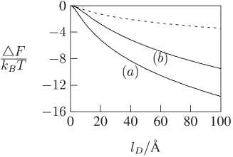
Figure 6: $\triangle F$ according to Eq. 46 for $l_{B}=7\>\mbox{\AA}$, $a=70\>\mbox{\AA}^{2}$, $N=80$, $\epsilon_{W}/\epsilon_{L}=40$, and $d=30\>\mbox{\AA}$ as a function of the Debye length $l_{D}$. The two curves correspond to $\phi=0.5$ (a) and $\phi=0.25$, (b). The broken line shows $\triangle F$ according to Eq. 47 for $\phi_{P}=0.5$.

Let us also estimate the influence of local lipid demixing. To this end we consider a weakly charged membrane. The presence of the DNA’s induces accumulation of charged lipids near the DNA. From an electrostatic point of view, local charge matching ($\phi_{D}\approx\phi_{P}$) would be the optimal situation. The matching $\phi_{D}=\phi_{P}$ would be opposed by the demixing free energy of the lipids but we may still consider the limiting situation that all charged lipids are driven towards the DNA adsorption site, implying $\phi_{D}=\phi_{P}$ and $\phi_{L}=0$. Eq. 45 then reads

$$\triangle F=-N\frac{H}{p_{0}}\>\mbox{arsinh}^{2}(p_{0}\phi_{P})$$ (47)

Comparison of Eq. 46 with Eq. 47 shows that the lateral mobility of the lipids tends to reduce the electrostatic coupling of the DNA arrays through the cationic bilayer. Sufficiently strong electrostatic coupling is generally found only if the Debye length is considerably larger than that under physiological conditions where $l_{D}\gg 10\>\mbox{\AA}$.

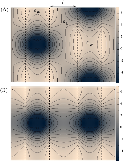
Figure 7: Simulation results for the potential $\Psi({\bf r})$ in a lamellar lipoplex. The two diagrams correspond to the ”out of phase” (A) and ”in phase” (B) cases (see also Fig. 5). Contour lines are drawn at integer values of $\Psi$. The simulation is carried out for a 112 Åx 160 Åsystem. The membrane width is $d=30\mbox{\AA}$, the DNA radius is $R_{D}=10\mbox{\AA}$, and the distance between the DNA and the membrane is $3\mbox{\AA}$. We use $l_{D}=100\mbox{\AA}$, $l_{B}=7\mbox{\AA}$ and $\epsilon_{L}/\epsilon_{W}=1/40$. The membrane is homogeneously charged with composition $\phi=0.25$ of monovalent cationic lipids. The charge density on the DNA is twice as large as that on the membrane, amounting to a linear charge density of $-e/1.7\mbox{\AA}$ along each DNA rod. The location of the membrane charges is indicated by the vertical dashed lines.

Solving the Poisson-Boltzmann equation using the lattice Boltzmann method

For our numerical calculations we developed a lattice Boltzmann method who’s stationary state solves the Poisson-Boltzmann equation in the unit cell of the lamellar lipoplex geometry. The lattice Boltzmann method simulates densities $f_{i}$ on a lattice. Each of these densities is associated with a velocity ${\bf v}_{i}$ and they evolve with (scaled) time $t$ through the lattice Boltzmann equation

$$f_{i}({\bf r}+{\bf v}_{i},t+1)=f_{i}({\bf r},t)+\frac{1}{\tau({\bf r})}[f_{i}^{0}({\bf r},t)-f_{i}({\bf r},t)].$$ (48)

We identify the potential $\Psi({\bf r},t)=\sum_{i}f_{i}({\bf r},t)$ and choose the distribution $f_{i}^{0}$ such that it has the moments

$$\sum_{i}f_{i}^{0} = \tau({\bf r})\frac{\theta({\bf r})\kappa^{2}\sinh(\Psi)+2\pi l_{B}\rho_{f}({\bf r})}{6}-\Psi({\bf r},t),$$

$$\sum_{i}f_{i}^{0}{\bf v}_{i} = 0,$$ (49)

$$\sum_{i}f_{i}^{0}{\bf v}_{i}{\bf v}_{i} = \frac{\Psi(x,t)}{3}\mathbf{1}.$$

We further choose $\tau({\bf r})=[\epsilon({\bf r})/\epsilon_{W}+1]/2$. Summing equation (48) we obtain the macroscopic equation

$$\frac{\partial\Psi({\bf r},t)}{\partial t}+\nabla\left(\frac{\epsilon({\bf r})}{\epsilon_{W}}\nabla\Psi({\bf r},t)\right)=\theta({\bf r})\kappa^{2}\sinh\left(\Psi({\bf r},t)\right)+\rho_{f}({\bf r})$$ (50)

so that the stationary solutions of this simulation solves the Poisson-Boltzmann equation for fixed input charge density $\rho_{f}({\bf r})$ and a given field of dielectric constants $\epsilon({\bf r})$. The step function $\theta({\bf r})$ determines the accessibility of the space to salt ions. Further details on the method will be given elsewhere.

We set up a simulation with two lipid bilayers and two DNA molecules imposing periodic boundary conditions. In our simulations one lattice spacing corresponds to $1\>\mbox{\AA}$. We exclude salt ions from the membrane regions and from the interior of the DNA (this is achieved by the step function $\theta({\bf r})$ in Eq. 50) and calculate the free energy $\triangle F(x_{rel})$ as a function of the scaled lateral displacement $x_{rel}$ of the DNA arrays in consecutive galleries of the lipoplex. A snapshot of the potential $\Psi({\bf r})$ calculated by our simulations is shown in Fig. 7. The resulting free energy per unit length is then multiplied with the persistence length of the DNA, $\xi=500\>\mbox{\AA}$, to give the change in free energy with the displacement $x_{rel}$ in units of $k_{B}T$. This result is shown in Fig. 8 and is in good agreement with the theoretical prediction of Eq. 46. More specifically, Fig. 8 predicts a maximal change of $\triangle F\approx-9k_{B}T$ which happens to coincide with the corresponding value of curve (b) in Fig. 6 for $l_{D}=100\mbox{\AA}$.

Figure 8: Numerical results (derived for the same parameters as those in Fig. 7) for the change of the free energy $\triangle F$ with the relative displacement $x_{rel}$ of the DNA arrays with respect to each other. The free energies corresponding to the systems shown in Fig. 7 are indicated by (A) and (B).

To sum up, the validity of our approximate analytical model for the electrostatic coupling of the two monolayers in a lipid membrane is supported by the numerical solutions of the Poisson-Boltzmann equation (based on the lattice Boltzmann method). Generally, the electrostatic communication across a lipid bilayer is quite weak due to the large drop of the dielectric constant inside the membrane. However, as we have shown for a lamellar lipoplex, it cannot always be neglected.

Conclusions

The electrostatic interaction of a macroion with an oppositely charged lipid bilayer depends on the coupling parameter $H=\epsilon_{L}l_{D}/(\epsilon_{W}d)$. In the (hypothetical) limit $H=0$ the interaction reduces to that between the macroion and a single monolayer. Here, the apposed monolayer – separated from the macroion by a slab of low dielectric constant – can be ignored completely. Differently expressed, for $H=0$ the two monolayers of a lipid bilayer are electrostatically decoupled.

For non-vanishing values of $H$ the behavior of the macroion-membrane complex is influenced by the electrostatic interaction through the hydrocarbon core of the lipid membrane. We have studied this aspect on the basis of Gouy-Chapman theory, solving a one-dimensional Poison-Boltzmann equation. (Thus, all approximations inherent in the Poison-Boltzmann formalism are also present in this work). We find interesting and non-trivial behavior for non-vanishing $H$, characterized by three different regimes: A single weakly charged macroion does not affect the surface potentials on either one of the two membrane leaflets. As the surface charge of the macroion is increased, a regime of close contact will be passed, leading ultimately to a third regime of high macroion charge where the sign of the electrostatic membrane potential, either on one or on both membrane leaflets, is reversed. Within our one-dimensional model, all characteristic quantities such as membrane potentials, macroion-membrane distance, free energies, and boundaries between the different regimes can be calculated analytically.

Typically, the ratio between the dielectric constants inside the membrane ($\epsilon_{L}$) and in the water phase ($\epsilon_{W}$) is very small, $\epsilon_{L}/\epsilon_{W}\approx 1/40$. Thus, only for large ratio between the Debye length ($l_{D}$) and the membrane thickness $d$ is $H$ not small compared to $1$. Yet, even for $H\ll 1$ electrostatic interactions across a lipid membrane can be relevant. To this end, we have estimated the electrostatic interaction between the ordered DNA arrays in different galleries of the lamellar $L_{\alpha}^{C}$ lipoplex structure. For sufficiently large Debye length $l_{D}$ we find a significant electrostatic contribution to the experimentally observed inter-locking of orientationally ordered DNA arrays across different galleries.

Finally, the present work employs the Lattice-Boltzmann method to solve the Poisson-Boltzmann equation for the lamellar $L_{\alpha}^{C}$ lipoplex structure. Our numerical calculations account for the structural details of the $L_{\alpha}^{C}$ lipoplex and compare well with the analytical results derived on the basis of the one-dimensional Poisson-Boltzmann model. We thus believe that the one-dimensional model is a useful tool to estimate interactions between macroions across a lipid bilayer.

Acknowledgments SM would like to thank Anne Hinderliter and, during the early stages of this work, Cristina Baciu for discussions. AJW acknowledges discussions with Eric Foard. This work was supported by NIH Grant 1 R15 GM077184-01.

References

- Andelman, 1995 Andelman, D. 1995. Electrostatic properties of membranes: The Poisson-Boltzmann theory. Section 12, pages 603–642 of: Lipowsky, R., and Sackmann, E. (eds), Structure and Dynamics of Membranes, second edn., vol. 1. Amsterdam: Elsevier.
- Baciu and May, 2004 Baciu, C. L., and May, S. 2004. Stability of charged, mixed lipid bilayers: effect of electrostatic coupling between the monolayers. Journal of Physics-Condensed Matter, 16, S2455–S2460.
- Battersby et al., 1998 Battersby, B. J., Grimm, R., Hübner, S., and Cevc, G. 1998. Evidence for three-dimensional interlayer correlations in cationic lipid-DNA complexes as observed by cryo-electron microscopy. Biophys. Biochim. Acta., 1372, 379–383.
- Chen and Nelson, 2000 Chen, Y., and Nelson, P. 2000. Charge-reversal instability in mixed bilayer vesicles. Phys. Rev. E, 62, 2608–2619.
- Dalal et al., 2006 Dalal, P., Zanotti, K., Wierzbicki, A., Madura, J. D., and Cheung, H. C. 2006. Molecular dynamics simulation studies of the effect of phosphocitrate on crystal-induced membranolysis. Biophys. J., 89, 2251–2257.
- de Lima et al., 2001 de Lima, M. C Pedroso, Simões, S., Pires, P., Faneca, H., and Düzgünes, N. 2001. Cationic lipid-DNA complexes in gene delivery: from biophysics to biological applications. Adv. Drug. Deliv. Rev., 47, 277–294.
- Evans and Wennerström, 1994 Evans, D. F., and Wennerström, H. 1994. The colloidal domain, where physics, chemistry, and biology meet. Second edn. VCH publishers.
- Genet et al., 2000 Genet, S., Costalat, R., and Burger, J. 2000. A few comments on electrostatic interactions in cell physiology. Acta Biotheoretica, 48, 273–287.
- Golubovic and Golubovic, 1998 Golubovic, L., and Golubovic, M. 1998. Fluctuations of quasi-two-dimensional smectics intercalated between membranes in multilamellar phases of DNA cationic lipid complexes. Phys. Rev. Lett., 80, 4341–4344.
- Harries et al., 2003 Harries, D., May, S., and Ben-Shaul, A. 2003. Curvature and charge modulations in lamellar DNA-lipid complexes. J. Phys. Chem. B., 107, 3624–3630.
- Horbach and Frenkel, 2001 Horbach, J., and Frenkel, D. 2001. Lattice-Boltzmann method for the simulation of transport phenomena in charged colloids. Phys. Rev. E, 64, 061507.
- Israelachvili, 1992 Israelachvili, J. N. 1992. Intermolecular and Surface Forces. Second edn. Academic Press.
- Lasic et al., 1997 Lasic, D. D., Strey, H., Stuart, M. C. A., Podgornik, R., and Frederik, P. M. 1997. The structure of DNA-liposome complexes. J. Am. Chem. Soc., 119, 832–833.
- Nelson et al., 1975 Nelson, A. P., Colonomos, P., and McQuarrie, D. A. 1975. Electrostatic coupling across a membrane with titratable surface groups. J. Theor. Biol., 50, 317–325.
- O’Hern and Lubensky, 1998 O’Hern, C. S., and Lubensky, T. C. 1998. Sliding columnar phase of DNA lipid complexes. Phys. Rev. Lett., 80, 4345–4348.
- Parsegian and Gingell, 1972 Parsegian, V. A., and Gingell, D. 1972. On the electrostatic interaction across a salt solution between two bodies bearing unequal charges. Biophys. J., 12, 1192–1204.
- Rädler et al., 1997 Rädler, J. O., Koltover, I., Salditt, T., and Safinya, C. R. 1997. Structure of DNA-cationic liposome complexes: DNA intercalation in multilamellar membranes in distinct interhelical packing regimes. Science, 275, 810–814.
- Schiessel and Aranda-Espinoza, 2001 Schiessel, H., and Aranda-Espinoza, H. 2001. Electrostatically induced undulations of lamellar DNA-lipid complexes. Eur. Phys. J. E, 5, 499–506.
- Taheri-Araghi and Ha, 2005 Taheri-Araghi, S., and Ha, B. Y. 2005. Charge renormalization and inversion of a highly charged lipid bilayer: effects of dielectric discontinuities and charge correlations. Phys. Rev. E, 72, 021508.
- Winterhalter and Helfrich, 1992 Winterhalter, M., and Helfrich, W. 1992. Bending Elas- ticity of Electrically Charged Bilayers:Coupled Monolay- ers, Neutral Surfaces, and Balancing Stresses. J. Phys. Chem., 96, 327–330.