Equation of state of an interacting Bose gas at finite temperature:
a Path Integral Monte Carlo study

Abstract

By using exact Path Integral Monte Carlo methods we calculate the equation of state of an interacting Bose gas as a function of temperature both below and above the superfluid transition. The universal character of the equation of state for dilute systems and low temperatures is investigated by modeling the interatomic interactions using different repulsive potentials corresponding to the same $s$-wave scattering length. The results obtained for the energy and the pressure are compared to the virial expansion for temperatures larger than the critical temperature. At very low temperatures we find agreement with the ground-state energy calculated using the diffusion Monte Carlo method.

I Introduction

In the last decade, after the first realization of Bose-Einstein condensation (BEC) in dilute systems of alkali atoms BEC , the experimental and theoretical investigation of quantum degenerate gases has become one of the most active and fast developing fields in atomic, molecular and condensed matter physics book . The effect of interatomic interactions on the properties of ultracold Bose gases has been the subject of a deep and extensive research activity. As for the theoretical side, the problem has been addressed from many different perspectives, both at zero and finite temperature, focusing on dynamical or equilibrium properties, in various dimensionalities and geometrical configurations both homogeneous and inhomogeneous. Many different methods have also been used, from simple mean-field approaches to more advanced and essentially exact quantum Monte Carlo techniques book ; review . In particular, the Path Integral Monte Carlo (PIMC) method allows one to calculate, for a given interatomic potential, the equilibrium properties of a bosonic system at finite temperature essentially without any approximation.

The PIMC technique has been applied in the context of ultracold Bose gases to investigate various thermodynamic properties in harmonically confined systems both in three 3dharm and lower dimensions ldharm , and for a detailed study of the critical behavior and of the superfluid transition temperature in three- 3dhomo1 ; 3dhomo2 and two-dimensional 2dhomo homogeneous systems.

In the present paper, we report on the results of a PIMC calculation of the equation of state of a three-dimensional homogeneous Bose gas as a function of temperature and for different values of the interaction strength. The main focus is on the universal character exhibited by the equation of state in terms of the reduced temperature $T/T_{c}^{0}$, where $T_{c}^{0}=(2\pi\hbar^{2}/mk_{B})[n/\zeta(3/2)]^{2/3}$ is the BEC transition temperature of an ideal gas of particles of mass $m$ and number density $n$, and of the gas parameter $na^{3}$, incorporating the effects of interatomic interactions at low temperatures through the $s$-wave scattering length $a$. We consider different repulsive model potentials (hard sphere, soft sphere and negative-power potential) and we explicitly show the universal behavior of the energy per particle and pressure, both below and above the transition temperature, if the gas parameter is small enough. At low temperatures, we compare the calculated energy per particle with the results of a Diffusion Monte Carlo (DMC) study carried out at $T=0$US , and at high temperatures with the virial expansion of an interacting gas. We believe that the present microscopic calculation could serve as a reference study for investigations of the thermodynamic properties of interacting Bose gases.

The structure of the paper is as follows. In Sec. II we give a brief overview of the PIMC method of which we use two different implementations: a fourth-order extension of the Trotter primitive approximation (for the negative-power potential) and the pair-product approximation (for the hard- and soft-sphere potential). In Sec. III we discuss the results for the energy per particle and gas pressure as a function of temperature and interaction strength. Finally in Sec. IV we draw our conclusions.

II Method

We consider a system of $N$ particles described by the following Hamiltonian

$$\hat{H}=-\frac{\hbar^{2}}{2m}\sum_{i=1}^{N}\nabla_{i}^{2}+\sum_{i<j}V(|{\bf r}_{i}-{\bf r}_{j}|)\;,$$ (1)

with different models for the spherical two-body interatomic potential $V(r)$:

1) Hard-sphere (HS) potential, defined by

$$V^{HS}(r)=\left\{\begin{array}[]{cc}+\infty&(r<a)\;,\\ 0&(r>a)\;,\end{array}\right.$$ (2)

for which the hard-sphere diameter $a$ corresponds to the $s$-wave scattering length.

2) Soft-sphere (SS) potential, defined by

$$V^{SS}(r)=\left\{\begin{array}[]{cc}V_{0}&(r<R_{0})\;,\\ 0&(r>R_{0})\;,\end{array}\right.$$ (3)

with $V_{0}>0$. In this case the scattering length is given by

$$a=R_{0}\left[1-\frac{\tanh(K_{0}R_{0})}{K_{0}R_{0}}\right]\;,$$ (4)

with $K_{0}^{2}=V_{0}m/\hbar^{2}$. For finite $V_{0}$ one has always $R_{0}>a$, while for $V_{0}\to+\infty$ the SS potential coincides with the HS one with $R_{0}=a$. In the present calculation the range of the SS potential is kept fixed to the value $R_{0}=5a$ and the height $V_{0}$ is determined to give the desired value of $a$.

3) Negative-power (NP) potential, defined by

$$V^{NP}(r)=\alpha/r^{p}\;,$$ (5)

with $\alpha>0$ and the integer $p>3$. For this potential the scattering length is given by Landau

$$a=\left(\frac{2m\alpha/\hbar^{2}}{(p-2)^{2}}\right)^{1/(p-2)}\frac{\Gamma[(p-3)/(p-2)]}{\Gamma[(p-1)/(p-2)]}\;,$$ (6)

where $\Gamma(x)$ is the Gamma function. In the present calculation we use $p=9$, which yields $a=(2m\alpha/49\hbar^{2})^{1/7}\Gamma(6/7)/\Gamma(8/7)$.

The universal regime in the plane $na^{3}$-$T/T_{c}^{0}$ is analyzed by performing PIMC simulations using the above three potentials with the same value for the gas parameter $na^{3}$.

The partition function $Z$ of a bosonic system with inverse temperature $\beta=(k_{B}T)^{-1}$ is defined as the trace over all states of the density matrix $\hat{\rho}=e^{-\beta\hat{H}}$ properly symmetrized. The partition function satisfies the convolution equation

$$Z = \frac{1}{N!}\sum_{P}\int d{\bf R}\rho({\bf R},P{\bf R},\beta)=\frac{1}{N!}\sum_{P}\int d{\bf R}$$

$$\times \int d{\bf R}_{2}...\int d{\bf R}_{M}\rho({\bf R},{\bf R}_{2},\tau)...\rho({\bf R}_{M},P{\bf R},\tau)\;,$$

where $\tau=\beta/M$, ${\bf R}$ collectively denotes the position vectors ${\bf R}=({\bf r}_{1},{\bf r}_{2},...,{\bf r}_{N})$, $P{\bf R}$ denotes the position vectors with permuted labels $P{\bf R}=({\bf r}_{P(1)},{\bf r}_{P(2)},...,{\bf r}_{P(N)})$ and the sum extends over the $N!$ permutations of $N$ particles. In a PIMC calculation, one makes use of suitable approximations for the density matrix $\rho({\bf R},{\bf R}^{\prime},\tau)$ at the higher temperature $1/\tau$ in Eq. (II) and performs the multidimensional integration over ${\bf R}$, ${\bf R}_{2}$,…,${\bf R}_{M}$ as well as the sum over permutations $P$ by Monte Carlo sampling Ceperley . The statistical expectation value of a given operator $O({\bf R})$,

$$\langle O\rangle=\frac{1}{Z}\frac{1}{N!}\sum_{P}\int d{\bf R}O({\bf R})\rho({\bf R},P{\bf R},\beta)\;,$$ (8)

is calculated by generating stochastically a set of configurations $\{{\bf R}_{i}\}$, sampled from a probability density proportional to the symmetrized density matrix, and then by averaging over the set of values $\{O({\bf R}_{i})\}$.

Various approximations have been used for the density matrix at the high effective temperature $M/\beta$. In a first approach, one relies on the exact operator formula

$$e^{-\tau(\hat{T}+\hat{V})+\frac{\tau^{2}}{2}[\hat{T},\hat{V}]}=e^{-\tau\hat{T}}e^{-\tau\hat{V}}\;,$$ (9)

and approximates it in the limit $\tau\to 0$. The lowest order is known as primitive approximation (PA)

$$e^{-\tau(\hat{T}+\hat{V})}=e^{-\tau\hat{V}/2}e^{-\tau\hat{T}}e^{-\tau\hat{V}/2}+O(\tau^{3})\;,$$ (10)

and generate results for the energy with a quadratic dependence on $\tau$. The convergence to the exact result is guaranteed by the Trotter formula Trotter ,

$$e^{-\tau(\hat{T}+\hat{V})}=\lim_{M\to\infty}\left(e^{-\tau\hat{T}}e^{-\tau\hat{V}}\right)^{M}\;,$$ (11)

but, from a practical point of view, PA is not accurate enough for studying systems at temperatures below the superfluid transition Brualla . In order to improve the accuracy of this approach, we have calculated the properties of the gas with the NP potential by means of a higher-order scheme based on the operatorial decompositions proposed by Chin chin . Chin’s action (CA) is accurate to fourth-order in $\tau$ but allows for a practical sixth-order dependence by adjusting some free parameters of the decomposition sakkos_future .

An alternative approximation for the high temperature density matrix is based on the pair-product ansatz (PPA) Ceperley

$$\rho({\bf R},{\bf R}^{\prime},\tau)=\prod_{i=1}^{N}\rho_{1}({\bf r}_{i},{\bf r}_{i}^{\prime},\tau)\prod_{i<j}\frac{\rho_{rel}({\bf r}_{ij},{\bf r}_{ij}^{\prime},\tau)}{\rho_{rel}^{0}({\bf r}_{ij},{\bf r}_{ij}^{\prime},\tau)}\;.$$ (12)

In the above equation $\rho_{1}$ is the single-particle ideal-gas density matrix

$$\rho_{1}({\bf r}_{i},{\bf r}_{i}^{\prime},\tau)=\left(\frac{m}{2\pi\hbar^{2}\tau}\right)^{3/2}e^{-({\bf r}_{i}-{\bf r}_{i}^{\prime})^{2}m/(2\hbar^{2}\tau)}\;,$$ (13)

and $\rho_{rel}$ is the two-body density matrix of the interacting system, which depends on the relative coordinates ${\bf r}_{ij}={\bf r}_{i}-{\bf r}_{j}$ and ${\bf r}_{ij}^{\prime}={\bf r}_{i}^{\prime}-{\bf r}_{j}^{\prime}$, divided by the corresponding ideal-gas term

$$\rho_{rel}^{0}({\bf r}_{ij},{\bf r}_{ij}^{\prime},\tau)=\left(\frac{m}{4\pi\hbar^{2}\tau}\right)^{3/2}e^{-({\bf r}_{ij}-{\bf r}_{ij}^{\prime})^{2}m/(4\hbar^{2}\tau)}\;.$$ (14)

It can be shown Ceperley that PPA, Eq. (12), is more accurate than the simple PA, Eq. (10), especially when the temperature of the system is very low and the interactions are of hard-core type. We have used the PPA approach for the simulations with the HS and SS potentials which, in fact, can not be strictly used in the first approach due to their discontinuous character.

The two-body density matrix at the inverse temperature $\tau$, $\rho_{rel}({\bf r},{\bf r}^{\prime},\tau)$, can be calculated for a given spherical potential $V(r)$ using the partial-wave decomposition

$$\rho_{rel}({\bf r},{\bf r}^{\prime},\tau) = \frac{1}{4\pi}\sum_{\ell=0}^{\infty}(2\ell+1)P_{\ell}(\cos\theta)$$

$$\times \int_{0}^{\infty}dke^{-\tau\hbar^{2}k^{2}/m}R_{k,\ell}(r)R_{k,\ell}(r^{\prime})\;,$$

where $P_{\ell}(x)$ is the Legendre polynomial of order $\ell$ and $\theta$ is the angle between ${\bf r}$ and ${\bf r}^{\prime}$. The functions $R_{k,\ell}(r)$ are solutions of the radial Schrödinger equation

$$- \frac{\hbar^{2}}{m}\left(\frac{d^{2}R_{k,\ell}}{dr^{2}}+\frac{2}{r}\frac{dR_{k,\ell}}{dr}-\frac{\ell(\ell+1)}{r^{2}}R_{k,\ell}\right)$$ (16)

$$+ V(r)R_{k,\ell}=\frac{\hbar^{2}k^{2}}{m}R_{k,\ell}\;,$$

with the asymptotic behavior

$$R_{k,\ell}(r)=\sqrt{\frac{2}{\pi}}\frac{\sin(kr-\ell\pi/2+\delta_{\ell})}{r}\;,$$ (17)

holding for distances $r\gg R_{0}$, where $R_{0}$ is the range of the potential. The phase shift $\delta_{\ell}$ of the partial wave of order $\ell$ is determined from the solution of Eq. (16) for the given interatomic potential $V(r)$.

For the HS potential a simple analytical approximation of the high-temperature two-body density matrix due to Cao and Berne Cao has been proven to be highly accurate. The Cao-Berne density matrix $\rho_{rel}^{CB}({\bf r},{\bf r}^{\prime},\tau)$ is obtained using the large momentum expansion of the HS phase shift $\delta_{\ell}\simeq-ka+\ell\pi/2$ and the large momentum expansion of the solutions of the Schödinger equation (16) $R_{k,\ell}(r)\simeq\sqrt{2/\pi}\sin[k(r-a)]/r$. This yields the result

$$\frac{\rho_{rel}^{CB}({\bf r},{\bf r}^{\prime},\tau)}{\rho_{rel}^{0}({\bf r},{\bf r}^{\prime},\tau)} = 1-\frac{a(r+r^{\prime})-a^{2}}{rr^{\prime}}$$

$$\times e^{-[rr^{\prime}+a^{2}-a(r+r^{\prime})](1+\cos\theta)m/(2\hbar^{2}\tau)}\;.$$

In the case of the SS potential, we calculate numerically $\rho_{rel}({\bf r},{\bf r}^{\prime},\tau)$ from Eqs. (II)-(17). In the case of the HS potential, we use both the density matrix determined numerically and the Cao-Berne approximation [Eq. (II)]. We have verified that in all cases the two procedures give indistinguishable results for the HS interaction within the present statistical uncertainty.

III Results

PIMC simulations have been carried out for a Bose gas with periodic boundary conditions and with $N$ ranging from 64 to 1024. In all the calculations finite size effects have been checked to be smaller than the reported statistical uncertainty.

III.1 Normal phase

Figure 1: (color online). Energy per particle and pressure of a Bose gas in the normal phase as a function of temperature. The gas parameter is $na^{3}=10^{-6}$. Solid symbols (blue online) refer to $E/N-3k_{B}T/2$: HS potential (circles), SS potential (diamonds). Open symbols (red online) refer to $P/n-k_{B}T$: HS potential (circles), SS potential (diamonds). Statistical error bars are smaller than the size of the symbols. The virial expansion (20) is represented by lines (blue online): HS potential (solid line), SS potential (long-dashed line). The virial expansion (19) is represented by lines (red online): HS potential (short-dashed line), SS potential (dotted line).

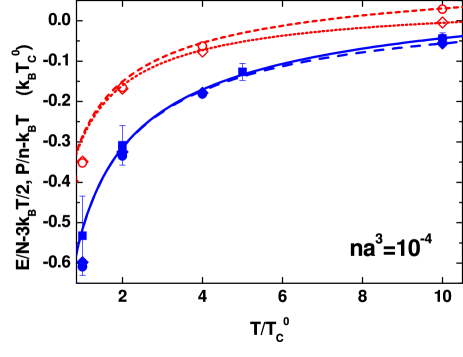
Figure 2: (color online). Energy per particle and pressure of a Bose gas in the normal phase as a function of the temperature for $na^{3}=10^{-4}$. Same notation as in Fig. 1, except for the results of the energy for the NP potential, shown here as squares (blue online).

Figure 3: (color online). Energy per particle and pressure of a Bose gas in the normal phase as a function of the temperature for $na^{3}=10^{-2}$. Same notation as in Figs. 1 and 2.

At high temperatures $n\lambda_{T}^{3}\ll 1$, where $\lambda_{T}=\sqrt{2\pi\hbar^{2}/mk_{B}T}$ is the thermal wave length, the equation of state of the gas can be calculated from the virial expansion

$$\frac{PV}{Nk_{B}T}=1+a_{2}(T)n\lambda_{T}^{3}+...\;,$$ (19)

where we considered only the contribution arising from the second virial coefficient $a_{2}(T)$. The corresponding virial expansion of the energy per particle can be calculated using standard thermodynamic relations and one finds Landau1

$$\frac{E}{N}=\frac{3}{2}k_{B}T\left(1+a_{2}(T)n\lambda_{T}^{3}+...\right)\;.$$ (20)

For a non-interacting Bose gas the second virial coefficient can be promptly calculated with the result $a_{2}^{0}=-1/\sqrt{2^{5}}$, determined by statistical effects. For a gas of particles interacting through a repulsive interatomic potential $a_{2}(T)$ can be calculated through a summation over partial waves Pathria

$$a_{2}(T)=a_{2}^{0} - \frac{\sqrt{8}}{\pi}\sum_{\ell=0,2,4,...}(2\ell+1)$$ (21)

$$\times \int_{0}^{\infty}dke^{-\hbar^{2}k^{2}/mk_{B}T}\frac{\partial\delta_{\ell}(k)}{\partial k}\;.$$

For bosons, the sum in Eq. (21) only includes even partial waves. The $\ell$-th partial-wave phase shift $\delta_{\ell}(k)$ in the above equation is obtained from the solution of the Schrödinger equation (16) for the given potential $V(r)$ with the boundary condition (17). If the thermal wave length is much larger than the range of the potential, $\lambda_{T}\gg R_{0}$, one obtains, to lowest order, the following result

$$a_{2}(T)-a_{2}^{0}=2\frac{a}{\lambda_{T}}+...\;,$$ (22)

which only depends on the scattering length $a$.

In Figs. 1-3, we present the PIMC results for the energy per particle $E/N$ and pressure $P$ in the normal phase ($T>T_{c}$) for three different values of the gas parameter: $na^{3}=10^{-6}$ (Fig. 1), $na^{3}=10^{-4}$ (Fig. 2) and $na^{3}=10^{-2}$ (Fig. 3). In order to emphasize the deviations from the classical results we plot the quantities $E/N-3k_{B}T/2$ and $P/n-k_{B}T$. We also plot the corresponding virial expansions from Eqs. (19),(20) with the second virial coefficient $a_{2}(T)$ calculated using Eq. (21) for the HS and SS potentials. For the smallest value of the interaction strength, $na^{3}=10^{-6}$, we find very good agreement between the HS and SS results and with the virial expansions down to temperatures close to the transition temperature. At $na^{3}=10^{-4}$, the virial expansion still provides a good approximation in the whole temperature regime and deviations are found only at the lowest temperatures $T\sim T_{c}^{0}$. On the other hand, universality is maintained only for low $T$ since differences between the HS and SS potentials start to become visible for temperatures $T/T_{c}^{0}\gtrsim 4$. Finally, for the largest interaction strength $na^{3}=10^{-2}$, the universal behavior fixed by the scattering length $a$ is lost in the whole temperature range. For the HS potential, agreement with the virial expansion is found only at the largest temperature. Concerning the results for the NP potential obtained with the CA approximation, notice that already for $na^{3}=10^{-4}$ the statistical uncertainty is significantly larger than the one corresponding to results for the HS and SS potentials obtained using the PPA. This fact is due to the large separation in scale between the range of interactions and the mean interparticle distance which occurs in dilute systems. For very small values of the gas parameter $na^{3}$ the algorithm based on the PPA, which is constructed from the exact solution of the two-body problem, converges much faster than the one based on the CA. For example, at $T=2T_{c}^{0}$ and $na^{3}=10^{-4}$, the calculation for the NP potential has been performed using up to $M=200$ beads in contrast to only $M=12$ in the case of the HS and SS potentials. For the smallest value of the interaction strength, $na^{3}=10^{-6}$, and especially for temperatures below the transition temperature, the calculation using the CA approach becomes much more computationally demanding due to the large number of beads required.

III.2 Superfluid phase

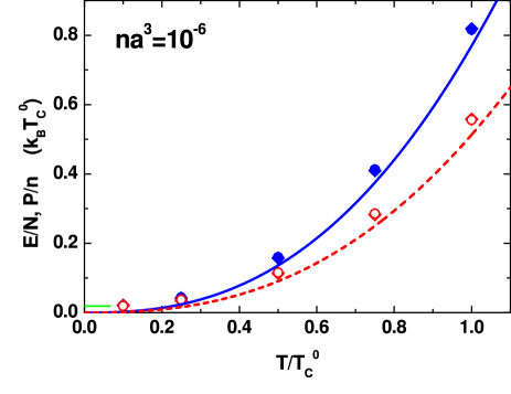
Figure 4: (color online). Energy per particle and pressure of a Bose gas in the superfluid phase as a function of temperature. The gas parameter is $na^{3}=10^{-6}$. Solid symbols (blue online) refer to $E/N$: HS potential (circles), SS potential (diamonds). Open symbols (red online) refer to $P/n$: HS potential (circles), SS potential (diamonds). Statistical error bars are smaller than the size of the symbols. The horizontal bar (green online) corresponds to the ground-state energy per particle $E_{0}/N$ of a HS gas calculated using DMC. The lines correspond to a non-interacting gas: the solid line (blue online) refers to the energy per particle and the dashed line (red online) to the pressure.

Figure 5: (color online). Energy per particle and pressure of a Bose gas in the superfluid phase as a function of the temperature for $na^{3}=10^{-4}$. Same notation as in Fig. 4, except for the results of the energy for the NP potential, shown here as squares (blue online).

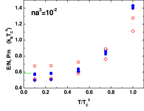
Figure 6: (color online). Energy per particle and pressure of a Bose gas in the superfluid phase as a function of the temperature for $na^{3}=10^{-2}$. Same notation as in Figs. 4 and 5.

The determination of the transition temperature from the equation of state is very delicate as it involves a slight change of the energy vs. $T$ dependence at $T_{c}$. Its precise determination would require the calculation of the specific heat. Other observables, like the superfluid density and the condensate fraction, give a direct signature of the transition 3dhomo1 ; 3dhomo2 . The most reliable results so far give the following shift of the transition temperature $T_{c}$ 3dhomo2

$$\frac{T_{c}-T_{c}^{0}}{T_{c}^{0}}=(1.29\pm 0.05)(na^{3})^{1/3}\;,$$ (23)

holding for very small values of the gas parameter. For the values of $na^{3}$ used in the present study, the above equation yields estimates of $T_{c}$ ranging from 1% to 30% above $T_{c}^{0}$. We are not interested here in the calculation of $T_{c}$ and the focus is only on the precise determination of the equation of state.

In Figs. 4-6, we show results for $E/N$ and $P/n$ in the superfluid phase ($T<T_{c}$) for the three values of the gas parameter: $na^{3}=10^{-6}$ (Fig. 4), $na^{3}=10^{-4}$ (Fig. 5) and $na^{3}=10^{-2}$ (Fig. 6). To emphasize the effects of interactions in Figs. 4 and 5 we also plot the energy per particle and the pressure of an ideal Bose gas. For $na^{3}=10^{-6}$ and $na^{3}=10^{-4}$ we see very small differences between the results of the HS and SS potentials (notice the large statistical uncertainty in the results of the NP potential at $na^{3}=10^{-4}$). For the largest value of $na^{3}$ we still find good agreement between the results of the HS and NP potential, while significant differences are found between the HS and SS potential. At very low temperatures, the PIMC results agree with the ground-state energy per particle $E_{0}/N$ obtained for the HS potential using the DMC method US . For the three values of the gas parameter used in the present study the results are (in units of $k_{B}T_{c}^{0}$): $E_{0}/N=0.01905(2)$ at $na^{3}=10^{-6}$, $E_{0}/N=0.09185(8)$ at $na^{3}=10^{-4}$, and $E_{0}/N=0.5840(4)$ at $na^{3}=10^{-2}$.

The PIMC results for $E/N$ and $P/n$ obtained using the HS and SS potential at the various temperatures and for the three values of $na^{3}$ are reported in Tables LABEL:tab1, LABEL:tab2. Finite size effects are relevant only in the simulations performed at $T=T_{c}^{0}$ because of the vicinity to the critical point. For example, in the case of the HS potential at $na^{3}=10^{-4}$ we find for this temperature the result: $E/(Nk_{B}T_{c}^{0})=0.935(7)$ with $N=64$ and $E/(Nk_{B}T_{c}^{0})=0.891(13)$ with $N=1024$.

IV Conclusions

In conclusion, we have carried out using exact PIMC methods a precision calculation of the equation of state of an interacting Bose gas as a function of temperature and interaction strength. The universal character of the equation of state at low temperatures and small values of the gas parameter is pointed out by performing simulations with different interatomic model potentials. Above the transition temperature we compare our results for energy and pressure with the high-temperature expansion based on the second virial coefficient. The inclusion of tables for both energy and pressure is intended as a reference for future studies of the thermodynamic properties of interacting Bose gases.

Table 1: Energy per particle $E/N$ (in units of $k_{B}T_{c}^{0}$) for the HS and SS potential and different values of the gas parameter $na^{3}=10^{-6}$, 10^-4, 10^-2. In parenthesis we give the statistical errors.

	$E/N$ $\;\;\;\;\;\;(k_{B}T_{c}^{0}$)
	$na^{3}=10^{-6}$		$na^{3}=10^{-4}$		$na^{3}=10^{-2}$
$T/T_{c}^{0}$	$HS$	$SS$	$HS$	$SS$	$HS$	$SS$
0.10	0.022(1)	0.021(1)	0.093(1)	0.093(1)	0.577(5)	0.499(1)
0.25	0.043(2)	0.042(1)	0.111(2)	0.110(1)	0.586(4)	0.506(1)
0.50	0.160(4)	0.158(3)	0.214(4)	0.218(4)	0.639(5)	0.606(4)
0.75	0.402(5)	0.409(7)	0.475(14)	0.464(13)	0.856(13)	0.885(13)
1.00	0.816(10)	0.819(6)	0.891(13)	0.902(15)	1.398(10)	1.431(18)
2.00	2.540(6)	2.541(5)	2.665(13)	2.675(8)	3.328(4)	3.090(3)
4.00	5.694(5)	5.692(5)	5.818(7)	5.821(5)	6.458(3)	6.196(3)
10.0	14.817(5)	14.821(5)	14.956(4)	14.943(3)	15.527(6)	15.312(4)
20.0	29.885(5)	29.880(5)	30.023(4)	29.989(2)	30.615(11)	30.374(4)

Table 2: Pressure $P/n$ (in units of $k_{B}T_{c}^{0}$) for the HS and SS potential and different values of the gas parameter $na^{3}=10^{-6}$, 10^-4, 10^-2. In parenthesis we give the statistical errors.

	$P/n$ $\;\;\;\;\;\;(k_{B}T_{c}^{0}$)
	$na^{3}=10^{-6}$		$na^{3}=10^{-4}$		$na^{3}=10^{-2}$
$T/T_{c}^{0}$	$HS$	$SS$	$HS$	$SS$	$HS$	$SS$
0.10	0.021(1)	0.021(1)	0.095(1)	0.094(1)	0.676(6)	0.514(1)
0.25	0.037(2)	0.035(1)	0.107(2)	0.106(1)	0.680(4)	0.520(2)
0.50	0.116(3)	0.114(2)	0.183(4)	0.180(4)	0.724(4)	0.582(3)
0.75	0.285(5)	0.283(5)	0.362(9)	0.353(9)	0.890(8)	0.761(8)
1.00	0.556(7)	0.558(4)	0.648(10)	0.651(10)	1.276(8)	1.113(12)
2.00	1.708(4)	1.706(3)	1.835(9)	1.832(5)	2.572(3)	2.223(3)
4.00	3.808(4)	3.807(3)	3.937(5)	3.924(4)	4.716(4)	4.308(3)
10.0	9.891(4)	9.893(3)	10.028(3)	9.995(2)	10.954(8)	10.378(3)
20.0	19.936(3)	19.932(3)	20.075(4)	20.024(2)	21.335(10)	20.416(3)

References

- (1) M.H. Anderson et al., Science 269, 198 (1995); K.B. Davis et al., Phys. Rev. Lett. 75, 3969 (1995); C.C. Bradley et al., Phys. Rev. Lett. 75, 1687 (1995).
- (2) L.P. Pitaevskii and S. Stringari, Bose-Einstein Condensation, (Clarendon Press, Oxford, 2003).
- (3) F. Dalfovo, S. Giorgini, L.P. Pitaevskii and S. Stringari, Rev. Mod. Phys. 71, 463 (1999).
- (4) W. Krauth, Phys. Rev. Lett. 77, 3695 (1996); M. Holzmann, W. Krauth and M. Naraschewski, Phys. Rev. A 59, 2956 (1999); M. Holzmann and Y. Castin, Eur. Phys. J. D 7, 425 (1999).
- (5) S. Heinrichs, W.J. Mullin, J. Low Temp. Phys. 113, 231 (1998); K. Nho and D. Blume, Phys. Rev. Lett. 95, 193601 (2005).
- (6) P. Grüter, D.M. Ceperley and F. Laloë, Phys. Rev. Lett. 79, 3549 (1997); M. Holzmann and W. Krauth, Phys. Rev. Lett. 83, 2687 (1999).
- (7) V. A. Kashurnikov, N.V. Prokof’ev and B.V. Svistunov, Phys. Rev. Lett. 87, 120402 (2001); N. Prokof’ev, O. Ruebenacker and B. Svistunov, Phys. Rev. A 69, 053625 (2004); K. Nho and D.P. Landau, Phys. Rev. A 70, 053614 (2004).
- (8) N. Prokof’ev, O. Ruebenacker and B. Svistunov, Phys. Rev. Lett. 87, 270402 (2001).
- (9) S. Giorgini, J. Boronat and J. Casulleras, Phys. Rev. A 60, 5129 (1999).
- (10) L.D. Landau and E.M. Lifshitz, Quantum Mechanics (Non-relativistic Theory) (Pergamon Press, Oxford, 1977), pag. 550.
- (11) E.L. Pollock and D.M. Ceperley, Phys. Rev. B 30, 2555 (1984); ibid. 36, 8343 (1987); D.M. Ceperley, Rev. Mod. Phys. 67, 1601 (1995).
- (12) H.F. Trotter, Proc. Am. Math. Soc. 10, 545 (1959).
- (13) L. Brualla, K. Sakkos, J. Boronat and J. Casulleras, J. Chem. Phys. 121, 636 (2004).
- (14) S. A. Chin and C. R. Chen, J. Chem. Phys. 117, 1409 (2002).
- (15) K. Sakkos, J. Casulleras, and J. Boronat, to be published.
- (16) J. Cao and B.J. Berne, J. Chem. Phys. 97, 2382 (1992).
- (17) L.D. Landau and E.M. Lifshitz, Statistical Physics Part 1 (3rd edition) (Pergamon Press, Oxford, 1980), Ch. 7.
- (18) R.K. Pathria, Statistical Mechanics 2nd edition (Butterworth-Heinemann, Oxford, 1996), pag. 252-253.