Structural and dynamical heterogeneity in a glass forming liquid

Abstract

We use the “isoconfigurational ensemble” [Phys. Rev. Lett. 93, 135701 (2004)] to analyze both dynamical and structural properties in simulations of a glass forming molecular liquid. We show that spatially correlated clusters of low potential energy molecules are observable on the time scale of structural relaxation, despite the absence of spatial correlations of potential energy in the instantaneous structure of the system. We find that these structural heterogeneities correlate with dynamical heterogeneities in the form of clusters of low molecular mobility.

Over the last decade, the identification and study of dynamic heterogeneity (DH), especially in computer simulations, has added an important new dimension to our understanding of complex relaxation in glass forming liquids E00 ; G00 . DH refers to the emergence and growth of spatially correlated domains of mobile and immobile molecules as temperature $T$ approaches the glass transition temperature $T_{g}$. A question that dominates research on DH concerns its connection to the structure of the liquid: What local configurational properties influence whether a given molecule is mobile or immobile?

Recent work by Widmer-Cooper, Harrowell and Fynewever CHF04 has shown conclusively that a structure-dynamics connection must exist at the molecular level. To do so, they use an “isoconfigurational (IC) ensemble” CHF04 ; CH05 ; DH03 , a set of microcanonical molecular dynamics (MD) trajectories in which each run starts from the same initial equilibrium configuration, but with molecular momenta chosen randomly accordingly to a Maxwell-Boltzmann distribution. The result is a set of trajectories lying on the same energy surface, and evolving away from their common initial point in configuration space. They then define and evaluate the “dynamic propensity”: the average, in the IC ensemble, of the squared displacement of a molecule at a time comparable to the structural relaxation time. They show that DH is observed in this approach, in the form of increasing spatial correlations of the dynamic propensities in a glass forming liquid as $T\to T_{g}$. Since the influence of the initial momenta is averaged over, the observed spatial correlations must be configurational in origin.

The strength of Ref. CHF04 is that it exposed the features of DH that are structural in origin, without needing to determine what structural properties are responsible. Other studies have worked towards explicitly identifying structural correlators to dynamics. A number of works over the past decades have identified relationships between average structural properties (especially free volume and measures of symmetry in the local molecular environment) and bulk dynamics; see e.g. Refs. SNR81 ; H82 ; JA88 ; Starr02 . More recently, several studies have sought a correlation at the microscopic level, e.g. between local free volume and local mobility, with more success in some systems LT06 ; JP05 than in others CSW05 . A notable absence of correlation between the local volume and the local Debye-Waller factor has been reported recently CHcm . Insights have also been realized using local measures of symmetry to elucidate local mobility, e.g. icosohedral order DSZ02 ; JP05 ; or the recent work of Shintani and Tanaka in which less mobile regions were shown to correlate well to structured, crystal-like domains ST06 . Recently, the local Debye-Waller factor has been shown to correlate to the dynamic propensity CH06 , firmly establishing the connection between local dynamics at short and long times.

Notably absent from the list of local structural quantities that correlate well to local dynamics is the potential energy. It has been shown that a molecule with a low potential energy will be less mobile, on average, than one with a high potential energy D99 . However, the variance around this average trend is comparable to or larger than the trend itself, making it impossible to predict what a given molecule will do based on its potential energy. Careful time averaging LT06 and the use of inherent structures CH06 has been shown to yield little gain in correlation. This is both perplexing and disappointing. Perplexing since we know that the average potential energy strongly influences the average dynamics of the system NS04 . And disappointing because the potential energy is a natural observable to correlate to dynamics, especially given the interest in the analysis of glass-forming systems using the potential energy landscape Wales .

In this Letter, by expanding the application of the IC ensemble to structural quantities, we show that it is possible to identify heterogeneities of the potential energy that correlate well to dynamic heterogeneities, in a liquid where no useful correlation is discernible from the instantaneous properties of the system. Our work shows that emergent “structural heterogeneities”, that develop in tandem with dynamic heterogeneities, exist and can be observed in a glass forming liquid.

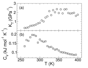
Figure 1: (a) $K_{T}$ and (b) $C_{V}$ as a function of $T$ along the $\rho=0.83$ g/cm³ isochore. Data are derived from the simulations described in Ref. PSS05 .

Our results are based on molecular dynamics simulations of $N=1728$ water molecules interacting via the ST2 pair potential st2 . Much is known about this simulation model, both in terms of thermodynamic and transport behavior, making it a good candidate for a detailed analysis of structure-dynamics relationships in a model 3D molecular liquid SPES97 ; PG99 ; PSS05 ; BPScm . We study three $T$ (350, 290 and 270 K) all at density $\rho=0.83$ g/cm³. At this $\rho$, the hydrogen bond network in this water model is more prominent than at other $\rho$, suggesting that local energetics may have a particularly strong influence on dynamics. This $\rho$ is also a convenient choice because the isothermal compressibility $K_{T}$ (which is related to the strength of static density fluctuations) is decreasing with $T$ (Fig. 1). This ensures that any DH that emerges as $T$ decreases will not be due to the growth of conventional density fluctuations. At the same time, we note that the isochoric specific heat $C_{V}$ (and hence the magnitude of fluctuations of the system energy) is increasing to a maximum, so spatial variations of potential energy may be occurring. These conditions therefore provide a promising regime in which to seek connections between energy and dynamics at the molecular level.

In all our simulations, molecular interactions are cut off at a distance of $0.78$ nm, and effects of those at longer range are approximated via the reaction field method. All simulations have constant $N$ and volume $V$, and use a 1 fs time step. At each $T$, we first conduct a standard MD run where $T$ is maintained near the desired value using the method of Berendsen, et al beren . To ensure equilibration, these runs are carried out for twice the time required for the mean squared displacement to reach 1 nm². We then use the configuration at the end of the equilibration run as the initial configuration for generating $M=1000$ runs of an IC ensemble. Note that both the linear and angular momentum of each molecule is randomized, using the Maxwell-Boltzmann distribution appropriate to the $T$ of the initial configuration. Each run is carried out in the microcanonical ensemble for a time $t=308$ ps (350 and 290 K) or $937$ ps (270 K).

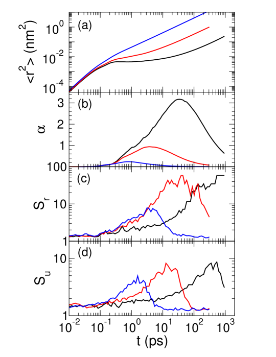
Figure 2: (a) Mean squared displacement $\langle r^{2}\rangle$, (b) non-Gaussian parameter $\alpha$, (c) mean cluster size for least mobile molecules, $S_{r}$, and (d) mean cluster size for tightly bound molecules, $S_{u}$, all as a function of $t$. From left to right in (a), the curves are for $T=350$, 290 and 270 K. In (b-d), the curve with the left-most maximum is $T=350$ K, the middle maximum is $290$ K, and the right-most is $270$ K.

Let $r^{2}(i,k,t)$ be the squared displacement of the O atom of molecule $i$ at time $t$ in run $k$ of an IC ensemble. The system-averaged and IC-ensemble-averaged mean squared displacement, $\langle r^{2}\rangle=(NM)^{-1}\sum_{i=1}^{N}\sum_{k=1}^{M}r^{2}(i,k,t)$, and non-Gaussian parameter, $\alpha=[(3\langle r^{4}\rangle)/(5\langle r^{2}\rangle^{2})]-1$ are shown in Fig. 2. Both show the characteristic pattern of a glass forming liquid in which DH occurs. $\langle r^{2}\rangle$ develops a plateau at low $T$ indicating the onset of molecular caging, and $\alpha$ displays an increasingly prominent maximum as $T$ decreases. We have checked that the curves in Figs. 2(a-b) are, at large $t$, within error of those found in a conventional approach, where an average is taken over multiple time origins of a single, long MD run. This suggests that the particular initial configurations chosen are at least approximately representative of the equilibrium behavior.

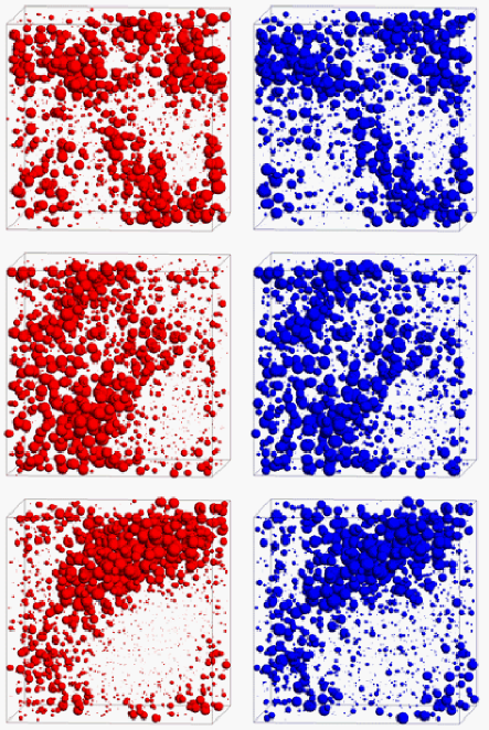
Figure 3: Dynamical heterogeneity (left panels) and structural heterogeneity (right panels) in the initial configuration at $T=350$ K (top panels), 290 K (middle panels) and 270 K (bottom panels). To make each panel, the values of $\langle r_{i}^{2}\rangle_{\rm ic}$ (or $\langle u_{i}\rangle_{\rm ic}$), evaluated at the time of the maximum of $S_{u}$, are assigned to each molecule in the initial configuration. These values are sorted and assigned an integer rank $R_{i}$ from 1 to $N$, from smallest to largest. Each O atom is then plotted as a sphere of radius $R_{\rm min}\exp\{[(R_{i}-N)/(1-N)]\log(R_{\rm max}/R_{\rm min})\}$, where $R_{\rm max}=0.14$ nm and $R_{\rm min}=0.004$ nm. The result represents the rank of $\langle r_{i}^{2}\rangle_{\rm ic}$ or $\langle u_{i}\rangle_{\rm ic}$ on an exponential scale, such that the largest spheres on the left represent the least mobile molecules, and the largest on the right the most tightly bound. Note that hydrogen atoms are not shown.

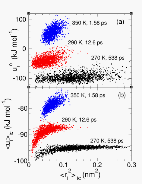
Figure 4: (a) $u_{i}^{\circ}$ and (b) $\langle u_{i}\rangle_{\rm ic}$, both versus $\langle r_{i}^{2}\rangle_{\rm ic}$ at each $T$. The times indicated, at which $\langle u_{i}\rangle_{\rm ic}$ and $\langle r_{i}^{2}\rangle_{\rm ic}$ are evaluated, correspond to the maxima of $S_{u}$. To ease comparison, in (a) the cloud for $290$ K has been shifted upward by $50$ kJ/mol, and that for $350$ K by 130 kJ/mol; in (b) the cloud for $350$ K has been shifted down by 4 kJ/mol.

The dynamic propensity of each molecule is the value of $\langle r_{i}^{2}\rangle_{\rm ic}=M^{-1}\sum_{k=1}^{M}r^{2}(i,k,t)$ when $t$ is on the order of the structural relaxation time CHF04 . It measures the propensity for molecule $i$ to undergo a given displacement, given its starting point in the initial configuration, rather than indicating what the molecule will do in any particular run. Here, we extend the use of the IC ensemble to study structural properties as well as dynamics. We focus on $u(i,k,t)$, the contribution of molecule $i$ to the instantaneous potential energy of the system at time $t$ in run $k$ of an IC ensemble. Specifically, $u_{i}=\sum_{j=1}^{N}\phi_{ij}$, where $\phi_{ij}$ is the pair potential energy of molecules $i$ and $j$. Analogous to $\langle r_{i}^{2}\rangle_{\rm ic}$ we define $\langle u_{i}\rangle_{\rm ic}=M^{-1}\sum_{k=1}^{M}u(i,k,t)$. At a fixed $t$, $\langle u_{i}\rangle_{\rm ic}$ measures the propensity of molecule $i$ to have a given value of the potential energy, given its starting point in the initial configuration.

First we test for the occurrence of DH, by evaluating $\langle r_{i}^{2}\rangle_{\rm ic}$ for each molecule as a function of $t$, and examining the spatial arrangement of this quantity via a cluster analysis VG04 ; Starr06 . For reasons that will become clear below, we focus on the least mobile molecules, specifically the subset having the lowest $10\%$ of $\langle r_{i}^{2}\rangle_{\rm ic}$ values. Clusters are defined by the rule that two molecules of this subset that are also within $0.35$ nm of one another (the position of the first minimum of the O-O radial distribution function) in the initial configuration are assigned to the same cluster. The number-averaged mean cluster size $S_{r}$ is then found from $(1/N_{c})\sum_{n}nC(n)$, where $C(n)$ is the number of clusters of size $n$, and $N_{c}$ is the total number of clusters. Fig. 2(c) shows the $t$ dependence of $S_{r}$ at each $T$. At small $t$, $S_{r}$ has a value consistent with a random choice of $10\%$ of the molecules, approximately $S_{r}=1.27$, indicating no spatial correlations in $\langle r_{i}^{2}\rangle_{\rm ic}$. However, at intermediate times corresponding to the onset of structural relaxation, a maximum occurs, indicating significant clustering of the least mobile molecules. At large $t$, $S_{r}$ begins its return to the uncorrelated value, and the DH dissolves. The morphology of the DH observed near the maxima in Fig. 2(c) is illustrated in the left panels of Fig. 3. The correlated domains of larger spheres in Fig. 3 indicate the locations of the large clusters that generate the maxima in Fig. 2(c).

We then carry out exactly the same analysis, but using the lowest $10\%$ of $\langle u_{i}\rangle_{\rm ic}$ values; this selects the subset of molecules with the greatest propensity to be “tightly bound.” The mean cluster size for this subset, $S_{u}$, shows a similar behavior to $S_{r}$ [Fig. 2(d)]. Note that in the limit $t\to 0$, we have $\langle u_{i}\rangle_{\rm ic}\to u_{i}^{\circ}$, where $u_{i}^{\circ}$ is the instantaneous potential energy of each molecule in the initial configuration. The behavior of $S_{u}$ at small $t$ confirms that $u_{i}^{\circ}$ shows essentially no spatial correlation at any $T$. And yet, on the same time scale as the signature of DH is observed in $S_{r}$, a maximum also occurs in $S_{u}$. The spatial correlations of molecular potential energies (i.e. structural heterogeneities) that generate the maxima in $S_{u}$ are illustrated in Fig. 3. The morphology of the two types of heterogeneity shown in Fig. 3 is strikingly similar: there is a clear correlation between regions with a propensity to be the least mobile, and a propensity to be tightly bound. It is worth bearing in mind that these two types of heterogeneity are defined independently. Neither the time scale on which the structural heterogeneity occurs, nor the definition of the structural clusters depends on dynamical information.

The absence of a useful correlation between $u_{i}^{\circ}$ and the dynamic propensity is demonstrated by a scatter plot of $u_{i}^{\circ}$ against $\langle r_{i}^{2}\rangle_{\rm ic}$, evaluated at the time of the maximum of $S_{u}$ at each $T$ [Fig. 4(a)]. The best correlation is found at high $T$, but even here some molecules in the lowest $10\%$ of $u_{i}^{\circ}$ have values of $\langle r_{i}^{2}\rangle_{\rm ic}$ comparable or even larger than the mean of $\langle r_{i}^{2}\rangle_{\rm ic}$. At lower $T$ the correlation only gets worse: molecules with the lowest values of $u_{i}^{\circ}$ are found across the entire spectrum of $\langle r_{i}^{2}\rangle_{\rm ic}$ values. We have also tested if the correlation improves if we replace $u_{i}^{\circ}$ in Fig. 4(a) with its value in the inherent structure of the initial configuration, but it does not.

Fig. 4(b) shows a scatter plot of $\langle u_{i}\rangle_{\rm ic}$ versus $\langle r_{i}^{2}\rangle_{\rm ic}$ at the time of the maximum of $S_{u}$ at each $T$. Here we see the reason why we have focussed on the least mobile and most tightly bound molecules: it is at the lower end of these scatter plots that the points are most easily distinguished from the overall population. In contrast, the correlation between the most mobile and least tightly bound molecules is little improved over that in Fig. 4(a). We have also examined the clusters formed by the $10\%$ most mobile and least tightly bound subsets of molecules. The most mobile molecules also form clusters at intermediate times, although the strength of the effect is weaker than for the least mobile molecules. Interestingly, the least tightly bound subset shows a decreasing tendency to cluster as $T$ decreases, with the maximum in $S_{u}$ becoming difficult to discern at the lowest $T$. Whether this is a generic behavior, or a feature of this particular network-forming liquid requires further research, which is currently underway. One possibility is that molecular hopping is emerging as an important mode of transport at low $T$, which might weaken the energy-dynamics correlation for the most mobile molecules PG99 .

We can therefore make the following statements about the relationship of local potential energy and local dynamics in this system: Despite the absence of a correlation between the instantaneous potential energy of a molecule and its subsequent displacement, a molecule that has a propensity to be tightly bound (as evaluated within the IC ensemble) also has a propensity to be among the least mobile. On the other hand, a propensity to be mobile and a propensity to be loosely bound do not correlate at low $T$, indicating that other factors are controlling dynamics at this end of the spectrum. The IC ensemble thus makes possible a dissection of the energy-dynamics relationship, under conditions where no conclusions can be drawn from instantaneous structural information. The approach also exposes the morphology of the structural heterogeneity present in a single instantaneous configuration. As Ref. CHF04 first showed, averaging over the IC ensemble therefore acts as a powerful amplifier of the subtle configurational signal that must exist instantaneously, but which is overwhelmed by the “noise” imposed by molecular momenta. While we have only addressed the behavior of the potential energy in this work, we expect that valuable information concerning many supercooled liquids can be extracted from a wide range of configurational quantities (e.g local volume, local symmetry) when evaluated at the local level in the IC ensemble.

Our work also demonstrates that the emergence and growth of heterogeneity in a glass forming liquid is not solely a dynamical phenomena, but also structural, and that the two types of heterogeneity can be analyzed within the same framework by using the IC ensemble. In particular, we note that the size of the structural and dynamical heterogeneities observed here are approaching the system size at our lowest $T$. It may be that the ability of the IC ensemble to discern subtle spatial correlations will help clarify the nature of the growing length scales of dynamic and structural heterogeneity as $T\to T_{g}$.

We thank R. Bowles, P. Kusalik, and F. Starr for useful input; F. Sciortino for the code to find the inherent structures of the initial configurations; and especially P. Harrowell for stimulating our interest in this topic. Financial and computing support was provided by ACEnet, NSERC, AIF, CFI and the CRC program.

References

- (1) M.D. Ediger, Annu. Rev. Phys. Chem. 51, 99 (2000).
- (2) S.C. Glotzer, Journal of Non-Crystalline Solids 274, 342 (2000).
- (3) A. Widmer-Cooper, P. Harrowell and H. Fynewever, Phys. Rev. Lett. 93, 135701 (2004).
- (4) A. Widmer-Cooper and P. Harrowell, J. Phys. Condens. Matter 17, S4025 (2005).
- (5) B. Doliwa and A. Heuer, Phys. Rev. Lett. 91, 235501 (2003); Phys. Rev. E 67, 031506 (2003).
- (6) P.J. Steinhardt, D.R. Nelson and M. Ronchetti, Phys. Rev. Lett. 47, 1297 (1981).
- (7) Y. Hiwatari, J. Chem. Phys. 76, 5502 (1982).
- (8) H. Jonsson and H.C. Andersen, Phys. Rev. Lett. 60, 2295 (1988).
- (9) F.W. Starr, S. Sastry, J.F. Douglas and S.C. Glotzer, Phys. Rev. Lett. 89, 125501 (2002).
- (10) I. Ladadwa and H. Teichler, Phys. Rev. E 73, 031501 (2006).
- (11) T.S. Jain and J.J. de Pablo, J. Chem. Phys. 122, 174515 (2005).
- (12) J.C. Conrad, F.W. Starr and D.A. Weitz, J. Phys. Chem. B 109, 21235 (2005).
- (13) A. Widmer-Cooper and P. Harrowell, cond-mat/0511690.
- (14) M. Dzugutov, S.I. Simdyankin and F.H.M. Zetterling, Phys. Rev. Lett. 89, 195701 (2002).
- (15) H. Shintani and H. Tanaka, Nature Physics 2, 200 (2006).
- (16) A. Widmer-Cooper and P. Harrowell, Phys. Rev. Lett. 96, 185701 (2006).
- (17) C. Donati, S.C. Glotzer, P.H. Poole, W. Kob and S.J. Plimpton, Phys. Rev. E 60, 3107 (1999).
- (18) E. La Nave and F. Sciortino, J. Phys. Chem. B 108, 19663 (2004).
- (19) D. Wales, “Energy Landscapes”, Cambridge University Press, New York (2003).
- (20) F.H. Stillinger and A. Rahman, J. Chem. Phys. 60, 1545 (1974).
- (21) F. Sciortino, P.H. Poole, U. Essmann and H.E. Stanley, Phys. Rev. E 55, 727 (1997).
- (22) D. Paschek and A. Geiger, J. Phys. Chem. B 103, 4139 (1999).
- (23) P.H. Poole, I. Saika-Voivod and F. Sciortino, J. Phys. Condens. Matter 17, L431 (2005).
- (24) S.R. Becker, P.H. Poole and F.W. Starr, Phys. Rev. Lett., in press (2006).
- (25) H.J.C. Berendsen, et al., J. Chem. Phys. 81, 3684 (1984).
- (26) M. Vogel and S.C. Glotzer, Phys. Rev. Lett. 92, 255901 (2004); Phys. Rev. E 70, 061504 (2004).
- (27) M.G. Mazza, N. Giovambattista, F.W. Starr and H.E. Stanley, Phys. Rev. Lett. 96, 057803 (2006).