Ordering dynamics in Type-II superconductors

Abstract

We use analytic and numerical methods to analyze the dynamics of vortices following the quench of a Type-II superconductor under the application of an external magnetic field. In three dimensions, in the absence of a field, the spacing between vortices scales with time $t$ with an exponent $\phi=0.414\pm 0.01$, In a thin sheet of superconductor, the scaling exponent is $\phi=0.294\pm 0.01$. When an external magnetic field $h$ is applied, the vortices are confined with respect to the length scale of the Abrikosov lattice, leading to a crossover between the power-law scaling length scale and the lattice length scale. From this we suggest a one-parameter scaling of $\dot{r}$ with $h$ and $r$ that is consistent with numerical data.

I INTRODUCTION

Systems with continuous symmetries exhibit interesting time-dependent scaling behavior following a quench, due to the dynamics of topological defects Toyoki and Honda (1987); Mondello and Goldenfeld (1990, 1992); Liu et al. (1991); Frahm et al. (1991); Blundell and Bray (1992); Bray (2002). Physical realizations include superfluid He⁴ and He³, Bose-Einstein condensates, liquid crystals, and models of cosmic strings - defects produced during phase transitions in the early universe Kibble (1976). In this paper, we investigate the effect of topological defects in the approach to equilibrium of Type-II superconductors and examine the consequences to the dynamics of the presence of a gauge field Liu et al. (1991); Frahm et al. (1991).

Following a quench from the normal phase, a Type-II superconductor is threaded by a series of vortex cores (which are line defects) due to fluctuations that had existed in the normal phase. Over time, these vortex cores interact through local and long-range forces. In the absence of an external field, the number of vortices decreases with time, giving rise to a characteristic length-scale $r(t)$ that coarsens with time $t$, generically with a power law whose exponent we denote by $\phi$.

A variety of predictions have been made for the scaling of $r(t)$ by treating the problem with various reduced models. A first approximation to the scaling of defect spacing can be found by solving the equations of motion for a pair of defects. For local interactions between defects the strongest contribution is from the immediate neighbor, and the effect of the remainder of the defects is to distribute momentum via long-wavelength modes throughout the bulk, leading to over-damped dissipative dynamics.

We can estimate the dynamics in this approximation from the potential energy of interaction of a defect pair Bray (2002). This will play a role in determining how clusters of defects expand, which in turn determines the time-dependence of such quantities as the total defect volume, spacing between defects, and defect correlation functions. If the interaction is purely from the stress induced by the topological defect in the continuously symmetric field then the potential will be of the form $V(r)\propto\log(r/\xi)$ for both point defects in 2D and line defects in 3D, leading to a force of the form $F(r)\propto(r/\xi)^{-1}$. Here we have introduced a characteristic length scale $\xi$, which is of order the vortex core size. Similarly, a point defect in 3D would experience a potential $V(r)\propto(r/\xi)^{-1}$ and a force proportional to $(r/\xi)^{-2}$.

In overdamped dynamics, the time-derivative $\dot{r}(t)$ is proportional to the force of interaction between two defects. For the $r^{-1}$ force appropriate for line defects in three dimensions, we find that when $r(t)$ is much greater than the initial inter-vortex distance, $r\propto t^{\phi}$ with the dynamical exponent $\phi=1/2$.

In a superconductor, vortices are surrounded by loops of superconducting currents, matched to a magnetic field which threads the vortices. As a result, there are magnetic interactions which depend on the geometry and dimension of the system in addition to the direct interaction of the topological defects. In the bulk of a superconductor the field is screened and the force law is exponentially decaying with the distance, leading to a logarithmic scaling of the inter-vortex distance with time. In a thin film of superconducting material (which will be referred to as the 2DF system), where the magnetic flux is allowed to penetrate into the third dimension, the force law is that of point interactions in three dimensional space, and results in a power law scaling of $r(t)$ with an exponent $\phi=1/3$.

These exponents are close to those observed in experiment and simulation, but not exactly so. As first emphasized by Toussaint and Wilczek Toussaint and Wilczek (1983), fluctuations in the initial conditions can lead to a distribution of topological defects that may be long-lived, depending on the spatial dimension, thus influencing the long time scaling exponent $\phi$. In the context of vortices, such effects Mondello and Goldenfeld (1990) lead to the prediction that $\phi=3/8$, with subsequent refinements Jang et al. (1995); Liu (1997) yielding the predictions $\phi=3/10$ for the 2DF system and $\phi=3/7$ for the fully 3D case.

The purpose of this paper is to test these predictions and extend them to the case of non-zero external applied magnetic field. Our simulations of the 2DF and 3D bulk superconductor systems yield scaling laws that are consistent with the predictions of Jang et al. (1995); Liu (1997). In the presence of an externally applied magnetic field $h$ (where $h$ is in units of the critical field $H_{c}$), we found that the vortex dynamics approach predicts a scaling form for $r(t,h)$, and that our numerical data collapse to a universal curve after the initial period of vortex annihilation.

Citation	System	$\phi$
Ref Nishimori and Nukii (1989)	Complex TDLG	$0.375\pm 0.03$
Ref Blundell and Bray (1992)	3DXY model	$0.44\pm 0.01$
Ref Mondello and Goldenfeld (1992)	Complex TDLG	$0.45\pm 0.01$
Ref Jang et al. (1995)	Langevin dynamics	$0.45\pm 0.05$
Ref Liu (1997)	2D Monte-Carlo	$0.42\pm 0.02$

Table 1: Literature predictions for the dynamic scaling exponent $\phi$

A summary of the various predictions for the dynamic scaling exponent is given in Table 1.

This paper is organized as follows. In section II we give in more detail the argument to derive the scaling laws from vortex dynamics in all three systems taking into account the effect of the fields generated by superconducting currents. We describe in section III an improvement on the vortex dynamic calculations which has been used to make a more accurate prediction of the vortex scaling laws Mondello and Goldenfeld (1990); Jang et al. (1995); Liu (1997). This method takes into account vortex-vortex annihilation and gives the observed scaling laws for both zero and non-zero external magnetic fields. For the latter case, we suggest a scaling form for the vortex separation $r$ as a function of $h$ and $t$ such that the data collapse onto one universal curve:

$$a/\lambda\sqrt{h}-r(t)/\lambda=f(t\exp(-a/\lambda\sqrt{h})),$$ (1)

where $a=\lambda\sqrt{\Phi_{0}}$, $\Phi_{0}$ is the quantized magnetic flux of a single vortex, and $\lambda$ is the penetration depth of the magnetic field into the superconducting bulk. In section IV we describe the construction of a simulation to test these scaling laws, and compare in section V the results of simulation with the predicted scaling and magnetic field data collapse. We observe the scalings predicted by the vortex annihilation models, and the non-zero external field data is collapsed onto a single curve by our proposed choice of variables.

II OVERDAMPED VORTEX DYNAMICS

We now proceed to estimate the scaling laws for the inter-vortex separation by considering the dynamics of a pair of vortices as representative of the full many-body system-wide behavior. There are forces between nearby vortices induced both by the effect they have on the phase of the wavefunction, and by the magnetic flux which threads them. The interaction through the phase field falls off at a different rate than the magnetic interaction, and so there are multiple scaling regimes.

We earlier gave a heuristic argument for the $\phi=1/2$ scaling law arising from the phase field interactions. Now we proceed to estimate in more detail the effects of the internal magnetic field of vortices on their interactions and scaling. If the vortices are restricted to a two-dimensional film and the magnetic field can extend into the space above and below the film, then the interaction at large distances is of the form $F(r)\propto 1/r^{2}$ Pearl (1964).

For a three-dimensional block of superconducting material, where the interactions occur entirely within the block, the magnetic field falls off over a length scale given by the penetration depth $\lambda$. The energy of interaction between vortex lines in this case is Tinkham (2004):

$$E(r)=\frac{\Phi_{0}^{2}}{8\pi^{2}\lambda^{2}}K_{0}\left(\frac{r}{\lambda}\right),$$ (2)

where $K_{0}$ is the zeroth-order Hankel function and $\Phi_{0}$ is the magnetic flux per vortex. $K_{0}$ behaves logarithmically as $r\rightarrow 0$ and as $\exp(-r/\lambda)/r^{1/2}$ as $r\rightarrow\infty$. The corresponding asymptotic forms for the force $F$ are $F(r)\sim(r/\lambda)^{-1}$ as $r\rightarrow 0$ and $F(r)\sim\exp(-r/\lambda)/r^{1/2}$ as $r\rightarrow\infty$.

We separate out the interactions into nearest-neighbor interactions and distant interactions. The nearest-neighbor interactions dominate the expansion of the vortex array with time. In the zero-field case, the distant interactions never become important as it is possible for vortices to leave the system at the walls, because the total system pressure is zero. However, a non-zero applied field corresponds to a net pressure for vortices with the same field direction, and this constrains the maximum separation between vortices and leads to a stable vortex lattice at long time.

For the long-range limit, the exponential decay of the force dominates, and we have:

$$\sqrt{r}e^{r}+i\sqrt{\pi}\mathrm{erf}(i\sqrt{r})\propto t$$ (3)

The first term of this can be approximately inverted as $r\rightarrow\infty$ to yield

$$r\sim\ln(t)(1-\frac{\ln(\ln(t))}{2\ln(t)+1})$$ (4)

At long times, this gives $r\propto\ln(t)$.

In the case of a purely two-dimensional system (2D), the results are the same ($t^{1/2}$ and $\ln(t)$ scalings). However, in the case of a two-dimensional slab with three-dimensional fields (2DF), we obtain $r\propto t^{1/3}$.

These predictions are fair heuristic approximations but do not match closely our observed scaling exponents. For example, in the 2DF case, rather than $\phi=1/3$, the observed value is $\phi=0.294\pm 0.01$. Similarly, the observed value in the 2D system is $0.414\pm 0.01$, rather than the predicted $0.5$. A possible explanation for these results is that we are not yet in the long-time limit, due to long-lived influences of the initial conditions. During the early stages of the quench, the largest contribution to the evolution of the vortex distribution is not repulsion between vortices of the same topological charge, but rather annihilation between opposite vortices. That process continues into later times, although with reduced frequency. We will now explore the implications of such arguments.

III THE EFFECT OF INITIAL FLUCTUATIONS

III.1 Zero external magnetic field

We now consider the scaling of the inter-vortex spacing during the period of time in which vortex-vortex annihilation is stronger than the long-range repulsive forces. The following argument Mondello and Goldenfeld (1990) predicts a scaling exponent $\phi=3/8$ in two dimensions.

In a two-dimensional sheet perpendicular to the vortex cores, the total topological charge contained within an area, radius $R$, of the sheet is related to the integral of the gradient of the phase of the order parameter around the boundary of that area:

$$\int q(r)dA=\frac{1}{2\pi}\int\nabla\theta\cdot d\vec{r}$$ (5)

For a mixture of positive and negative vortices, net rotation at the boundary will be due mostly to boundary charges within a distance $r$ of the boundary:

$$\int q(r)dA\approx\int q(r)dA_{boundary}\approx\sqrt{\rho_{0}rR}$$ (6)

This relates the total charge fluctuations in the interior:

$$\rho(R)=\frac{N}{R^{2}}\propto\frac{\sqrt{\rho_{0}rR}}{R^{2}}$$ (7)

which implies

$$\rho(R)\propto R^{-3/2}$$ (8)

With diffusive coarsening of domains, the domain radius will scale as $\sqrt{t}$, giving $\rho(t)\propto t^{-3/4}$. The spacing between vortices is proportional to $\rho^{-1/2}$, leading to an inter-vortex scaling of $t^{3/8}$ in 2D. This argument applies equally well in a purely 2D system and a purely 3D system, but the growth of the domain size will be different in a 2DF system.

An analysis by Jang, et al. Jang et al. (1995) extends this argument by considering how the repulsive force between vortices scales with domain size, thus introducing corrections to the simple assumption of diffusive scaling used above.

For the case when the inter-vortex force is proportional to $r^{-1}$, the force on the boundaries of the domain scale as

$$F\propto r^{-1}\propto\sqrt{\rho}\propto R^{-3/4}$$ (9)

Assuming overdamped dynamics of the domain size:

$$\frac{dR}{dt}\propto R^{-3/4}$$ (10)

we solve for $R$, with the results that $R\propto t^{4/7}$, $\rho\propto t^{-6/7}$, and $\phi=3/7$.

A further extension of this argument was proposed by Liu, et al. Liu (1997) for systems of arbitrary dimension (relative to the defect dimension), with the general result that

$$2\phi=\nu=\frac{d(d+1)}{d^{2}+2d-1}$$ (11)

We can use the argument due to Jang et al. (1995) to determine the vortex-annihilation scaling in the two-dimensional slab system, in which the domain scaling is driven by a $r^{-2}$ force. The result of this is that $R\propto t^{2/5}$ and $r\propto t^{3/10}$.

For the exponentially decaying magnetic interaction of the bulk 3D superconductor, there is expected to be a logarithmic scaling when the magnetic interaction term dominates the dynamics.

III.2 External magnetic field

If the external field is nonzero, there is an equilibrium spacing between the vortices. To treat this case, we posit that the interaction with the walls and remainder of the vortex lattice is of the same form as the magnetic interaction, with a vortex placed at a distance $2R$. We can make an argument from the vortex dynamics model to determine the inter-vortex spacing as a function of time. The methods involving initial fluctuations and vortex annihilation are more difficult to apply in this case as one does not simply have expanding domains, but rather the relaxation into a vortex lattice state with nonzero equilibrium topological charge.

We assume the existence of the lattice, and look at the dynamics of a single vortex moving towards its equilibrium position under the influence of the force

$$F(r)=F_{0}(\lambda(e^{-r/\lambda}-e^{-(R-r)/\lambda}))$$ (12)

We obtain:

$$r(t)=\frac{R}{2}\pm\lambda\ln(\frac{1+\alpha(t)}{1-\alpha(t)})$$ (13)

where

$$\alpha(t)=e^{-2\beta(t-t_{0})e^{-R/2\lambda}},\qquad\beta\equiv F_{0}\lambda$$ (14)

The equilibrium vortex spacing should scale as $R=a/(\sqrt{h}\lambda)$ where $a\equiv\lambda\sqrt{\Phi_{0}}$. This is simply a consequence of distributing the flux through the sample into discrete vortices each carrying flux $\Phi_{0}$. We combine this with our predicted form, with the result that:

$$\frac{a}{\sqrt{h}\lambda}-\frac{r}{\lambda}=f(te^{-a/\lambda\sqrt{h}})$$ (15)

This form neglects effects due to the interaction of vortices through the order parameter, and so for very low fields it is expected to fail in the regime in which one observes power-law dynamics. This can be remedied in principle by adding a term with the proper force law, but is undesirable as it introduces more adjustable parameters. It is also expected to fail at times $t<10$ during which the quench dynamics dominate vortex dynamics, but should be valid at the $t\rightarrow\infty$ limit as it reproduces the equilibrium vortex spacing.

A different way of handling this problem is to proceed under the hypothesis that the entire effect of the external field is to introduce a crossover between two length scales - the prediction from the previous analysis for the zero field case and the equilibrium vortex spacing.

The scaling in the absence of a magnetic field defines a length scale $l_{\phi}\propto t^{\phi}$, whereas the Abrikosov vortex lattice spacing produced by the externally applied magnetic field is a second length scale $l_{h}\propto 1/\sqrt{h}$ relevant as $t\rightarrow\infty$. The inter-vortex spacing is expected to have the form

$$r(t)=t^{\phi}f(t^{-\phi}h^{-1/2})$$ (16)

such that $f(x)\propto x$ when $x\rightarrow 0$ ($t\rightarrow\infty$, $h\neq 0$) and $f(x)\propto$ constant as $x\rightarrow\infty$ ($h\rightarrow 0$, $t\neq 0$).

System	Vort Dyn	Magnetic	Flucts	Measured
2D	$1/2$	$\ln$	$3/7$	-
2DF	$1/2$	$1/3$	$3/10$	$0.294\pm 0.01$
3D	$1/2$	$\ln$	$3/7$	$0.414\pm 0.01$,$\ln$

Table 2: Summary of predictions of vortex scaling and results

A summary of our predictions and the results reported below for our numerical calculations is given in Table 2.

IV SIMULATIONS

We test this predicted form for the inter-vortex separation by simulating the complex Ginzburg-Landau equations coupled to a vector potential Liu et al. (1991):

$$\gamma\frac{\partial\psi}{\partial t}=\vec{D}^{2}\psi+\psi(\alpha-|\psi|^{2})$$ (17)

where the covariant derivative is given by

$$\vec{D}\equiv(\vec{\nabla}-i\vec{A})$$ (18)

We must also simultaneously solve Maxwell’s equations in the presence of a spatially varying conductivity. Using Maxwell’s equations, we obtain Donaire et al. (2004):

$$\frac{\partial\vec{A}}{\partial t}=\nabla^{2}\vec{A}+\Im[\psi^{\dagger}D\psi]$$ (19)

We have chosen the guage $\nabla\cdot\vec{A}=0$ to simplify Eq. 17 and Eqn. 19. As a consequence, this must be explicitly satisfied by the numerical method. By using the link-variable method we can satisfy this constraint automatically. In this method, the vector potential is stored along the links between grid centers, and the order parameter is stored at the grid corners. Differential operators (the covariant derivative in particular) are evaluated as integrals around loops containing the corner of interest. The form of the integrals ensures that even if the gauge field contains a divergence, it has no effect on the numerical evolution. This technique has been used to simulate both Type-I and Type-II superconductors Liu et al. (1991); Frahm et al. (1991); Kato et al. (1993).

Using the discretization of Donaire et al. (2004), the link variable $\vec{U_{i}}$ is defined as

$$\vec{U_{i}}\equiv e^{i\vec{A}_{i}\Delta x}$$ (20)

Then, the covariant derivatives in the forward and backward direction are:

$$\vec{D}_{i}^{+}\psi=\frac{\vec{U}_{i,x}\psi_{x+i}-\psi_{x}}{\Delta x}$$ (21)

$$\vec{D}_{i}^{-}\psi=\frac{\psi_{x}-\vec{U}_{i,x-i}^{*}\psi_{x-i}}{\Delta x}$$ (22)

Whenever $D^{2}$ appears in the equations of motion, it is taken as $\vec{D}^{-}\vec{D}^{+}$ to ensure rotational invariance. The covariant derivative in the superconducting current term is taken to be $D^{+}$. This method is equivalent to making local gauge transformations to remove the gauge field from the covariant derivative, but as a result introducing local rotations of the phase of $\psi$.

Often the boundary conditions are the most complicated element of such simulations. We can simplify the boundary conditions by allowing there to be a thin shell of insulator around our sample (as we do not have periodic boundary conditions, this is consistent). The boundary conditions for the insulator are simpler as one does not need to consider the behavior of the superconducting current. The latter would involve the boundary condition that $\nabla_{n}\psi=i\vec{A}_{n}$ Enomoto and Kato (1991), and because this contains both values of $\psi$ and $\vec{A}$ it is not very convenient to solve. We proceed to generate a layer of insulator by having a spatially-varying value of $\alpha$ in the Ginzburg-Landau equation. The value $\alpha=1$ corresponds to the superconducting phase being stable (at zero field), whereas the value $\alpha=-1$ corresponds to the insulator being stable. The order parameter will fall off to zero smoothly on a scale of the order of the coherence length across the sharp $\alpha$ boundary, and so the boundary conditions are automatically taken into account.

To apply an external field, we must choose the form of the vector potential along the boundaries. We pick a vector potential of the form $\vec{A}=H(-(y-y_{center})/2,(x-x_{center})/2,0)$. This can pose a problem, because choosing a particular form of the vector potential on the boundaries is equivalent to a choice of gauge. So as a consequence, we break the gauge invariance and thus break the translational symmetry of the system. We have not found an elegant way around this, but the range at which the effects become significant can be estimated. The breaking of symmetry occurs because the gradient of the phase of the order parameter is slaved to the vector potential. The magnitude of the vector potential varies over space, attaining a minimum at a point which we choose when we apply the external field. There is a rotation of the phase along curves surrounding this point. If the wavelength of the phase rotation is smaller than the size of a grid cell, then artifacts will appear in the form of preferred locations for vortices (pinning).

For a field $H$ applied to a sample with cross-sectional area $A$, there is a flux $\phi=HA$ through the sample. This creates $\phi/\Phi_{0}$ vortices, so the phase of the order parameter rotates by $2\pi HA/\Phi_{0}$ along the outer boundary of the system, which has a length $\sqrt{A}$. From the constraint for the physical accuracy of our system, that $\partial_{x}\theta\leq\pi/\Delta x$ where $\Delta x$ is the lattice spacing, we obtain:

$$\Delta x\leq\frac{\Phi_{0}}{2H\sqrt{A}}$$ (23)

which constrains our lattice spacing to prevent a failure to resolve the order parameter at the boundaries. This requires us to have at least $N$ grid points for a two-dimensional system of edge length $L$, where $N=4L^{4}H^{2}/\Phi_{0}^{2}$. For a three-dimensional system, this constraint does not exist along the direction of the magnetic field, only in the plane perpendicular to it, so the cost there is not necessarily as bad as $O(L^{6})$. Also, for sufficiently small applied magnetic flux, this constraint on the number of computational cells necessary is weaker than the constraint that we must be able to resolve the vortex cores: $\Delta x\leq r_{core}$. This gives the following forms for the number of computational cells in 2 and 3 dimensions ($N_{2D}$ and $N_{3D}$):

$$N_{2D}=\frac{L^{2}}{r_{core}^{2}}$$ (24)

$$N_{3D}=\frac{L^{3}}{r_{core}^{3}}$$ (25)

An $O(L^{6})$ cost is simply intractable, so we must limit ourselves to weak applied fields.

If the system is not in the equilibrium vortex-lattice state—for example, if all the vortices are in the center of the system, the worst-case scenario—then at a distance $r$ from the center the phase must rotate with a rate $\partial_{x}\theta=HA/\phi_{c}r$. There will be significant nonphysical behavior unless $r$ is smaller than the vortex core size (so that the order parameter goes to zero). Thus we have $r_{crit}\leq r_{core}$, where $r_{crit}=HA\Delta x/\pi\phi_{c}$. This is the other mode of failure. In practice, this is not as stringent a constraint as there will usually be vortices spread evenly throughout the system during the simulation of a quench, which reduces the rotation of the phase near the center.

We have considered ways of removing this constraint: for example, by evolving the gradient and magnitude of the order parameter, but these techniques introduce other technical problems. Specifically, the equations of motion of the gradient of the order parameter have singularities at vortex cores, and the constraint that vortices be quantized must be administered separately, requiring that the integral of the gradient of the order parameter around a closed curve is $2\pi n$.

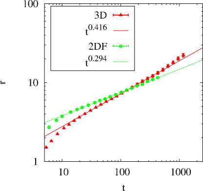
Figure 1: (Color online) This figure shows the power-law scaling of the 2DF ($256\times 256\times 32$ with $\kappa=1$) and 3D ($92^{3}$ with $\kappa=3$) systems at $H=0$ and the deviation from scaling at long times. The error bars were determined by the standard deviation between different runs.

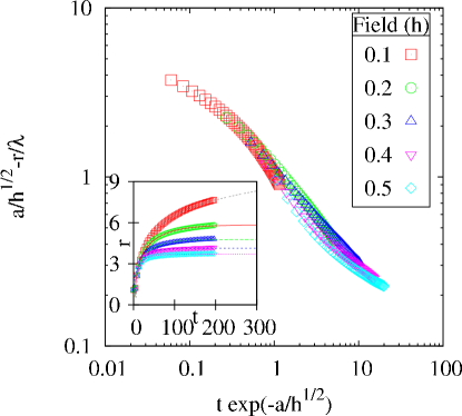
Figure 2: (Color online) Data collapse of the scalings at fields $h=0.1$ to $h=0.5$. The inset compares the inter-vortex spacing to the functional form of Eqn. 13. The values $a=1.626$ and $\lambda=1.810$ were used to produce this collapse. These data are from a 3D simulation at size $92^{3}$ and $\kappa=3$.

V RESULTS

V.1 Three dimensional superconductor in zero external field

For the three dimensional block superconductor, we simulated thirty systems with $96^{3}$ grid cells with physical dimensions $(32r_{core})^{3}$ and $\kappa=3$, starting from a randomized order parameter and allowed to evolve in time. We also simulated five runs of a $128^{3}$ system for longer times in order to observe deflections from the small-$r$ scaling.

The initial state of the order parameter in each cell was chosen by generating a random angle between $0$ and $2\pi$ and a random amplitude between $1$ and $0$, both with a flat distribution. In the case where the superconductor was restricted to a subset of the space (that is, the 2DF system) the amplitude was initialized at zero outside of the thin plate of superconductor. The three components of the vector potential were set to random values between $\pm 1\times 10^{-6}$ in order to break the symmetry of the field and reduce potential artifacts.

We compute the average distance between vortices indirectly by measuring the total volume of vortices in the system and dividing by the cross-sectional area of a vortex, then using that density to obtain the inter-vortex spacing:

$$r=\sqrt{\frac{\pi r_{core}^{2}V}{\int dV(1-|\psi(\vec{r})|^{2})}}$$ (26)

Table 2 summarizes our numerical results and the predictions made here. For comparison, we provide a list (1) of some previous numerical results that have been obtained in simulations of similar systems. The majority of such simulations have been done on 2D and 3D systems with vortex topological defects, but without a gauge field.

For the 3D bulk superconductor, we observe that in the zero-field case after about $t=10$, the behavior is power-law, with an exponent $\phi=0.414\pm 0.01$, in comparison with the prediction from vortex-annihilation dynamics of $\phi=0.429$. In the larger system we observe $t^{0.415}$ scaling, with the behavior deviating from this around $t=600$ (see Fig. 1), possibly due to finite size effects.

¿From our analysis, we also expect a region of logarithmic scaling. At long times $r$ varies logarithmically over a time interval determined by the system size. For all lattice sizes, the behavior between $t=5$ and $t=20$ seems to follow a logarithmic curve which then transitions to the power-law behavior.

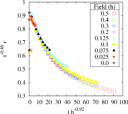
Figure 3: (Color online) Data collapse of the nonzero field scalings according to Eqn. 16. Data are from the same simulation as Fig. 2.

V.2 Two-dimensional superconductor

For the case of a two dimensional sheet with three dimensional fields, we simulated five runs of a system of size $256\times 256\times 32$ grid cells, with $\kappa=1$. The full prediction for that case involves a region of $t^{3/7}$ scaling, followed by a region of $t^{3/10}$ scaling for vortex-annihilation dominated dynamics. As a consequence, for intermediate values of $\kappa$ there is no large scaling range for either regime without waiting long times in the simulation. The smaller the value of $\kappa$, the shorter the time necessary to observe the asymptotic regime and the effect of external three-dimensional fields.

We observe a scaling of $t^{0.294\pm 0.01}$, which is in agreement with the prediction for vortex-annihilation dominated scaling in the large-r limit. The results are shown in Fig. 1.

Eventually, the separation between vortices becomes on the order of the system size and finite size effects appear in the results which puts the final limit on the size of the scaling regime we may observe. This manifests itself as an increase in the fluctuations across different runs and as a sudden sharp upturn in $r$ compared to the power-law prediction, as shown by the data for times $t>600$ in Fig. 1.

V.3 Non-zero field data collapse

The results for a non-zero applied field are in Fig. 2. Here we also plot the best-fit from the predicted form of Eqn. 13 along with each curve. The fits are satisfactory, but break down at short times during the initial quench.

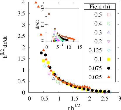
Figure 4: (Color online) Data collapse of the nonzero field time derivatives. $\beta=-1.5$. Data are from the same simulation as Fig. 2.

When we plot the data in terms of the combined variables given by Eqn. 15, we can observe that the time and field-strength variables are not independent. The family of curves we observe will collapse onto a single universal curve given the proper choice of scaling of the variables as we have described in section III.2. The behavior in the absence of a magnetic field also has a crossover - between power-law scaling and logarithmic scaling. The model which generates this collapse does not take into account the power-law scaling and so we expect deviations from the collapse in the case that there is a large regime of power-law scaling ($h\rightarrow 0$). Deviations from the collapse in our simulation are observed at times less than $t=20$ due to the initial quench behavior which is not captured by this model. At sufficiently small fields that the Abrikosov lattice spacing is comparable to the system size we also expect a failure of the collapse at long times - in the zero field case for the $92^{3}$ system this occurs at $t>600$.

In order to capture the power-law scaling behavior, we propose a different form of the data collapse given in Eqn. 16. Plotting the data accordingly we obtain Fig. 3. The scaling exponent $\phi$ was adjusted to give the best visual data collapse, which occurred for $\phi=0.46\pm 0.2$.

The behavior at short times does not collapse, which is consistent with the concept behind this scaling: at short times, the scaling is dominated neither by vortex interactions nor the external magnetic field. Instead, it is the local dynamics of the order parameter which contribute to the inter-vortex spacing. During this time, the measure we have used to determine the inter-vortex spacing cannot be considered meaningful as there are not yet distinct vortex cores.

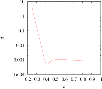
Figure 5: (Color online) Error landscape for the $\dot{r}$ data collapse.

We have also examined the time derivative of the vortex spacing, as this is the basis of the force-law arguments to determine vortex scaling. The behavior of $\dot{r}$ as a function of $r$ at nonzero external fields asymptotes to zero at values of $r$ determined by the external field, i.e. the equilibrium vortex spacings. Rescaling $r$ to map these to the same point results in a new variable $r^{\prime}=\sqrt{h}r$. However, if $\dot{r}$ scales as $r^{\beta}$ in the limit of small $r$, then we must also rescale $\dot{r}$ as follows: $\dot{r}^{\prime}=h^{\beta/2}\dot{r}$. This collapses the data for $\dot{r}$ onto a single curve, as seen in Fig. 4. The value of $\beta$ which best collapses the curves is $\approx-1.5$, which corresponds to a value of the scaling exponent $\phi=0.4$. Unlike the $r$ data collapse, the error landscape of the $\dot{r}$ collapse has a well-defined minimum at finite $\phi$, although there is still a gradual decrease in the error as $\phi$ becomes unphysically large. Figure 5 shows the error in the data collapse measured by $\Delta\equiv\sum_{ijk}{(y_{j}(x_{i})-y_{k}(x_{i}))^{2}}$ where $x_{i}$ is the $i$th rescaled independent variable data point and $y_{j}$ and $y_{k}$ are the interpolated values of the rescaled dependant variable for the $j$th and $k$th field strengths.

The data collapse of Fig. 4 is actually an autonomous counterpart to that of Eqn. 16 as can be readily verified by elimination of $t$.

Now we turn to the small field data, which seems not to obey the data collapse so cleanly. For the $r$ scaling they do not fall onto the data collapse lines nearly as well as the higher fields. However, for the $\dot{r}$ scaling this failure of data collapse is not nearly as pronounced. This may be associated with a bias in the initial spacing introduced by the period immediately after the quench. That is, for the $r$ scaling it may be that rather than measuring time from the simulation start, we must measure it from the end of the quench period when vortex interactions become the dominant effect. However, for the $\dot{r}$ scaling we avoid this by eliminating the time variable and thus removing the problem of an arbitrary initial offset. We will now examine other predictions of the data collapse in order to understand the small field behavior.

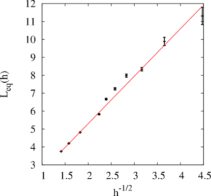
Figure 6: (Color online) Equilibrium vortex spacing at nonzero field. The line is a linear guide. Data are from the same simulation as Fig. 2.

The length scale we observe at long times corresponds to the Abrikosov vortex lattice spacing. Finite system size effects can potentially produce a crossover to the system scale and are more likely to do so for weak field values. The value of the spacing at the longest times accessed by our simulations is plotted versus the field strength in Fig. 6. For sufficiently large fields $h\geq 0.2$ (which corresponds to $h^{-1/2}\leq 2.24$) we see a convergence to the predicted scaling within the time range of our simulation. For small fields we never quite reach the equilibrium scaling. We have however also looked at a $128^{3}$ system at low fields and during the time range of our simulations (up to $t=400$ in this case) we did not observe a significant departure from the $92^{3}$ curves, so the slight deviation from Abrikosov scaling is more likely to be a finite time effect than a finite size effect.

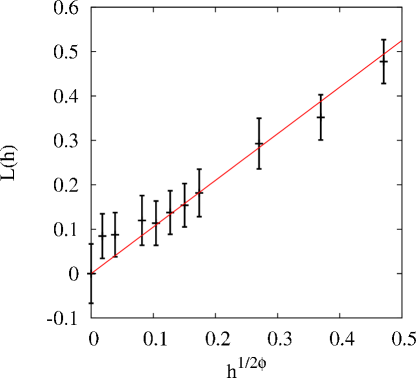
Figure 7: (Color online) Scaling of the vortex spacing in the limit of short times. $\phi=0.46$. The line is a linear guide. Data are from the same simulation as Fig. 2.

We can also make a prediction as to the scaling of $r(h)$ at a fixed small time $t_{1}$. Inserting into the scaling form, we get $r(h,t_{1})={t_{1}}^{\phi}f({t_{1}}^{-\phi}h^{-1/2})$. We wish to Taylor expand $f$ around $t=0$, which we may safely do after writing $\bar{f}\equiv f^{-1/\phi}$, with the result that $r(h,t_{1})={t_{1}}^{-\phi}\bar{f}(t_{1}h^{1/2\phi})\approx C_{1}+C_{2}H^{1/2\phi}t_{1}^{1-\phi}+O({t_{1}}^{2-\phi})$.

We know that $C_{1}=0$ due to the required asymptotic behavior of the scaling function, meaning that we can expect $r(H,t_{1})\propto h^{1/2\phi}$ for fixed small times. The agreement with this prediction is satisfactory, as shown in Fig. 7.

VI CONCLUSIONS

We observed both the case of a three dimensional block of superconductor and a two dimensional sheet via numerical simulation. In the three dimensional block superconductor, we also examined the effect of nonzero external fields, and predicted a scaling form based on the forces between vortices. With this scaling form, we obtained data collapse to a universal curve independent of the value of the external magnetic field. At zero external field, the dynamical critical exponent $\phi$ was found to be in agreement with fluctuation/annihilation arguments rather than the pure vortex-dynamical argument in both the 3D and 2DF systems - that is, in the 3D case we measured $\phi=0.414\pm 0.01$ in comparison with the predicted $3/7$ and in the 2DF case we measured $\phi=0.294\pm 0.01$ in comparison with the predicted $3/10$. We also observed data suggestive of the logarithmic scaling regime at short times between the recovery of the order parameter from the quench and the power-law scaling regime. At long times, we observed deviation from power-law scaling which appears to be a finite size effect. We never observed a regime in which all vortices remaining were of one direction/magnitude of topological charge in the zero-field case. However, with a nonzero field, the majority of vortices in the system are aligned with that field, and so the argument based on vortex dynamics seemed to be more able to predict the scaling form than in the zero-field cases, in which vortex annihilation was always a significant contribution. We have proposed a form for the behavior of the vortex spacing in the presence of external magnetic fields which collapses the data onto a universal curve. We found better collapse when this was applied to the force law as opposed to the actual vortex spacing likely due to the initial time offset in which the order parameter recovers from the quench. This allowed us to explain the behavior at nonzero magnetic field in terms of a crossover from the zero-field scaling to a fixed length scale given by the Abrikosov vortex lattice spacing.