Universal Reduction of Effective Coordination Number
in the Quasi-One-Dimensional Ising Model

Abstract

Critical temperature of quasi-one-dimensional general-spin Ising ferromagnets is investigated by means of the cluster Monte Carlo method performed on infinite-length strips, $L\times\infty$ or $L\times L\times\infty$. We find that in the weak interchain coupling regime the critical temperature as a function of the interchain coupling is well-described by a chain mean-field formula with a reduced effective coordination number, as the quantum Heisenberg antiferromagnets recently reported by Yasuda et al. [Phys. Rev. Lett. 94, 217201 (2005)]. It is also confirmed that the effective coordination number is independent of the spin size. We show that in the weak interchain coupling limit the effective coordination number is, irrespective of the spin size, rigorously given by the quantum critical point of a spin-1/2 transverse-field Ising model.

I Introduction

Effects of interchain coupling in quasi-one-dimensional (Q1D) magnets have been extensively investigated over many years. Theoretically, introduction of an infinitesimal interchain coupling can bring a drastic change to the system; emergence of a thermal phase transition and long-range magnetic order therewith at finite temperatures. In interpreting experimental results on Q1D materials, which mostly exhibit anomalous behavior at finite temperatures, one often has to take the interchain effects into account as well. A standard and established approach for incorporating such a weak interchain interaction is the chain mean-field (CMF) approximation,Scalapino et al. (1975); Schulz (1996) in which a problem in two or three dimensions is reduced to a single-chain model in an effective field by ignoring fluctuations of order parameter between weakly coupled chains. Within the CMF theory, the magnetic susceptibility of a Q1D system is approximated as

$$\chi(T)=\frac{\chi_{\text{1d}}(T)}{1-zJ^{\prime}\chi_{\text{1d}}(T)},$$ (1)

where $\chi_{\text{1d}}(T)$ is the susceptibility of a genuinely one-dimensional chain, $z$ the coordination number, i.e., the number of nearest neighbor sites in directions perpendicular to the chain, and $J^{\prime}$ is the interchain coupling constant in these directions. Since $\chi_{\text{1d}}(T)$ may not have any singularity at finite temperatures, the critical temperature $T_{\text{c}}$ of the Q1D system is given as the locus of the simple pole in the right-hand side (rhs) of Eq. (1). That is,

$$z=\frac{1}{J^{\prime}\chi_{\text{1d}}(T_{\text{c}})}$$ (2)

is the equation which determines the Q1D critical temperature. It has been confirmed that for various Q1D (and also Q2D) materials the solution of the CMF self-consistent equation (2) reproduces a qualitatively acceptable $J^{\prime}$-dependence of the critical temperature in the weak interchain coupling regime.

Recently, Yasuda et al.Yasuda et al. (2005) carefully reexamined the Néel temperature of the quantum Heisenberg antiferromagnets on a anisotropic cubic lattice, and found that Eq. (2) does not hold even in the weak interchain coupling limit. In Ref. Yasuda et al., 2005, the rhs of Eq. (2) for various $J^{\prime}$’s is evaluated accurately by the extensive quantum Monte Carlo simulation using the continuous-imaginary-time loop algorithm, and it is concluded that for $J^{\prime}\rightarrow 0$ it converges not to 4 but to 2.78 for the Heisenberg antiferromagnets on the Q1D cubic lattice. This discrepancy with the CMF theory is interpreted as a reduction of the effective coordination number

$$\zeta(J^{\prime})\equiv\frac{1}{J^{\prime}\chi_{\text{1d}}(T_{\text{c}}(J^{\prime}))}$$ (3)

from that of the original lattice, $z$. Furthermore, the numerical data presented in Ref. Yasuda et al., 2005 clearly demonstrate that the renormalized coordination number is “universal,” i.e., independent of the spin size $S$ (including the classical limit $S=\infty$). Although there have been several attemptsIrkhin and Katanin (1997, 1998); Irkhin et al. (1999); Irkhin and Katanin (2000); Bocquet (2002); Hastings and Mudry (2006); Praz et al. ; Yao and Sandvik to develop theories beyond the CMF for specific models so far, our understanding of $S$-independent renormalization of the effective coordination number is, fairly speaking, not yet satisfactory.

Another interesting question is whether and how such a renormalization of the effective coordination number is observed for other models than the Heisenberg antiferromagnets. Among many theoretical spin models, a linear array of $S=1/2$ Ising chains, which forms an anisotropic square lattice, provides a valuable example, since the exact critical temperature is known for any ratio of $J^{\prime}$ to the intrachain coupling $J$. Indeed it was pointed out more than three decades agoScalapino et al. (1975) that the CMF result for the critical temperature

$$T_{\text{c}}\simeq\frac{J}{2\ln(J/J^{\prime})-2\ln\ln(J/J^{\prime})}$$ (4)

for $J^{\prime}/J\ll 1$ is not compatible with the exact asymptotic behavior

$$T_{\text{c}}\simeq\frac{J}{2\ln(2J/J^{\prime})-2\ln\ln(2J/J^{\prime})}.$$ (5)

Here and hereafter we put the Boltzmann constant to unity. The former asymptotic expression is obtained from Eq. (2) with $z=2$, combined with the exact susceptibility of an $S=1/2$ single Ising chain

$$\chi_{\text{1d}}^{1/2}(T)=\frac{1}{4T}e^{J/2T},$$ (6)

whereas the latter is obtained by expanding Onsager’s exact solution for the anisotropic Ising modelOnsager (1944)

$$\sinh\frac{J}{2T_{\text{c}}}\sinh\frac{J^{\prime}}{2T_{\text{c}}}=1$$ (7)

for small $J^{\prime}/J$. [Note that here the absolute spin length is not 1 but 1/2. See the definition of our Hamiltonian (8) below.] Interestingly, if the effective coordination number [Eq. (3)] is evaluated for this case by using the exact critical temperature and the exact one-dimensional susceptibility, Eqs. (6) and (7) respectively, one immediately finds that it converges to unity, instead of 2, in the $J^{\prime}/J=0$ limit.Praz et al. This example thus clearly demonstrates the breakdown of the CMF approach for Q1D magnets, to which we will address ourselves in the present work.

In the present paper, we report our detailed analysis on the Q1D general-spin Ising models, and discuss the origin of the $S$-independent renormalization in the effective coordination number in the weak interchain coupling regime. The organization of the paper is as follows: In Sec. II, we define our models and summarize some basic properties in the genuinely one-dimensional case. In Sec. III, we describe our Monte Carlo method and the detail of finite-size scaling analysis. The main results of our Monte Carlo simulation are presented in Sec. IV, where we unambiguously show that the critical temperature is described quite well by a CMF formula with a reduced effective coordination number. The effective coordination number is found independent of $S$ in the weak interchain coupling limit, but does depend on the dimensionality of the lattice as well as on the fine structure of the lattice in directions perpendicular to the chains. In Sec. V, we discuss the origin of the “universality” (or “nonuniversality”) by considering a mapping to a quantum Ising model in the weak interchain coupling limit. We show that the original spin-$S$ Ising model is mapped onto the spin-$1/2$ transverse-field Ising model, irrespective of the spin size, and furthermore the effective coordination number in this limit is rigorously independent of $S$ and given by the quantum critical point of the mapped $S=1/2$ transverse-field Ising model. Our results and conclusions are summarized in Sec. VI.

II Quasi-one-dimensional Ising Model

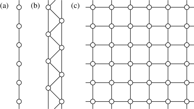
Figure 1: Lattice structures in the transverse directions perpendicular to the chains: (a) square lattice (SQ), (b) square lattice with anisotropic next-nearest-neighbor interaction (SQ+ANNNI), and (c) simple cubic lattice (SC). All the bonds shown in the figure have the exchange coupling of the same strength, $J^{\prime}$.

We consider the following classical spin-$S$ Ising model:

$${\cal H}=-J\sum_{i,\bm{r}}S_{i,\bm{r}}^{z}S_{i+1,\bm{r}}^{z}-J^{\prime}\sum_{i,\bm{r},\bm{\delta}}S_{i,\bm{r}}^{z}S_{i,\bm{r}+\bm{\delta}}^{z},$$ (8)

where $i$ and $\bm{r}$ are the position of lattice sites along chains and perpendicular directions, respectively, $\bm{\delta}$ is summed over the $z/2$ nearest-neighbor vectors in the transverse directions, and $S_{i,\bm{r}}^{z}$ $(=S,S-1,\ldots,-S)$ is the spin variable at site $(i,\bm{r})$. Both of the longitudinal and transverse coupling constants, $J$ and $J^{\prime}$, are assumed to be ferromagnetic ($J\geq J^{\prime}>0$).

In the present study, three different Q1D lattices are considered: square lattice (SQ), square lattice with anisotropic next-nearest-neighbor interaction (SQ+ANNNI), and simple cubic lattice (SC). In Fig. 1, the lattice structure in a slice perpendicular to the chains are drawn. The former two (SQ and SQ+ANNNI) are two-dimensional lattices, while the last one (SC) is three dimensions. On the other hand, the latter two shares the same coordination number, $z=4$, which is larger than that of the first lattice ($z=2$). By considering these three lattices, one can evaluate separately the effects of dimensionality from the coordination number.

The linear dimension of the lattice in the directions perpendicular to the chains is specified by $L$. We assume periodic boundary conditions in these directions. For the SQ and SQ+ANNNI lattices, the number of spins in each slice, denoted by $N_{\text{s}}$ hereafter, is equal to $L$, while it is $L^{2}$ for the SC lattice. In the chain direction, on the other hand, the system size is assumed to be infinite as explained in the next section.

Before starting a detailed discussion about the critical temperature of the Q1D system, let us briefly review thermal properties of a genuinely one-dimensional single chain, i.e., Eq. (8) with $J^{\prime}=0$, since its susceptibility $\chi_{\text{1d}}(T)$ appears as a key quantity in the CMF approximation, and thus is expected to dominate asymptotic behavior of the critical temperature $T_{\text{c}}(J^{\prime})$ for $J^{\prime}\ll J$.

The partition function of a periodic spin-$S$ Ising chain of length $M$ is represented asKramers and Wannier (1941)

$$Z_{\text{1d}}=\text{tr}\,\bm{T}^{M}.$$ (9)

Here the transfer matrix $\bm{T}$ is a $(2S+1)\times(2S+1)$ real symmetric matrix with matrix elements

$$\bm{T}_{ij}=e^{J(S+1-i)(S+1-j)/T}.$$ (10)

The matrix $\bm{T}$ is diagonalized as

$$\bm{T}=\bm{U}\bm{D}\bm{U}^{-1}$$ (11)

by a diagonal matrix of eigenvalues, $\bm{D}_{ij}=\lambda_{i}\delta_{i,j}$, and a matrix of the corresponding right (column) eigenvectors, $\bm{U}=(u_{1},u_{2},\ldots,u_{2S+1})$ with $\bm{T}u_{i}=\lambda_{i}u_{i}$. We assume all the eigenvectors are normalized, i.e., $\bm{U}^{-1}=\,^{t}\bm{U}$. Without loss of generality we further assume $\lambda_{1}$ and $\lambda_{2}$ denote the largest and the second largest eigenvalues, respectively.

At finite temperatures, the transfer matrix $\bm{T}$ is positive definite and its largest eigenvalue $\lambda_{1}$ is nondegenerate. Thus the partition function (9) is evaluated as $(\lambda_{1})^{M}$ in the thermodynamic limit. Similarly, the thermal average of correlation function between the spins at site 0 and $r$ is calculated in terms of the transfer matrix as

$$\begin{split}\langle S^{z}_{0}S^{z}_{r}\rangle&=\frac{1}{Z}\text{tr}\,\bm{S}\bm{T}^{r}\bm{S}\bm{T}^{M-r}\\ &=\frac{1}{Z}\text{tr}\,(\bm{U}^{-1}\bm{S}\bm{U})\bm{D}^{r}(\bm{U}^{-1}\bm{S}\bm{U})\bm{D}^{M-r}\\ &\!\!\!\!\underset{M\rightarrow\infty}{\longrightarrow}\lambda_{1}^{-r}\text{tr}\,(\bm{U}^{-1}\bm{S}\bm{U})\bm{D}^{r}(\bm{U}^{-1}\bm{S}\bm{U})\\ &=\sum_{i=2}^{2S+1}|^{t}u_{1}\bm{S}u_{i}|^{2}\Big{(}\frac{\lambda_{i}}{\lambda_{1}}\Big{)}^{r},\end{split}$$ (12)

where we introduce $\bm{S}_{ij}=(S+1-i)\delta_{i,j}$. In the last expression, we explicitly dropped $i=1$ in the summation, since $(^{t}u_{1}\bm{S}u_{1})$ constantly vanishes due to the spin inversion symmetry in the Hamiltonian (8). The susceptibility is then obtained by summing up the correlation function over the whole lattice

$$\begin{split}\chi_{\text{1d}}(T)&=\frac{1}{T}\sum_{r=-\infty}^{\infty}\langle S^{z}_{0}S^{z}_{r}\rangle=\frac{1}{T}\sum_{i=2}^{2S+1}|^{t}u_{1}\bm{S}u_{i}|^{2}\frac{\lambda_{1}+\lambda_{i}}{\lambda_{1}-\lambda_{i}}.\end{split}$$ (13)

For $S=1/2$, 1, and $3/2$, all the eigenvalues and the eigenvectors of the transfer matrix can be obtained explicitly in a closed form, and so is the susceptibility.Suzuki et al. (1967) For larger $S$, it is not able to solve the eigenvalue problem analytically, but one can still diagonalize $\bm{T}$ numerically very easily.

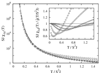
Figure 2: Scaling plot of susceptibility of a single chain with $S=1/2$ (solid line), 1 (diamonds), 3/2 (upward triangles), 2 (downward triangles), 4 (circles), and 8 (squares). In the inset, corrections to the low-temperature asymptotic form [Eq. (24)] are presented.

At very low temperatures, $T\ll J$, the largest two eigenvalues $\lambda_{1}$ and $\lambda_{2}$ nearly degenerate with each other, which reflects two degenerating fully polarized ground states, $(S,S,\ldots,S)$ and its spin-inverted counterpart, with energy $-S^{2}JM$. The corresponding eigenvectors are symmetric or antisymmetric, respectively, under the spin inversion, and their elements are given as follows:

$$u_{1,1} =u_{1,2S+1}=\frac{1}{\sqrt{2}}+O(e^{-J/T}),$$ (14)

$$u_{1,i} =O(e^{-J/T})\ \ \text{for $i=2,\ldots,2S$,}$$ (15)

$$u_{2,1} =-u_{1,2S+1}=\frac{1}{\sqrt{2}}+O(e^{-J/T}),$$ (16)

$$u_{2,i} =O(e^{-J/T})\ \ \text{for $i=2,\ldots,2S$}.$$ (17)

The absolute value of the subdominant eigenvalues is exponentially small in comparison with the largest two. The correlation function and the susceptibility at low temperatures are thus written as

$$\langle S^{z}_{0}S^{z}_{r}\rangle \simeq S^{2}\Big{(}\frac{\lambda_{2}}{\lambda_{1}}\Big{)}^{r}\ \ \text{and}$$ (18)

$$\chi_{\text{1d}}(T) \simeq\frac{S^{2}}{T}\frac{\lambda_{1}+\lambda_{2}}{\lambda_{1}-\lambda_{2}},$$ (19)

respectively. By defining the correlation length $\xi_{\text{1d}}(T)$ as $\xi_{\text{1d}}^{-1}(T)=-\log(\lambda_{2}/\lambda_{1})$, we obtain

$$\chi_{\text{1d}}(T) \simeq\frac{S^{2}}{T}\frac{1+e^{-1/\xi_{\text{1d}}(T)}}{1-e^{-1/\xi_{\text{1d}}(T)}}\simeq\frac{2S^{2}}{T}\xi_{\text{1d}}(T)$$ (20)

for general spin $S$. For $S=1$ and 3/2, the low-temperature susceptibility is explicitly given bySuzuki et al. (1967)

$$\chi_{\text{1d}}^{1}(T) \simeq\frac{1}{2T}e^{2J/T}\ \ \text{and}$$ (21)

$$\chi_{\text{1d}}^{3/2}(T) \simeq\frac{3}{4T}e^{9J/2T},$$ (22)

respectively. [The exact expression for $S=1/2$ is already presented in Eq. (6).] For larger $S$, analytic expressions are not known, but low-temperature asymptotic forms for the correlation length and the susceptibility are conjectured as follows:

$$\begin{split}\xi_{\text{1d}}^{S}(T)&\simeq-\Big{[}2S\log\Big{(}\tanh\frac{S^{2}J}{T}\Big{)}\Big{]}^{-1}\\ &\simeq\frac{1}{4S}e^{2S^{2}J/T}=\frac{1}{S}\tilde{f}(T/S^{2}J)\end{split}$$ (23)

and

$$\chi_{\text{1d}}^{S}(T) \simeq\frac{S}{2T}e^{2S^{2}J/T}=\frac{1}{SJ}\tilde{g}(T/S^{2}J),$$ (24)

where $\tilde{f}(x)=e^{2/x}/4$ and $\tilde{g}(x)=e^{2/x}/2x$ are scaling functions. These expressions are confirmed explicitly, e.g., Eqs. (6), (21), and (22), for $S\leq 3/2$. We emphasize that these scaling forms are not very trivial. Indeed, a naive dimensional analysis yields $\xi_{\text{1d}}^{S}(T)\simeq\tilde{f}(T/S^{2}J)$ and $\chi_{\text{1d}}^{S}(T)\simeq J^{-1}\tilde{g}(T/S^{2}J)$ with some scaling functions $\tilde{f}(x)$ and $\tilde{g}(x)$, which differs from the correct scaling forms presented above by a factor $1/S$. In Fig. 2, we present a scaling plot of the numerically exact data for the susceptibility, given by Eq. (13), for $S=1/2,1,\ldots,8$, which confirms the asymptotic scaling formula (24).

III Numerical Method

III.1 Cluster Monte Carlo on infinite-length strip

For the $S=1/2$ SQ lattice, the critical temperature is solved exactly for any combination of $J^{\prime}$ and $/J$ as we have already seen in Sec. I. However, no exact solutions are available for $S\geq 1$. For the other lattices (SQ+ANNNI and SC) there are no solutions even for $S=1/2$.

In the present study we employ the Monte Carlo method combined with the finite-size scaling analysis for evaluating unbiased critical temperatures of the Q1D Ising models. Since the present model has only the ferromagnetic couplings and has no frustration, the Swendsen-Wang cluster algorithm,Swendsen and Wang (1987) or the Wolff cluster algorithm,Wolff (1989) is one of the best algorithms. To optimize further for the Q1D general-spin Ising models, we extend the cluster Monte Carlo algorithm in the following two points.

The first optimization is for strong anisotropy. Since our model is strongly spatially anisotropic, one has to fine-tune the aspect ratio of the lattice to simulate an effectively large system with a reasonable cost.Yasuda et al. (2005); Matsumoto et al. (2001) In the present study, instead of anisotropic finite lattices, we simulate infinite length strips $N_{\text{s}}\times\infty$ directly, following the infinite-lattice algorithm proposed by Evertz and von der Linden.Evertz and von der Linden (2001) In the original proposal of the infinite-lattice cluster algorithm, the lattice is assumed to be infinite in all the spatial directions and only one cluster including the origin is build at each Monte Carlo step. In our simulation, however, the lattice is infinite only in one direction, the chain direction, which has a stronger coupling than the transverse directions, and we build up completely all clusters including the $N_{\text{s}}$ sites on the slice in the center of the lattice at each Monte Carlo step. This modification avoids the divergence of cluster size and enables us the simulation at and below the critical temperature of the bulk and thus the finite-size scaling for accurate estimation the critical temperature.

Another modification to the original cluster algorithm is the extension for general spin $S>1/2$.Todo and Kato (2000, 2001) To this end, first we decompose a spin into $2S$ subspins, that is, we simulate the following $S=1/2$ model

$$\begin{split}{\cal H}_{\text{subspin}}=&-J\sum_{i,\bm{r}}\sum_{\alpha,\alpha^{\prime}=1}^{2S}\tilde{S}_{i,\bm{r},\alpha}^{z}\tilde{S}_{i+1,\bm{r},\alpha^{\prime}}^{z}\\ &-J^{\prime}\sum_{i,\bm{r},\bm{\delta}}\sum_{\alpha,\alpha^{\prime}=1}^{2S}\tilde{S}_{i,\bm{r},\alpha}^{z}\tilde{S}_{i,\bm{r}+\bm{\delta},\alpha^{\prime}}^{z},\end{split}$$ (25)

instead of the original spin-$S$ model. Here $\tilde{S}_{i,\bm{r},\alpha}=\pm 1/2$ is the $\alpha$th subspin at site $(i,\bm{r})$. The volume of the phase space of the mapped system (25) is enlarged than the original one [from $(2S+1)^{N}$ to $2^{2SN}$, where $N$ is the number of original spins]. We need an extra procedure which symmetrize each spin to recover the original phase spaceTodo and Kato (2000, 2001) as described below.

A Monte Carlo step is as follows: (i) set $i\mapsto 0$; (ii) every possible subspin pair, $\tilde{S}_{i,\bm{r},\alpha}$ and $\tilde{S}_{i,\bm{r+\delta},\alpha^{\prime}}$, in the $i$th slice is connected with probability $(1-e^{-2J^{\prime}/T})$ if $\tilde{S}_{i,\bm{r},\alpha}=\tilde{S}_{i,\bm{r+\delta},\alpha^{\prime}}$, or left disconnected otherwise; (iii) for each group of subspins $(i,\bm{r})$, the subspins are partitioned into two according to their spin direction, a random permutation is generated for each part, and the subspins belonging to the same permutation cycle are connected with probability one; (iv) every possible subspin pair, $\tilde{S}_{i,\bm{r},\alpha}$ and $\tilde{S}_{i+1,\bm{r},\alpha^{\prime}}$, on the neighboring slices, $i$ and $i+1$, is connected with probability $(1-e^{-2J/T})$ if $\tilde{S}_{i,\bm{r},\alpha}=\tilde{S}_{i+1,\bm{r},\alpha^{\prime}}$, or left disconnected otherwise; (v) increase $i$ by 1 and repeat (ii)–(iv) until no clusters in the current slice include any subspins on the central slice at $i=0$; (vi) repeat (ii)–(v) in the opposite chain direction, $i=-1,-2,\ldots$; (vii) generate a new spin configuration by flipping all subspins on each cluster including the subspins on the central slice randomly with probability $1/2$, and discard all the clusters.

The present method satisfies detailed balance conditions and ergodicity for any finite region including the central slice. Typically, we spend $1.0\times 10^{6}$ Monte Carlo steps for measurement after discarding $3.3\times 10^{4}$ steps for thermalization for each parameter set $(J^{\prime}/J,T/J,L)$.

III.2 Susceptibility and correlation length

Correlation functions $\langle S^{z}_{i,\bm{r}}S^{z}_{i^{\prime},\bm{r}^{\prime}}\rangle$ can be measured efficiently in terms of a neat technique, so called improved estimator,Wolff (1989) i.e.,

$$\langle S^{z}_{i,\bm{r}}S^{z}_{i^{\prime},\bm{r}^{\prime}}\rangle=\frac{1}{4}\sum_{\alpha,\alpha^{\prime}}\langle C(i,\bm{r},\alpha;i^{\prime},\bm{r}^{\prime},\alpha^{\prime})\rangle_{\text{MC}},$$ (26)

where $\langle\cdots\rangle_{\text{MC}}$ denotes a Monte Carlo average and $C(i,\bm{r},\alpha;i^{\prime},\bm{r}^{\prime},\alpha^{\prime})$ takes 1 if the subspins at $(i,\bm{r},\alpha)$ and $(i^{\prime},\bm{r}^{\prime},\alpha^{\prime})$ belong to the same cluster and takes 0 otherwise at each Monte Carlo step. We can further rewrite Eq. (26) by introducing a function $C_{\ell}(i,\bm{r},\alpha)$, which takes 1 if the subspin $\tilde{S}^{z}_{i,\bm{r},\alpha}$ is on the $\ell$th cluster and takes 0 otherwise, as

$$\langle S^{z}_{i,\bm{r}}S^{z}_{i^{\prime},\bm{r}^{\prime}}\rangle=\frac{1}{4}\sum_{\alpha,\alpha^{\prime}}\Big{\langle}\sum_{\ell}C_{\ell}(i,\bm{r},\alpha)C_{\ell}(i^{\prime},\bm{r}^{\prime},\alpha^{\prime})\Big{\rangle}_{\text{MC}}.$$ (27)

Here one must recall that in the present algorithm clusters will be built only for a part of the lattice, and there is no way to judge whether two subspins belong to the same cluster when neither is on the built clusters. Therefore the above improved estimator for the correlation function is valid only if at least one of $(i,\bm{r},\alpha)$ and $(i^{\prime},\bm{r}^{\prime},\alpha^{\prime})$ is guaranteed to belong always to built clusters. Since only the subspins on the central slice satisfies this condition, $i$ or $i^{\prime}$ must be zero in Eqs. (26) and (27).

The magnetic susceptibility $\chi$ is obtained by integrating the correlation function over the whole lattice. Fixing $i=0$ in Eq. (26) and taking a sum over all the other indices, we obtain the following expression for the susceptibility:

$$\begin{split}\chi&=\frac{1}{TN_{\text{s}}}\sum_{i=-\infty}^{\infty}\sum_{\bm{r},\bm{r}^{\prime}}\langle S^{z}_{0,\bm{r}}S^{z}_{i,\bm{r}^{\prime}}\rangle\\ &=\frac{1}{4TN_{\text{s}}}\sum_{i=-\infty}^{\infty}\sum_{\bm{r},\bm{r}^{\prime},\alpha,\alpha^{\prime}}\Big{\langle}\sum_{\ell}C_{\ell}(0,\bm{r},\alpha)C_{\ell}(i,\bm{r}^{\prime},\alpha^{\prime})\Big{\rangle}_{\text{MC}}\\ &=\frac{1}{4TN_{\text{s}}}\Big{\langle}\sum_{\ell}n_{\ell}^{(0)}n_{\ell}\Big{\rangle}_{\text{MC}},\end{split}$$ (28)

where $n_{\ell}^{(0)}\equiv\sum_{\bm{r},\alpha}C_{\ell}(0,\bm{r},\alpha)$ denotes the number of subspins on the central slice in the $\ell$th cluster, and $n_{\ell}\equiv\sum_{i,\bm{r},\alpha}C_{\ell}(i,\bm{r},\alpha)$ is the number of subspins in the $\ell$th cluster.

The correlation length along the strip is estimated as

$$\xi_{k,k^{\prime}}=\Big{(}\frac{X_{k}}{X_{k^{\prime}}}\Big{)}^{1/(k-k^{\prime})},$$ (29)

with nonnegative integers, $k\neq k^{\prime}$, and the moments of the correlation function

$$\begin{split}X_{k}&=\frac{1}{k!N_{\text{s}}}\sum_{i=-\infty}^{\infty}\sum_{\bm{r},\bm{r}^{\prime}}|i|^{k}\langle S^{z}_{0,\bm{r}}S^{z}_{i,\bm{r}^{\prime}}\rangle\\ &=\frac{1}{4k!N_{\text{s}}}\Big{\langle}\sum_{\ell}n_{\ell}^{(0)}m_{\ell}^{k}\Big{\rangle}_{\text{MC}},\end{split}$$ (30)

where $m_{\ell}^{k}\equiv\sum_{i,\bm{r},\alpha}|i|^{k}C_{\ell}(i,\bm{r},\alpha)$. Note that the moment $X_{k}$ converges for any integer $k\geq 0$, since the correlation function decays exponentially on a finite-width strip even below the critical temperature. In the following analysis we use the simplest estimator, $\xi_{1,0}=X_{1}/X_{0}$, since its statistical error is the smallest among all the combinations $(k,k^{\prime})$ we examined.

III.3 Finite-size scaling analysis

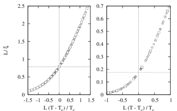
Figure 3: Scaling plots of the correlation length for the $S=1/2$ SQ lattices with $J^{\prime}/J=1$ (left) and $J^{\prime}/J=0.1$ (right). System sizes are $L=22,24,\ldots,30$ and $L=14,16,\ldots,24$, respectively. The error bar of each point is much smaller than the symbol size. The critical temperature and the critical amplitude are estimated as $T_{\text{c}}/S^{2}J=2.2695(3)$ and $L/\xi|_{T=T_{\text{c}}}=0.789(3)$ for $J^{\prime}/J=1$, and $T_{\text{c}}/S^{2}J=0.9058(2)$ and $L/\xi|_{T=T_{\text{c}}}=0.176(1)$ for $J^{\prime}/J=0.1$, respectively

Near the critical point $T=T_{\text{c}}$ the correlation length and the susceptibility of a finite system obey the following finite-size scaling formulas:

$$L/\xi(L,T) =\tilde{\xi}(L^{1/\nu}(T-T_{\text{c}})/T_{\text{c}})\ \ \text{and}$$ (31)

$$L^{-\gamma/\nu}\chi(L,T) =\tilde{\chi}(L^{1/\nu}(T-T_{\text{c}})/T_{\text{c}}),$$ (32)

where $\nu$ and $\gamma$ are the critical exponents of the correlation length and of the susceptibility respectively, and $\tilde{\xi}(x)$ and $\tilde{\chi}(x)$ are scaling functions. In the following analysis we assume the critical exponents of the Ising universality, i.e., $\nu=1$ and $\gamma/\nu=7/4$ for SQ and SQ+ANNNI, and $\nu=0.6289$ and $\gamma/\nu=1.9828$ for SC.Ferrenberg and Landau (1991) The critical temperature is then determined as the point where all the data points collapse best on a single curve.

As a test of the numerical method explained in this section, we perform a Monte Carlo simulation and a finite-size scaling analysis for $S=1/2$ SQ lattices with $J^{\prime}/J=1$ and 0.1. In Fig. 3, we presents scaling plots of the correlation length. All the data points collapse excellently on a single curve in both cases. The critical temperature is estimated as $T_{\text{c}}/S^{2}J=2.2695(3)$ and 0.9058(2) for $J^{\prime}/J=1$ and 0.1, respectively, which coincide with the exact values $T_{\text{c}}/S^{2}J\approx 2.26919$ and $0.90588$.

Here we comment that the present lattice geometry $L\times\infty$ is the same as the one used for the phenomenological renormalization calculation of the transfer matrix. As a result, not only the critical exponents but also the critical amplitude of the correlation length along the strip is given analytically in the isotropic case ($J^{\prime}=J$) due to the conformal invariance of the model at the critical point.Cardy (1984) We confirm that the critical amplitude $L/\xi|_{T=T_{\text{c}}}=0.789(3)$ for $J^{\prime}/J=1$ (Fig. 3) agrees with $\pi/4\approx 0.785$, the prediction from the conformal field theory. In anisotropic cases $J^{\prime}\neq J$, a nonuniversal prefactor, which represents effective aspect ratio, is introduced and thus the overall critical amplitude becomes nonuniversal. However, this gives us a chance to estimate the effective aspect ratio at the critical point directly. For example, we can estimate the effective aspect ratio immediately as $0.789/0.176\approx 4.48$ for $J^{\prime}/J=0.1$. This method works also for the three-dimensional case (but does not for the SQ+ANNNI lattice due to the anisotropy intrinsic to the lattice). On the other hand, it is practically a hard task if one works in the standard square or cubic geometry, $L\times L^{\prime}$ or $L\times L^{\prime}\times L^{\prime\prime}$, for Monte Carlo simulations. This is another advantage of the present Monte Carlo method for analyzing spatial anisotropy precisely, though we will not utilize this quantity in the remainder of this paper.

IV Results of Monte Carlo Simulation

By using the Monte Carlo method and the finite-size-scaling technique explained in the last section, we estimate the critical temperature of the SQ, SQ+ANNNI, and SC lattices very carefully for $S=1/2$, 1, and $3/2$ and $J^{\prime}/J=0.001,0.002,0.005,\ldots,1$. The error bar of the estimates is typically less than 0.01%. Such a high accuracy for the critical temperature is essential for a reliable estimation of the effective coordination number especially for small $J^{\prime}/J$, where any small error in $T_{\text{c}}$ is amplified vastly due to the exponential growth of the single-chain susceptibility at low temperatures. The results are summarized in Tables 3, 3, and 3, together with the maximum system size for each value of $J^{\prime}/J$.

The present estimates of the critical temperature for the $S=1$ and 3/2 isotropic SQ lattices ($J^{\prime}/J=1$) can be compared with the previous high-temperature series expansion study,Butera et al. (2003) $T_{\text{c}}/S^{2}J=1.69356(1)$ and $1.46144(1)$, respectively. The result for the $S=1/2$ isotropic SC lattice also agrees with the previous Monte Carlo study,Ferrenberg and Landau (1991) $T_{\text{c}}/S^{2}J=4.511424(53)$ within the error bar.

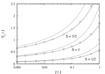
Figure 4: $J^{\prime}$-dependence of the critical temperature for the SQ lattice by the CMF approximation (dashed lines) compared with the exact [$S=1/2$ (squares)] and the Monte Carlo [$S=1$ (diamonds) and 3/2 (circles)] results. Solid lines denote the CMF results with a renormalized coordination number $\zeta=1$ (see the text for details). The error bar of the data for $S=1$ and 3/2 is much smaller than the symbol size.

For all the lattices and all the spin sizes we examined, the critical temperature, normalized by $J$, becomes lower with decreasing $J^{\prime}/J$, as expected. The decrease is found extremely slow. Even at $J^{\prime}/J=0.001$ the critical temperature is as high as 10%–20% of the isotropic case. This slow decrease is explained, within the CMF theory, as a reflection of exponential divergence of the single-chain susceptibility [Eq. (24)].

In Fig. 4, we plot the critical temperature of the SQ lattice as a function of $J^{\prime}/J$ together with the estimates by the CMF approximation, i.e., the numerical solutions of Eq. (2). One sees that the CMF theory constantly overestimates the critical temperature. This tendency is naturally understood as a systematic error subsistent in the approximation, introduced by ignoring fluctuations of order parameter between chains. Although the deviation of the CMF results from the correct $T_{\text{c}}(J^{\prime})$ becomes smaller with decreasing $J^{\prime}/J$, its convergence is logarithmically slow for all the spin sizes, as demonstrated for $S=1/2$ in Sec. I. Similar $J^{\prime}$-dependence of the critical temperature is observed for the other lattices.

In Sec. I, we see that the effective coordination number for the $S=1/2$ SQ lattice converges to unity instead of 2, which indicates that the critical temperature in the weak interchain coupling regime is well-described by a CMF approximation with the renormalized coordination number, $\zeta=1$. In Fig. 4, we also plot the results of the CMF approximation with $\zeta=1$ by solid lines, which amazingly agrees with the true critical temperature in a very wide range of $J^{\prime}/J$; even at $J^{\prime}/J=1$, deviation from the correct value is only 3%, 2%, and 4% for $S=1/2$, 1, and 3/2, respectively, which is much smaller than those of the conventional CMF theory, 55%, 43%, and 39%. For $J^{\prime}/J\lesssim 0.1$, deviation cannot be recognized anymore by the present scale of the vertical axis in Fig. 4.

Table 1: Critical temperature and effective coordination number of the SQ lattice for $S=1/2$, 1, and 3/2. The critical temperature for $S=1/2$ is obtained from Eq. (7). The effective coordination number for $S=1$ and 3/2 in the $J^{\prime}/J=0$ limit, presented in the bottom row, is estimated by taking an average for $J^{\prime}/J=0.001$, 0.002 and 0.005.

		$S=1/2$		$S=1$		$S=3/2$
$J^{\prime}/J$	$L_{\text{max}}$	$T_{\text{c}}/S^{2}J$	$\zeta$	$T_{\text{c}}/S^{2}J$	$\zeta$	$T_{\text{c}}/S^{2}J$	$\zeta$
1	72	2.26919	0.939927	1.6934(2)	1.0492(2)	1.4611(1)	1.0907(2)
0.5	48	1.64102	0.970162	1.2352(1)	1.0430(2)	1.0686(1)	1.0731(3)
0.2	44	1.14156	0.989893	0.88657(5)	1.0230(2)	0.77513(5)	1.0393(2)
0.1	40	0.905883	0.995958	0.72490(7)	1.0111(4)	0.64059(6)	1.0191(4)
0.05	36	0.741313	0.998486	0.61061(3)	1.0045(2)	0.54589(3)	1.0082(3)
0.02	36	0.590681	0.999618	0.50250(2)	1.0010(2)	0.45587(2)	1.0021(2)
0.01	36	0.508926	0.999871	0.44146(2)	1.0002(3)	0.40448(2)	1.0004(3)
0.005	32	0.445462	0.999958	0.39256(2)	0.9998(3)	0.36285(2)	0.9999(4)
0.002	32	0.380981	0.999991	0.34134(1)	0.9999(2)	0.31863(2)	0.9997(5)
0.001	32	0.342657	0.999997	0.31008(2)	0.9997(5)	0.29131(2)	1.0000(6)
			1		0.99989(6)		0.99986(9)

Table 2: Critical temperature and effective coordination number of the SQ+ANNNI lattice for $S=1/2$, 1, and 3/2. The effective coordination number in the $J^{\prime}/J=0$ limit, presented in the bottom row, is estimated by taking an average for $J^{\prime}/J=0.001$, 0.002 and 0.005.

		$S=1/2$		$S=1$		$S=3/2$
$J^{\prime}/J$	$L_{\text{max}}$	$T_{\text{c}}/S^{2}J$	$\zeta$	$T_{\text{c}}/S^{2}J$	$\zeta$	$T_{\text{c}}/S^{2}J$	$\zeta$
1	72	3.8487(9)	2.2889(8)	2.8064(4)	2.5325(6)	2.4032(2)	2.6157(3)
0.5	48	2.5799(3)	2.3766(5)	1.8790(3)	2.5656(8)	1.6084(2)	2.6223(6)
0.2	44	1.6451(1)	2.4388(3)	1.2240(1)	2.5495(5)	1.0548(1)	2.5947(6)
0.1	40	1.2378(1)	2.4600(5)	0.9478(2)	2.522(2)	0.8244(1)	2.550(1)
0.05	36	0.97023(6)	2.4698(5)	0.76744(5)	2.4990(6)	0.67517(7)	2.513(1)
0.02	36	0.73958(5)	2.4747(6)	0.60904(4)	2.4831(7)	0.54444(4)	2.4889(8)
0.01	36	0.62076(3)	2.4757(5)	0.52440(4)	2.4786(9)	0.47414(3)	2.4810(8)
0.005	32	0.53183(3)	2.4751(7)	0.45878(2)	2.4768(6)	0.41909(2)	2.4768(7)
0.002	32	0.44467(2)	2.4756(6)	0.39197(1)	2.4764(4)	0.36232(2)	2.4755(9)
0.001	32	0.39441(2)	2.4757(8)	0.35215(1)	2.4758(5)	0.32803(2)	2.476(1)
			2.4755(2)		2.4763(3)		2.4763(4)

Table 3: Critical temperature and effective coordination number of the SC lattice for $S=1/2$, 1, and 3/2. The effective coordination number in the $J^{\prime}/J=0$ limit, presented in the bottom row, is estimated by taking an average for $J^{\prime}/J=0.001$, 0.002 and 0.005.

		$S=1/2$		$S=1$		$S=3/2$
$J^{\prime}/J$	$L_{\text{max}}$	$T_{\text{c}}/S^{2}J$	$\zeta$	$T_{\text{c}}/S^{2}J$	$\zeta$	$T_{\text{c}}/S^{2}J$	$\zeta$
1	22	4.5117(3)	2.8962(3)	3.1966(4)	3.0814(6)	2.7138(3)	3.1435(5)
0.5	20	2.9297(3)	2.9606(5)	2.0875(1)	3.1077(3)	1.7746(1)	3.1583(3)
0.2	20	1.8139(1)	3.0111(3)	1.32750(6)	3.1015(3)	1.1378(2)	3.137(1)
0.1	20	1.34307(7)	3.0296(4)	1.01438(5)	3.0836(4)	0.87813(2)	3.1060(2)
0.05	18	1.03984(7)	3.0387(6)	0.81302(2)	3.0654(3)	0.71228(1)	3.0787(2)
0.02	18	0.78297(2)	3.0434(3)	0.63900(1)	3.0514(2)	0.56905(2)	3.0563(5)
0.01	18	0.65251(1)	3.0440(2)	0.54724(1)	3.0469(3)	0.49310(1)	3.0486(3)
0.005	14	0.55589(3)	3.0444(8)	0.47673(2)	3.0455(7)	0.43420(2)	3.0459(8)
0.002	12	0.46200(1)	3.0447(4)	0.40544(1)	3.0445(4)	0.37385(2)	3.044(1)
0.001	10	0.40832(2)	3.0463(8)	0.36325(3)	3.046(2)	0.33763(3)	3.045(2)
			3.0449(4)		3.0449(3)		3.0453(6)

To investigate the coordination number reduction in more detail, we next plot the effective coordination number [Eq. (3)] as a function of $J^{\prime}/J$ in Fig. 5. Precise values are also listed in Tables 3, 3, and 3. One sees in Fig. 5 that the effective coordination number clearly converges to a finite value very rapidly for all the lattices and all the spin sizes. The $S$-independence of the limiting value is confirmed to an accuracy of 0.01% (see the bottom row of Tables 3, 3, and 3). We conclude $\zeta$ in the weak interchain coupling limit as 1, 2.4755(2), and 3.0449(4) for the SQ, SQ+ANNNI, and SC lattices, respectively. The renormalized coordination number for the SC lattice is significantly larger than the estimate for the Heisenberg antiferromagnets,Yasuda et al. (2005) $\zeta=2.78$. That is, the renormalized coordination number is different for models with different spin symmetry.

The rapidness of the convergence of $\zeta(J^{\prime})$ is quite remarkable. This makes a sharp contrast to the susceptibility of a single chain. For example, at $J^{\prime}/J=0.01$ the critical temperature, normalized by $S^{2}J$, for $S=3/2$ ranges between 0.4 and 0.5. In this temperature range the single-chain susceptibility deviates from the asymptotic scaling form by $\approx 20\%$ (see the inset of Fig. 2). On the other hand, the effective coordination number, which is merely the inverse of the single-chain susceptibility, divided by $J^{\prime}$, already converges well to the $J^{\prime}/J=0$ limit (Fig. 5). This implies that a cancellation of corrections to the asymptotic scaling behavior occurs at some deeper level. In other words, existence of a more fundamental equation than the modified CMF relation, i.e., Eq. (2) with $z$ replaced by $\zeta$, is strongly suggested.

Although the renormalization of the coordination number is observed independent of $S$, the same as for the quantum Heisenberg antiferromagnets reported in Ref. Yasuda et al., 2005, one should however notice that $\zeta$ has different values evidently for the SQ and SQ+ANNNI lattices, that is, it depends not only on the dimensionality but also on the real coordination number of the lattice, $z$. That means that the “universality” we observe in the renormalized coordination number is somewhat weaker than that for critical exponents, which depend only on the dimensionality and not on the fine structure of the lattice, in the usual context of continuous phase transitions. In the next section we will unveil the origin of the “universality” as well as the “nonuniversality” in the renormalized coordination number for the present Q1D Ising model.

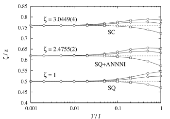
Figure 5: $J^{\prime}$-dependence of the effective coordination number [Eq. (3)] for the SQ, SQ+ANNNI, and SC lattices with $S=1/2$ (squares), 1 (diamonds), and 3/2 (circles). The error bar of each point, except for the exact results for the $S=1/2$ SQ lattice, is much smaller than the symbol size. Horizontal dashed lines denote the limiting value for each lattice evaluated by taking an average of $\zeta(J^{\prime})$ at $J^{\prime}=0.001$, 0.002, and 0.005 for $S=1/2$.

V Mapping to Quantum Ising Model

V.1 Spin-1/2 case

In the weak interchain coupling regime, $J^{\prime}/J\ll 1$, the correlation length along chains grows much faster than in the perpendicular directions as the temperature is decreased, and it reaches the one-dimensional scaling region, described by Eq. (23), well before the correlation in the perpendicular directions starts to develop over more than a few times of the lattice spacing. In such a strongly anisotropic regime, it can be justified to take a continuous limit only in the chain direction, while keeping the lattice in the other directions discrete, without introducing any uncontrollable systematic errors. In this limit, as is well-known, a $d$-dimensional classical Ising model is mapped onto a $(d-1)$-dimensional quantum Ising model in a transverse field and vice versa.Suzuki (1976) In this section, we first consider the mapping of the $S=1/2$ classical Ising model. Generalization for $S\geq 1$ will be separately discussed shortly.

In order to derive an explicit relation between the parameters of the classical and the quantum models, we again introduce the transfer matrix formulation for the $d$-dimensional classical Ising model. The partition function of the $S=1/2$ classical Ising model [Eq. (8)] is expressed as

$$Z=\lim_{M\rightarrow\infty}\text{tr}\,(\bm{T}\bm{D})^{M}.$$ (33)

Here $\bm{T}$ is a $2^{N_{\text{s}}}\times 2^{N_{\text{s}}}$ matrix along chains and is a direct product of local transfer matrices

$$\bm{T}=\bigotimes_{\bm{r}}e^{JS^{z}_{i,\bm{r}}S^{z}_{i+1,\bm{r}}/T}=\bigotimes_{\bm{r}}\left(\begin{array}[]{cc}e^{J/4T}&e^{-J/4T}\\ e^{-J/4T}&e^{J/4T}\end{array}\right)$$ (34)

and $\bm{D}$ is a diagonal matrix representing the Boltzmann weight of each slice

$$\bm{D}=\exp\Big{(}\frac{J^{\prime}}{T}\sum_{\bm{r},\bm{\delta}}S^{z}_{i,\bm{r}}S^{z}_{i,\bm{r}+\bm{\delta}}\Big{)}.$$ (35)

On the other hand, the zero-temperature partition function of the quantum spin-$\frac{1}{2}$ transverse-field Ising model defined on a $(d-1)$-dimensional lattice is written as

$$\begin{split}Z_{\text{q}}&=\lim_{T\rightarrow 0}\text{tr}\,e^{-{\cal H}_{\text{q}}/T}\\ &=\lim_{\Delta\rightarrow 0}\text{tr}\,e^{-\Delta{\cal H}_{\text{t}}}e^{-\Delta{\cal H}_{\text{d}}}e^{-\Delta{\cal H}_{\text{t}}}e^{-\Delta{\cal H}_{\text{d}}}\cdots,\end{split}$$ (36)

where the quantum Hamiltonian

$$\begin{split}{\cal H}_{\text{q}}&={\cal H}_{\text{t}}+{\cal H}_{\text{d}}=-\Gamma\sum_{\bm{r}}\sigma_{\bm{r}}^{x}-K\sum_{\bm{r},\bm{\delta}}\sigma_{\bm{r}}^{z}\sigma_{\bm{r}+\bm{\delta}}^{z}\end{split}$$ (37)

is defined on a $(d-1)$-dimensional lattice which has the same structure as a slice of the classical Ising model under consideration. Here $\sigma^{\alpha}_{\bm{r}}$ ($\alpha=x$, $z$) is a Pauli spin operator.

By identifying $\bm{T}$ and $\bm{D}$ in the classical partition function (33) with $e^{-\Delta{\cal H}_{\text{t}}}$ and $e^{-\Delta{\cal H}_{\text{d}}}$ of the transverse-field Ising model (36) respectively, one can readily obtain the following relations:

$$e^{-J/2T} =\tanh\Delta\Gamma\ \ \text{and}$$ (38)

$$\frac{J^{\prime}}{4T} =\Delta K$$ (39)

between the parameters of the two models, $(J,J^{\prime},T)$ and $(K,\Gamma)$, or

$$e^{-J/2T}=\tanh\frac{J^{\prime}\Gamma}{4KT}\simeq\frac{J^{\prime}\Gamma}{4KT}$$ (40)

by eliminating $\Delta$ in Eqs. (38) and (39). The last equation is valid in the limit of $T/J$, $J^{\prime}/T\rightarrow 0$, and relates the temperature $T$ of the classical model in this limit to the strength of the transverse field $\Gamma$ of the quantum model at the ground state. Especially, the critical points $T_{\text{c}}$ of the former at $J^{\prime}\ll J$ and the quantum critical point $\Gamma_{\text{c}}$ of the latter is identified through

$$e^{-J/2T_{\text{c}}}\simeq\frac{J^{\prime}\Gamma_{\text{c}}}{4KT_{\text{c}}}.$$ (41)

Now we are ready to calculate the effective coordination number (3) in the weak interchain coupling limit. From Eqs. (6) and (41),

$$\begin{split}\zeta(J^{\prime})&=\frac{1}{J^{\prime}\chi^{\text{1d}}(T_{\text{c}}(J^{\prime}))}=\frac{4T_{\text{c}}}{J^{\prime}}e^{-J/2T_{\text{c}}}\\ &\!\!\!\!\underset{J^{\prime}\rightarrow 0}{\longrightarrow}\frac{4T_{\text{c}}}{J^{\prime}}\frac{J^{\prime}\Gamma_{\text{c}}}{4KT_{\text{c}}}=\frac{\Gamma_{\text{c}}}{K}.\end{split}$$ (42)

Thus the effective coordination number converges to a finite value in the $J^{\prime}=0$ limit and its limiting value is exactly given by the quantum critical point, $\Gamma_{\text{c}}/K$, of the corresponding $(d-1)$-dimensional quantum Ising model.

One can indeed confirm that the analytic and numerical results for the renormalized coordination number, $\zeta=1$ and 3.0449(4) for the SQ and SC lattices, in the last section agrees completely with the quantum critical point of the transverse-field Ising model, $\Gamma_{\text{c}}/K=1$ (Ref. Pfeuty, 1970) and 3.0440(7) (Ref. He et al., 1990) or 3.0450(2) (Ref. Hamer, 2000) on the single chain and the isotropic square lattice, respectively. Note that in the argument presented above, we do not assume any exact solutions except for the susceptibility of the genuinely one-dimensional model. Therefore Eq. (42) applies to arbitrary Q1D Ising models in any dimensions. (For example, it applies even to the models with frustration in the transverse directions.)

V.2 General spin cases

One may expect that a spin-$S$ classical Ising model could be similarly mapped onto a quantum Ising model with the identical spin size. However, this is not the case. Such a naive mapping, albeit formally possible, gives no physically meaningful weak interchain coupling limit.

To see the difficulty for $S\geq 1$ more precisely, we consider the $S=1$ case as an example. The $S=1$ local transfer matrix along chains is given by

$$\bm{T}_{\bm{r}}=e^{JS_{i,\bm{r}}^{z}S_{i+1,\bm{r}}^{z}/T}=\left(\begin{array}[]{ccc}e^{J/T}&1&e^{-J/T}\\ 1&1&1\\ e^{-J/T}&1&e^{J/T}\end{array}\right).$$ (43)

If this local transfer matrix is fit by an imaginary-time propagator $\exp(-\Delta{\cal H}_{\text{t,\bm{r}}})$ by the following $S=1$ quantum Hamiltonian:

$${\cal H}_{\text{t,\bm{r}}}=-\Gamma\tau^{x}_{\bm{r}}-D(\tau^{z}_{\bm{r}})^{2}-E(\tau^{x}_{\bm{r}})^{2},$$ (44)

where the $\tau^{\alpha}_{\bm{r}}$ ($\alpha=x$, $z$) is a spin-1 operator, $\Gamma$ the transverse field, and $D$ and $E$ are the longitudinal and transverse crystal fields, respectively, we obtain

$$\Delta\Gamma \simeq\frac{J}{\sqrt{2}T}e^{-J/T},$$ (45)

$$\Delta D \simeq J/T,\ \ \text{and}$$ (46)

$$\Delta E \simeq-4J/T$$ (47)

up to the leading order in $J/T$. In the last equations, however, one should notice that $\Delta\Gamma$ vanishes for $T\ll J$ (so that $\Gamma$ itself can remain finite), whereas both $D$ and $|E|$ diverge even after being multiplied by $\Delta$. This desperate asymptotic behavior of the parameters of the mapped quantum system is due to the vanishing diagonal weight for the $S^{z}=0$ state in the transfer matrix $\bm{T}_{\bm{r}}$.

Although for $S\geq 1$ the weight of the states with $|S^{z}|<S$ becomes exponentially small at low temperatures, disregarding such matrix elements in the transfer matrix will mislead us into an incorrect quantum spin Hamiltonian. In order to handle the anisotropic limit of the high-spin models with care, we introduce a unitary transformation defined below.

As mentioned in Sec. II, only the two largest eigenvalues $\lambda_{1}$ and $\lambda_{2}$ of the local transfer matrix $\bm{T}_{\bm{r}}$ are dominant at low temperatures, and the other $2S-1$ eigenvalues are exponentially small in comparison with $\lambda_{1}$ and $\lambda_{2}$. Now we introduce two column vectors $v_{1}$ and $v_{2}$, which are linear combinations of the eigenvectors $u_{1}$ and $u_{2}$ associated with $\lambda_{1}$ and $\lambda_{2}$, respectively,

$$v_{1} =(u_{1}+u_{2})/\sqrt{2}\ \ \text{and}$$ (48)

$$v_{2} =(u_{1}-u_{2})/\sqrt{2}.$$ (49)

Clearly $v_{1}$ and $v_{2}$ are orthogonal with each other by definition and furthermore they are interchanged by the spin inversion transformation, since $u_{1}$ ($u_{2}$) is symmetric (antisymmetric) under the transformation. This implies that one can interpret $v_{1}$ and $v_{2}$ as “wave functions” of a pseudo $S=1/2$ quantum spin. Indeed, by a local unitary transformation by a matrix $\bm{V}_{\bm{r}}=(v_{1},v_{2},v_{3},\ldots,v_{2S+1})$ with $v_{1}$ and $v_{2}$ introduced above and $v_{i}=u_{i}$ for $i\geq 3$, the local transfer matrix at low temperatures $T\ll J$ is reduced to a $2\times 2$ matrix

$$\begin{split}\bm{V}_{\bm{r}}^{-1}{\bm{T}}_{\bm{r}}\bm{V}_{\bm{r}}&=\begin{pmatrix}\lambda_{+}&\lambda_{-}&&&0\\ \lambda_{-}&\lambda_{+}&&&\\ &&\lambda_{3}&&\\ &&&\ddots&\\ 0&&&&\lambda_{2S+1}\end{pmatrix}\\ &\simeq\begin{pmatrix}\lambda_{+}&\lambda_{-}&&&0\\ \lambda_{-}&\lambda_{+}&&&\\ &&0&&\\ &&&\ddots&\\ 0&&&&0\end{pmatrix},\end{split}$$ (50)

where $\lambda_{\pm}=(\lambda_{1}\pm\lambda_{2})/2$. The whole transfer matrix $\bm{T}=\otimes_{\bm{r}}\bm{T}_{\bm{r}}$ of $(2S+1)^{N_{\text{s}}}\times(2S+1)^{N_{\text{s}}}$ is also reduced to a $2^{N_{\text{s}}}\times 2^{N_{\text{s}}}$ matrix by the global unitary transformation using $\bm{V}=\otimes_{\bm{r}}\bm{V}_{\bm{r}}$. We transform the diagonal matrix $\bm{D}$ at the same time to keep the partition function (33) invariant. Using Eqs. (14)–(17), relevant matrix elements of $\bm{D}$ in this new basis are calculated as

$$\begin{split}&(\bm{V}_{\bm{r}}\otimes\bm{V}_{\bm{r}+\bm{\delta}})^{-1}\bm{D}_{\bm{r},\bm{r}+\bm{\delta}}(\bm{V}_{\bm{r}}\otimes\bm{V}_{\bm{r}+\bm{\delta}})\\ &\qquad\simeq\begin{pmatrix}e^{S^{2}J^{\prime}/T}&&&0&\\ &\!\!\!\!e^{-S^{2}J^{\prime}/T}&&&\\ &&\!\!\!\!e^{-S^{2}J^{\prime}/T}&&\\ 0&&&\!\!\!\!e^{S^{2}J^{\prime}/T}&\\ &&&&\!\!\!\!\ddots\end{pmatrix}.\end{split}$$ (51)

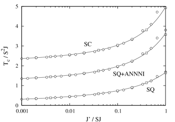
Figure 6: Scaling plot of the critical temperature for the SQ, SQ+ANNNI, and SC lattices with $S=1/2$ (squares), 1 (diamonds), and 3/2 (circles). Solid lines denote scaling function, $2ye^{-2/y}=Cx$, with $x=J^{\prime}/SJ$, $y=T_{\text{c}}/S^{2}J$, and $C=\lim_{J^{\prime}\rightarrow 0}\zeta(J^{\prime})$ [$\approx 1$, 2.4755, and 3.0449 for SQ, SQ+ANNNI, and SC, respectively]. The error bar of each point is much smaller than the symbol size. The data for the SQ+ANNNI and SC lattices are shifted upwards by 1 and 2, respectively, for visibility.

The effective partition function of the spin-$S$ classical Ising model in the weak interchain coupling limit thus becomes equivalent to a spin-1/2 partition function, and then is mapped onto a spin-1/2 quantum Ising model, instead of spin-$S$, as the same as the $S=1/2$ classical Ising model. Noticing that

$$\begin{pmatrix}\lambda_{+}&\lambda_{-}\\ \lambda_{-}&\lambda_{+}\end{pmatrix} =\exp\begin{pmatrix}\log(\lambda_{+}-\lambda_{-})&\frac{1}{2}\log\frac{\lambda_{+}+\lambda_{-}}{\lambda_{+}-\lambda_{-}}\\ \frac{1}{2}\log\frac{\lambda_{+}+\lambda_{-}}{\lambda_{+}-\lambda_{-}}&\log(\lambda_{+}-\lambda_{-})\end{pmatrix}$$ (52)

$$=\exp\begin{pmatrix}\log\lambda_{1}&\frac{1}{2}\log\lambda_{1}/\lambda_{2}\\ \frac{1}{2}\log\lambda_{1}/\lambda_{2}&\log\lambda_{1}\end{pmatrix},$$ (53)

one can explicitly write down the correspondence between the spin-$S$ classical Ising model and the spin-1/2 quantum transverse-field Ising model as

$$\log\frac{\lambda_{1}(T)}{\lambda_{2}(T)} \equiv 1/\xi_{\text{1d}}(T)=2\Delta\Gamma\ \ \text{and}$$ (54)

$$\frac{S^{2}J^{\prime}}{T} =\Delta K$$ (55)

or

$$1/\xi_{\text{1d}}(T) =\frac{2S^{2}J^{\prime}\Gamma}{KT}$$ (56)

for $J^{\prime}\ll T\ll J$. Furthermore, using the low-temperature asymptotic form for the correlation length of a single chain [Eq. (23)], we obtain a relation between the classical and the quantum critical point parameters as

$$e^{-2S^{2}J/T_{\text{c}}}\simeq\frac{SJ^{\prime}\Gamma_{\text{c}}}{2T_{\text{c}}K},$$ (57)

which reduces to Eq. (41) for $S=1/2$. The last equation suggests that two dimensionless variables, $x\equiv J^{\prime}/SJ$ and $y\equiv T_{\text{c}}/S^{2}J$, satisfy a scaling relation, $2ye^{-2/y}=Cx$ with an $S$-independent constant $C=\Gamma_{\text{c}}/K$. In Fig. 6, this scaling relation is tested explicitly by using the Monte Carlo results in the last section. For each lattice the data in the weak interchain coupling regime $J^{\prime}/SJ\lesssim 0.1$ collapse on a single curve as expected from the scaling form (57).

Finally, using Eq. (24), the effective coordination number in the $J^{\prime}/J=0$ limit is obtained as $C=\Gamma_{\text{c}}/K$, irrespective of the spin size, which is a proof of the $S$-independent renormalization of the coordination number suggested by the Monte Carlo simulation in the last section. One should note the nontrivial factor $1/S$ in the scaling variable $x=J^{\prime}/SJ$, which cancels with the same factor in the scaling form for the single-chain susceptibility [Eq. (24)] to make the effective coordination number independent of $S$. We also emphasize that our final result, $\zeta(J^{\prime})\rightarrow\Gamma_{\text{c}}/K$, does not depend on the scaling conjecture for the susceptibility and correlation length of a single chain; it can be deduced more directly from Eqs. (20) and (56) instead.

VI Summary and Discussion

In this paper we presented our detailed analysis on the critical temperature and the effective coordination number of the Q1D general-spin Ising ferromagnets. The critical temperature is estimated down to $J^{\prime}/J=0.001$ with high accuracy by the cluster Monte Carlo method performed on infinite-length strips. It is demonstrated that as the interchain coupling is decreased the effective coordination number converges to a finite value $\zeta$, which is definitely less than the coordination number $z$, quite rapidly. Furthermore, we show unambiguously that the renormalized coordination number is independent of the spin size $S$. This is the same as the observation for the Q1D and Q2D quantum Heisenberg antiferromagnets, reported in Ref. Yasuda et al., 2005, and thus is expected to be observed widely in other classes of quasi-low-dimensional magnets.

We explain the origin of the renormalization of the effective coordination number by considering a mapping to quantum Ising models, where the spin-$S$ classical Ising model is rigorously shown to be mapped onto a spin-$1/2$ quantum transverse-field Ising model, irrespective of the spin size $S$, in the weak interchain coupling limit, and the effective coordination number is given by the quantum critical point $\Gamma_{\text{c}}/K$ of the mapped quantum Ising model. It should be noticed that in the scaling relation of the critical temperature [Eq. (57)], a nontrivial factor $1/S$ appears, which cannot be deduced by a naive dimensional analysis. This factor cancels out with another nontrivial factor in the single-chain susceptibility [Eq. (24)], and then results in an $S$-independent scaling relation. Another remarkable fact to be noticed is that corrections to the asymptotic value in the effective coordination number are much smaller than those in the single-chain susceptibility itself, which suggests existence of a more fundamental theory, describing the critical temperature of strongly anisotropic magnets, than the modified CMF relation, Eq. (2) combined with $z=\zeta$.

The renormalized coordination number is, however, found to be nonuniversal with respect to the lattice structure. This is natural from the viewpoint of the mapped quantum Ising model, where the critical transverse field of a quantum critical point cannot be a universal quantity; it depends on the fine lattice structure as well as on the details of interaction. Thus an introduction of a weak further neighbor interaction or an anisotropy in slices, for example, will modify the renormalized coordination number. In this sense, the “universality,” discussed in the present paper, is different from that asserted for critical exponents in usual continuous phase transitions and thus inexact terminologically.

Finally, we emphasize again that the weak interchain coupling limit of the Q1D classical Ising model is not the weak coupling limit ; it is still in the strongly correlated regime, i.e., in the vicinity of a quantum critical point, of the mapped quantum Ising model. This explains why the CMF approximation remains inaccurate even in this limit. We expect a similar argument will apply to the Q1D and Q2D quantum Heisenberg models. It is unclear and remains as an open problem, however, whether it is possible to generalize the present mapping approach to the quantum Heisenberg models, where a continuous axis, the imaginary-time axis, exists intrinsically, and therefore extra care should be necessary to introduce another continuous axis representing a strong spatial anisotropy.

References

- Scalapino et al. (1975) D. J. Scalapino, Y. Imry, and P. Pincus, Phys. Rev. B 11, 2042 (1975).
- Schulz (1996) H. J. Schulz, Phys. Rev. Lett. 77, 2790 (1996).
- Yasuda et al. (2005) C. Yasuda, S. Todo, K. Hukushima, F. Alet, M. Keller, M. Troyer, and H. Takayama, Phys. Rev. Lett. 94, 217201 (2005).
- Irkhin and Katanin (1997) V. Y. Irkhin and A. A. Katanin, Phys. Rev. B 55, 12318 (1997).
- Irkhin and Katanin (1998) V. Y. Irkhin and A. A. Katanin, Phys. Rev. B 57, 379 (1998).
- Irkhin et al. (1999) V. Y. Irkhin, A. A. Katanin, and M. I. Katsnelson, Phys. Rev. B 60, 1082 (1999).
- Irkhin and Katanin (2000) V. Y. Irkhin and A. A. Katanin, Phys. Rev. B 61, 6757 (2000).
- Bocquet (2002) M. Bocquet, Phys. Rev. B 65, 184415 (2002).
- Hastings and Mudry (2006) M. B. Hastings and C. Mudry, Phys. Rev. Lett. 96, 027215 (2006).
- (10) A. Praz, C. Mudry, and M. B. Hastings, cond-mat/0606032.
- (11) D. X. Yao and A. W. Sandvik, cond-mat/0606341.
- Onsager (1944) L. Onsager, Phys. Rev. 65, 117 (1944).
- Kramers and Wannier (1941) H. A. Kramers and G. H. Wannier, Phys. Rev. 60, 252 (1941).
- Suzuki et al. (1967) M. Suzuki, B. Tsujiyama, and S. Katsura, J. Math. Phys. 8, 124 (1967).
- Swendsen and Wang (1987) R. H. Swendsen and J. S. Wang, Phys. Rev. Lett. 58, 86 (1987).
- Wolff (1989) U. Wolff, Phys. Rev. Lett. 62, 361 (1989).
- Matsumoto et al. (2001) M. Matsumoto, C. Yasuda, S. Todo, and H. Takayama, Phys. Rev. B 65, 014407 (2001).
- Evertz and von der Linden (2001) H. G. Evertz and W. von der Linden, Phys. Rev. Lett. 86, 5164 (2001).
- Todo and Kato (2000) S. Todo and K. Kato, Prog. Theor. Phys. Suppl. 138, 535 (2000).
- Todo and Kato (2001) S. Todo and K. Kato, Phys. Rev. Lett. 87, 047203 (2001).
- Ferrenberg and Landau (1991) A. M. Ferrenberg and D. P. Landau, Phys. Rev. B 44, 5081 (1991).
- Cardy (1984) J. L. Cardy, J. Phys. A: Math. Gen. 17, L385 (1984).
- Butera et al. (2003) P. Butera, M. Comi, and A. J. Guttmann, Phys. Rev. B 67, 054402 (2003).
- Suzuki (1976) M. Suzuki, Prog. Theor. Phys. 56, 1454 (1976).
- Pfeuty (1970) P. Pfeuty, Ann. Phys. 57, 79 (1970).
- He et al. (1990) H.-X. He, C. J. Hamer, and J. Oitmaa, J. Phys. A: Math. Gen. 23, 1775 (1990).
- Hamer (2000) C. J. Hamer, J. Phys. A: Math. Gen. 33, 6683 (2000).
- (28) http://alps.comp-phys.org.
- Alet et al. (2005) F. Alet, P. Dayal, A. Grzesik, A. Honecker, M. Körner, A. Läuchli, S. R. Manmana, I. P. McCulloch, R. M. Noack, G. Schmid, et al., J. Phys. Soc. Jpn. Suppl. 74, 30 (2005).