Study of the one dimensional Holstein model using the augmented space approach

Abstract

A new formalism using the ideas of the augmented space recursion (introduced by one of us) has been proposed to study the ground state properties of ordered and disordered one-dimensional Holstein model. For ordered case our method works equally well in all parametric regime and matches with the existing exact diagonalization and DMRG results. On the other hand the quenched substitutionally disordered model works in low and intermediate regime of electron phonon coupling. Effect of phononic and substitutional disorder are treated on equal footing.

1 Introduction

When a conduction electron or hole moves through a polar crystal it polarizes and distorts the neighboring ion lattice sites. When it moves it carries along with it the lattice distortion. The electron together with this lattice distortion or self-consistent polarization field is a quasi particle and is referred to as polaron. Many experiments indicate strong evidence of polaronic carriers in strongly correlated electronic materials like manganites (showing colossal magneto-resistance) [1]-[2], organic [3] and high $T_{c}$ superconducting cuprates [4]-[5]. Holstein model[6] has been one of the basic model used to study the formation and nature of polaron. Analytical approaches to solve the model have got limited success. Main draw back of those results are they are valid only in a limited range of parametric regime of electron-phonon coupling [7] and also for small system size.

Recently there has been a spurt in numerical studies on this model, which includes the variational approach based on exact diagonalization method (VAED) [8]-[9], the density-matrix renormalization group techniques (DMRG) [12], exact diagonalization techniques(ED) [13]-[19], the quantum Monte Carlo calculations (QMC) [20]-[21] and global-local method [22]. None of these methods work equally well in all parametric regimes. Each has some shortcomings. VAED, the most recent and successful of the methods, though highly accurate in the the weak and intermediate coupling regimes, fails to maintain its accuracy in the strong coupling limit. The DMRG method is accurate in the strong and intermediate coupling regimes, but is not accurate in the weak coupling regime. The DMRG results are not translationally symmetric. DMRG lacks the accuracy of VAED in the weak coupling regime because its lattice size is smaller than the spatial extent of the large polaron that will be formed. The VAED cannot emulate its success of the low and intermediate regime in the the strong coupling regime because the electron-phonon system demands more phonons in its ‘root state’ [9] and its near vicinity.

Disordered Holstein model has been earlier attempted by [10] using Dynamical CPA. But their method is effective in the intermediate electron-phonon coupling regime and for only infinite coordination, i.e. on a Bethe Lattice. Keeping this in mind, in this communication we have proposed a reciprocal space recursion technique, introduced earlier by us in a different context [11], as a feasible method for the study of the Holstein model. We have constructed a basis which meets the requirement in all parametric regimes.

2 The Augmented Space Formalism for ordered Holstein model

In this section we shall describe the setting up of the electron-phonon Hamiltonian as an operator on the underlying Hilbert space. The electronic part will be represented in a tight-binding like basis. In our simple model there will be only a single orbital per site and the tight-binding basis will be labeled by a site $R_{n}$ : $\{|R_{n}\rangle\}$. This basis will span the electronic part of the Hilbert space ${\bf H}^{el}$. The phonon part will be described by a configuration state which will indicate how many phonon excitations there are at each site labeled by $R_{n}$. Each configuration will be a pattern of the type $\{n_{R_{1}},n_{R_{2}}\ldots n_{R_{n}}\ldots\}$ where $n_{R_{n}}$ takes the values $0,1,2,\ldots$ and is called the cardinality of the site $R_{n}$. The pattern is called the cardinality sequence and uniquely labels a phonon state. These states will span the phonon part of the Hilbert space ${\bf H}^{ph}$. The total Hilbert space of states of the electron-phonon system will be ${\bf H}\ =\ {\bf H}^{el}\otimes{\bf H}^{ph}$. A member of the basis in this product space will be labeled both by the site labeled real-space part and a configuration part which tells us how many local phononic excitations are there at each site in the lattice, e.g. $|R_{n}\otimes\{n_{R_{1}},n_{R_{2}},\ldots\}\rangle$.

In this basis, the Holstein Hamiltonian [6] is :

$$H=\ \varepsilon\sum_{R_{n}}P_{n}\otimes{I}-t\sum_{R_{n}}\sum_{R_{m}}T_{nm}\otimes\ {I}+\hbar\omega\sum_{R_{n}}I\otimes{N}_{n}-\lambda\sum_{R_{n}}P_{n}\otimes\left({T}_{n}^{+}+{T}_{n}^{-}\right)$$ (1)

where,

• $P_{n}$ is the projection operator $|R_{n}\rangle\langle R_{n}|$ and $T_{nm}=|R_{n}\rangle\langle R_{m}|$ is the transfer operator in the electronic part of the Hilbert space ${\bf H}^{el}$,

• ${T}_{n}^{\pm}=|\ldots n_{R_{n}}\pm 1\ldots\rangle\langle\ldots n_{R_{n}}\ldots|$ are the step up or step down operators and ${N}_{n}$ is the number operator $n_{R_{n}}|\ldots n_{R_{n}}\ldots\rangle\langle\ldots n_{R_{n}}\ldots|$ both in the phononic part of the Hilbert space ${\bf H}^{ph}$.

• Here a single electron with an on-site energy $\varepsilon$ can hop to its near neighbour on an infinite lattice with hopping integral $t$ and interacts with dispersion less optical phonons with frequency $\omega$. The electron-phonon coupling strength is denoted by $\lambda$ . The parameters $\varepsilon$,$t$, $\hbar\omega$ and $\lambda$ have the units of energy.

• In all subsequent calculations energies are scaled in units of t.

This type of Hamiltonian in an augmented space ${\bf H}^{el}\otimes{\bf H}^{ph}$ has been introduced earlier by us [23] to deal with time dependent disorder in an electronic system, precisely of the form produced by lattice vibrations. The great advantage of this formulation is that if we have quenched disorder in $\varepsilon(R_{n})$, then a simple augmentation of the Hilbert space ${\bf H}^{el}$ by the configuration space of the $\varepsilon(R_{n})$ allows us to deal with all the configuration averaged properties of a disordered Holstein model. This extension will be carried out by us in a later section. Since we are interested in calculating the spectral function, dispersion curves of the system, we generalize the above mentioned formalism to generate basis states in reciprocal space. Here a general state in the augmented reciprocal-space basis has the following form :

$$|k\otimes\{n_{R_{1}},n_{R_{2}}\ldots n_{R_{n}}\ldots\}\rangle=(1/\sqrt{N})\sum_{R_{n}}\mbox{exp}(ik\cdot R_{n})|R_{n}\otimes\{n_{R_{1}},n_{R_{2}}\ldots n_{R_{n}}\ldots\}\rangle.$$

Here $k$ is a reciprocal space vector and we have Fourier transformed the electronic part of the basis to momentum space keeping the bosonic part unchanged. In the recursion method, which we shall later employ, we shall generate the basis states by repeatedly applying the Hamiltonian on the following starting state :

$$|1\rangle=|k\otimes\{\emptyset\}\rangle=(1/\sqrt{N})\sum_{R_{n}}\exp\{ik\cdot R_{n}\}|R_{n}\otimes\{\emptyset\}\rangle$$

Here $\{\emptyset\}$ denotes a zero phonon configuration in the bosonic subspace of the full Hamiltonian. That is, with a null cardinality sequence.

Alternatively, we can generate basis states recursively by similar action of the Hamiltonian on the following two states :

1. $$|1\rangle=|k\otimes\{\emptyset\}\rangle=(1/\sqrt{N})\sum_{R_{n}}\exp\{ik\cdot R_{n}\}|R_{n}\otimes\{\emptyset\}\rangle$$

2. $$|2\rangle=|k\otimes\{N_{1},0,0\ldots\}\rangle=(1/\sqrt{N})\sum_{R_{n}}\exp\{ik\cdot R_{n}\}|R_{n}\otimes\{N_{1},0,0\ldots\}\rangle$$

Here ${N_{1},0,0..}$ denotes $N_{1}$ number of phonon at site $1$ of the bosonic subspace of the Hamiltonian and zero else where. We shall call this the phonon-enriched state.

The advantage of the second choice is that, if we apply the Hamiltonian $N$ times on the two initial states, $N+N_{1}$ number of phonons are generated in the site $1$ and sufficient number of bosons are generated in its vicinity, while in the first choice we get only $N$ number of phonons in the first site and progressively less numbers in the neighboring sites. This is important in order to get a convergent result in the high e-ph coupling regime.

In order to calculate averaged spectral function we tri-diagonalize the Hamiltonian using the following three term recursion  :

We start from a state $|k\otimes\{n_{R_{1}},\ldots\}\rangle\ =\ |1\rangle$ and generate the other states through the following three term recursion :

$$|n+1\rangle=H|n\rangle-\alpha_{n}(k)|n\rangle-\beta^{2}_{n-1}(k)|n-1\rangle$$ (2)

The coefficients $\alpha_{n}(k)$ and $\beta^{2}_{n}(k)$ are obtained by ensuring that the new basis generated is orthogonal. This yields :

$$\alpha_{n}(k)=\langle n|H|n\rangle/\langle n|n\rangle\quad\quad\beta_{n}^{2}(k)=\langle n+1|n+1\rangle/\langle n|n\rangle$$

To carry out the recursion we need to know the action of the Hamiltonian (1) on a general state : If write the Hamiltonian (1) as : $H=H_{1}+H_{2}+H_{3}+H_{4}$ then

$$H_{1}|k\otimes\{n_{R_{1}},n_{R_{2}}\ldots\}\rangle = \varepsilon|k\otimes\{n_{R_{1}},n_{R_{2}}\ldots\}\rangle$$

$$H_{2}|k\otimes\{n_{R_{1}},n_{R_{2}}\ldots\}\rangle = -t\sum_{\chi}\exp\{ik\cdot\chi\}|k\otimes\{n_{R_{1}-\chi},n_{R_{2}-\chi}\ldots\}\rangle$$

$$H_{3}|k\otimes\{n_{R_{1}},n_{R_{2}}\ldots\}\rangle = \left(\rule{0.0pt}{8.53581pt}\hbar\omega\sum_{n}n_{R_{n}}\right)|k\otimes\{n_{R_{1}},n_{R_{2}}\ldots\}\rangle$$

$$H_{4}|k\otimes\{n_{R_{1}},n_{R_{2}}\ldots\}\rangle = -\lambda|k\otimes\{n_{R_{1}}\pm 1,n_{R_{2}},\ldots\}\rangle$$ (3)

Once we carry out a recursive determination of the coefficients $\{\alpha_{n}(k),\beta^{2}_{n}(k)\}$, the Green function is given as a continued fraction :

$$G(k,E)=\frac{1}{\displaystyle E-\alpha_{1}(k)-\frac{\beta_{1}^{2}(k)}{\displaystyle E-\alpha_{2}(k)-\frac{\beta_{2}^{2}(k)}{\displaystyle{{\ddots}\atop{\displaystyle{\frac{\beta_{N-1}^{2}}{\displaystyle{E-\alpha_{N}(k)-\beta_{N}^{2}(k)\ T(k,E)}}}}}}}}$$

We carry out recursion up to a finite number of N steps and then terminate the continued fraction with a herglotz terminator $T(k,E)$ [26] suggested by Beer and Pettifor [27]. The spectral function is then given by :

$$A(k,E)=-(1/\pi)\Im m\ll G(k,E)\gg$$

The dispersion curves are obtained by fitting Lorentzian’s in the neighbourhood of the peaks in the spectral function : the Lorentzian centre gives the energy $E(k)$ while the width gives the width in the dispersion curves.

We apply the recursion based conjugate gradient (CG) technique [25] to obtain ground state energy and wave function. To calculate the excited state wave function we find a orthogonal state to the ground state using Gram-Schmidt method of orthogonalization and then apply CG technique to find the first excited state energy and wave function. With the wave function and dispersion curve at our disposal we find the various correlation functions,effective mass from it. The effective mass we have calculated using the standard formula :

$$\frac{m_{0}}{m_{*}}=\left.\frac{1}{2t}\frac{\partial^{2}E(k)}{\partial k^{2}}\right|_{k=0}$$ (4)

The mean phonon number indicates a measure of the phononic character of the polaron.

$$N^{ph}\ =\langle\psi_{0}|I\otimes{N}_{n}|\psi_{0}\rangle$$ (5)

Here $|\psi_{0}\rangle$ is the ground state wave function obtained from the CG technique. The static correlation function between the electron position and oscillator displacement is given

$$\chi(R_{i}-R_{j})=\langle\psi_{0}|P_{i}\otimes({T}_{j}^{+}+{T}_{j}^{-})|\psi_{0}\rangle$$ (6)

The number of excited phonons in the vicinity of the electron is given by

$$\gamma(R_{i}-R_{j})=\langle\psi_{0}|P_{i}\otimes{N}_{j}|\psi_{0}\rangle$$ (7)

3 Augmented space formalism for disordered Holstein model

In this section we shall generalize our ideas to a disordered Holstein model. We shall start with a Hamiltonian :

$$H=\ \sum_{R_{n}}\varepsilon(R_{n})P_{n}\otimes{I}-t\sum_{R_{n}}\sum_{R_{m}}T_{nm}\otimes\ {I}+\hbar\omega\sum_{R_{n}}I\otimes{N}_{n}-\lambda\sum_{R_{n}}P_{n}\otimes\left({T}_{n}^{+}+{T}_{n}^{-}\right)$$

where,

$$\varepsilon(R_{n})=\varepsilon_{A}\ n(R_{n})+\varepsilon_{B}\ (1-n(R_{n}))$$

Here $n(R_{n})$ is a random variable which takes the value 0 if $R_{n}$ is occupied by an A type of atom and 1 if it is occupied by a B type. The probability of these events are $x$ (the concentration of A atoms in the alloy) and $1-x$ (concentration of B atoms in the alloy) respectively. IN this simple model we shall consider only this type of binary substitutional disorder. For real disordered alloys the other parameters $t$, $\omega$ and $\lambda$ may also be random. The augmented space formalism for quenched disorder [28] writes the probability density of the random variables as :

$${P}[n(R_{n})] = x\ \delta[n(R_{n})-1]+(1-x)\ \delta[n(R_{n})]$$

$$= -(1/\pi)\ \Im m\ \langle\uparrow|\left((n(R_{n})+i\delta){I}-{M}^{(n)}\right)^{-1}|\uparrow\rangle$$

The operator M⁽ⁿ⁾ associated with the random variable $n(R_{n})$ is such that its spectral density is the probability density of the random variable. Here the representation of this operator is

$${M}^{(n)}\ =\ \left(\begin{array}[]{cc}x&\sqrt{x(1-x)}\\ \sqrt{x(1-x)}&1-x\end{array}\right)$$

in the basis $|\!\uparrow\rangle=\sqrt{x}|0\rangle+\sqrt{1-x}|1\rangle$ and $|\!\downarrow\rangle=\sqrt{1-x}|0\rangle-\sqrt{x}|1\rangle$, where $|0\rangle$ and $|1\rangle$ are the eigenvectors of M⁽ⁿ⁾ with eigenvalues 0 and 1 respectively.

The configuration space of a single random variable $n(R_{n})$ : $\phi^{(n)}$ is of rank 2 and is spanned by these vectors $|\uparrow\rangle$ and $|\downarrow\rangle$ and M⁽ⁿ⁾ is an operator on this space. We consider the configuration space of all the variables $\{n(R_{n})\}$ : $\Phi=\prod^{\otimes}\phi^{(n)}$. The augmented space formalism [28] constructs a Hamiltonian :

$$\widetilde{H} = \ \ll\varepsilon\gg\sum_{R_{n}}P_{n}\otimes{I}\otimes{I}+\varepsilon_{1}\sum_{R_{n}}P_{n}\otimes{I}\otimes P^{n}_{\downarrow}+\varepsilon_{2}\sum_{R_{n}}P_{n}\otimes{I}\otimes T^{n}_{\uparrow\downarrow}$$ (8)

$$-t\sum_{R_{n}}\sum_{R_{m}}T_{nm}\otimes\ {I}\otimes I+\hbar\omega\sum_{R_{n}}I\otimes{N}_{n}\otimes I-\lambda\sum_{R_{n}}P_{n}\otimes\left({T}_{n}^{+}+{T}_{n}^{-}\right)\otimes I$$

where,

• $P^{n}_{\downarrow}=|\downarrow^{n}\rangle\langle\downarrow^{n}|$ and $T^{n}_{\uparrow\downarrow}=|\uparrow^{n}\rangle\langle\downarrow^{n}|+|\downarrow^{n}\rangle\langle\uparrow^{n}|$ are the projection and transfer operators in the configuration space $\Phi$

• $\epsilon_{1}=(1-x)(\varepsilon_{A}-\varepsilon_{B})$ and $\varepsilon_{2}=\sqrt{x(1-x)}(\varepsilon_{A}-\varepsilon_{B})$.

This enlarged Hamiltonian is in the full augmented Hilbert space :  $\widetilde{\bf H}={\bf H}^{el}\otimes{\bf H}^{ph}\otimes\Phi$. As in the case of the phonon space, in this disorder configuration space, a general vector is a pattern of $\uparrow$ and $\downarrow$-s. The sequence of sites where we have a $\downarrow$ is called the cardinality sequence and uniquely describes the configuration. A typical member of a basis in this augmented space is $|R_{j}\otimes\{n_{R_{1}},n_{R_{2}},\ldots\}\otimes\{R_{k_{1}},R_{k_{2}},\ldots\}\rangle$.

The augmented space theorem [28] states that :

$$\ll G(R,E)\gg=\langle R\otimes\{\emptyset\}\otimes\emptyset|\ \left(E\tilde{I}-\widetilde{H}\right)^{-1}\ |R\otimes\{\emptyset\}\otimes\emptyset\rangle$$ (9)

where $|\emptyset\rangle\ \epsilon\ \Phi$ is the null cardinality sequence or one where we have $\uparrow$ everywhere. Equivalently, exactly as discussed in section 1, we can construct the above formalism in reciprocal space by Fourier transforming the electronic part of the basis and keeping the rest unchanged. So we can write the configuration averaged Green’s function in reciprocal space as :

$$\ll G(k,E)\gg=\langle k\otimes\{\emptyset\}\otimes\emptyset|\ \left(E\tilde{I}-\widetilde{H}\right)^{-1}\ |k\otimes\{\emptyset\}\otimes\emptyset\rangle$$ (10)

The operation of the terms in the Hamiltonian are mostly identical to (7) except for the second to fourth terms in equation (8) :

$$\widetilde{H}_{2}|k\otimes\{n_{R_{1}},\ldots\}\otimes\{{\bf C}\}\rangle\ = \ \varepsilon_{1}\ \delta(R_{1}\in\{{\bf C}\})\ |k\otimes\{n_{R_{1}},\ldots\}\otimes\{{\bf C}\}\rangle$$

$$\widetilde{H}_{3}|k\otimes\{n_{R_{1}},\ldots\}\otimes\{{\bf C}\}\rangle\ = \ \varepsilon_{2}\ |k\otimes\{n_{R_{1}},\ldots\}\otimes\{{\bf C}\pm R_{1}\}\rangle$$

$$\widetilde{H}_{4}|k\otimes\{n_{R_{1}},\ldots\}\otimes\{{\bf C}\}\rangle\ = \ -t\sum_{\chi}\exp\{ik\cdot\chi\}|k\otimes\{n_{R_{1}}-\chi\ldots\}\otimes\{{\bf C}-\chi\}\rangle$$

here, $\{{\bf C}\}$ is a general cardinality sequence $\{R_{k},R_{m},\ldots\}$.

For obtaining the configuration averaged spectral function we carry out recursion with the starting state $|k\otimes\{n_{R_{1}},\ldots\}\otimes\emptyset\rangle\ =\ |1\rangle$ using the three term recursion similar to (6) but in the full augmented space. As before, from the orthogonality of the recursive states, we obtain the coefficients $\tilde{\alpha}(k),\tilde{\beta}(k)$ and averaged Green function is obtained as a continued fraction :

$$\ll G(k,E)\gg=\frac{1}{\displaystyle E-\tilde{\alpha}_{1}(k)-\frac{\tilde{\beta}^{2}_{1}(k)}{\displaystyle E-\tilde{\alpha}_{2}(k)-\frac{\tilde{\beta}_{2}^{2}(k)}{\displaystyle{{\ddots}\atop{\displaystyle\frac{\beta_{N-1}^{2}}{\displaystyle E-\alpha_{N}-\beta_{N}^{2}\ \tilde{T}(k,E)}}}}}}$$ (12)

As before the calculation is carried down to a finite number N of steps and then the continued fraction is terminated by a function $\tilde{T}(k,E)$ as suggested by Beer and Pettifor. The configuration averaged spectral function and other quantities of interest are calculated using the same formalism as discussed in section 1.

4 The Ground state in a ordered Holstein model

In this section we will discuss the results of our ground-state properties and compare them with the results of two of the most successful recent numerical works.

The figure 1 shows the spectral functions for different $k$ values. All the spectral functions show a very narrow delta function like peaks at the lower end of the spectrum. This is related to the band corresponding to the polaron ground state. This state has very narrow width, which means this $k$-labeled state has a very long lifetime. The other peaks are related to excited states. These have larger widths.

The dispersion curves shown in figure 2 (left) are obtained by fitting Lorentzian’s in the neighbourhood of the peaks in the spectral function : the Lorentzian centre gives the energy $E(k)$ while the width gives the width in the dispersion curves.

Table-I compares our polaron ground-state energy at k=0 with those obtained by VAED [8] (in the weak coupling regime) and DMRG [12] (in the Strong coupling regime) for two sets of parameters. The ground state energies were obtained by two different starting root states as mentioned earlier. Our energies match extremely well with both the earlier VAED and DMRG calculations.

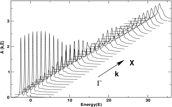
Figure 1: The spectral functions are plotted for different $k$ values. The spectral functions are obtained from a k-space recursion with a 22 shell nearest neighbour map.

$\lambda/\omega$	Present(VAED)	Present(M-VAED)	VAED[8]	DMRG[12]
1.0	-2.469684723933	-2.469684723933	-2.469684723933	-2.46968
$\sqrt{2}$	-2.998828186866	-2.998828186866	-2.998828186867	-2.99883

Table 1: Comparison of Polaron Ground state energy for k=0 for two different parameters. M-VAED refers to the phonon enriched starting state described in section 1

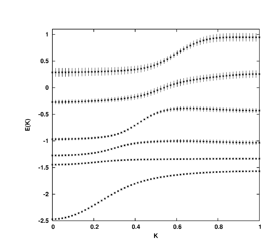
Figure 2: (left) Dispersion curves for ground state and few excited states are plotted for $\lambda=\omega=1$. The recursion was carried out using a 22 shell map. (right) Dispersion curves for different values of e-ph coupling. Here $\lambda/\omega$ = g

Figure 3: The left panel shows the logarithm of the ratio of the polaronic mass $m^{*}$ to bare electron mass w.r.t. the electron-phonon coupling strength in different Limits. Dots are the DMRG extracted data points and Squares are VAED extracted data points. The right panel shows the average kinetic energy for different values of $\omega$

We have calculated the effective mass spanning all parametric regimes. We find good agreement with results of the DMRG and the earlier VAED methods. This is shown in figure 3(left panel). To check numerical stability we have done the calculations first with a 17 shell map with a maximum of 34 phonons and another with a 18 shell map with a maximum of 35 phonons. The results match to within our accuracy window across the parametric regime $0\leq g\leq 5$. At the low electron-phonon coupling regime we have a quasi-free electron with a slightly renormalized mass. As the electron-phonon coupling strength increases the polaron becomes heavier. The crossing though always smooth, is rapid in the adiabatic limit. In the same figure(right panel) we also plot the averaged kinetic energy, which rapidly decreases as the polaron becomes heavier .

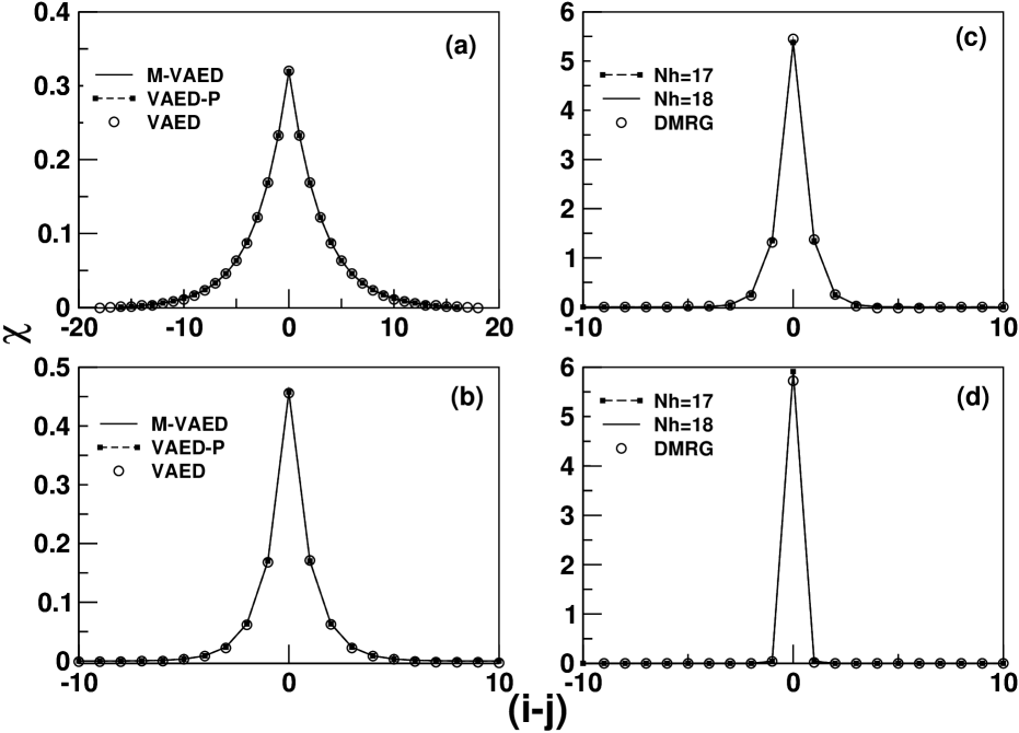
Figure 4: The Lattice deformation $\chi$ as function of $R_{i}-R_{j}$ at k=0 for (a) $\omega$=.1 and$\lambda$=.1, (b)$\omega$=1. and $\lambda$=.5, (c)$\omega$=.1 and$\lambda$=.435, (d)$\omega$=1. and $\lambda$=3.

We have calculated the static correlation function $\chi(R_{i}-R_{j})$ between the electron position and quanta of lattice vibration which gives us a measure of the electron-induced lattice deformation and its spatial extent. We compare our results with VAED and DMRG results. There is excellent agreement in between our results generated using both of our basis and VAED results which is shown in figure 4. In figure 4(a) we show the static correlation function for $\omega$=0.1 (adiabatic) and $\lambda$=0.1(weak coupling), and we can clearly see spatial extent of the polaron span the system size, therefore a large polaron. We do not show the DMRG result in this case as it is less reliable in this parameter regime. In figure4(b) we show the $\chi$ for $\omega$=1.0 and $\lambda$=0.5, which again matches well with the VAED calculation. Figure4(c) and figure4(d) give us the result for high electron-phonon coupling in adiabatic $\omega/t$=0.1 ($\lambda$=4.35) and intermediate $\omega/t$=1.0($\lambda$=3.0) limits respectively. In both the cases spatial extent of the polaron has been reduced, resulting in small polaron. Here we have achieved excellent convergence applying the modified or phonon-enriched VAED basis (M-VAED), as described in section 1, using N=17 (34 bosons at the root site); N=18 (36 phonons at root site) and N=19 (37 phonons at the root site) shell maps. Our energy converges to 11-12 decimal places for these two calculations. Figure4(c) shows good agreement with DMRG results. The value of our extracted DMRG $\chi$(0) is 5.459016. The value of our $\chi(0)$ for this case is 5.374, which is very close to 5.4 the lower limit of extrapolated VAED data. Figure4(d) also has a good agreement with DMRG results. The value of our $\chi$(0) is 5.91 and value of the DMRG extracted data is 5.73. For small polaron our data are in good agreement with DMRG data. Unlike DMRG results , our results are reflection symmetric (i.e.,$\chi$(l)=$\chi$(-l)) as this basis takes proper care of translation symmetry. We conclude that we have achieved highly reliable results in all regimes.

We have also calculated $\chi$ at non-zero k at $\omega$=0.8, $\lambda^{2}$=0.4 (figure 5, left) and $\omega$=1.0, $\lambda$=3.0(figure 5,right) to see how the polaron transforms from predominantly electronic character at k=$0$ to phononic at k=$\pi$. In figure 5(left) at k=0 where group velocity is zero the deformation affects only the sites in its close vicinity , falls off exponentially and is always positive. At k=$\pi/4$, there is a enhancement in the deformation amplitude and it acquires a negative sign in oscillation as well. At k=$\pi/2$ the oscillations are enhanced in sign as well as spatial extent. The spatial extent of the deforming oscillations attains its maximum at k=$\pi$. Our calculation matches well with VAED for same set of parameters for zero as well as non-zero k-values.

XXX

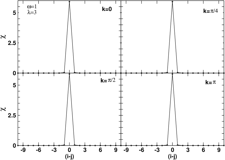
Figure 5: (left) Figure shows lattice deformation $\chi$ for different k values at $\omega=0.8$ and $\lambda^{2}=0.4$. (right) Figure shows lattice deformation $\chi$ for different k values at $\omega=1.0$ and $\lambda=3.0$

Figure 5 (right) shows the $\chi$ for same k-values but for high electron-phonon coupling strength. Here $\chi$ shows hardly any variation with k, i.e., lattice distortion is predominantly on the electron site, with hardly any group velocity. Figure 2 (right panel) shows polaron is almost dispersion less for this parameter i.e., group velocity(${d\omega}/{dk}$) is almost zero and again the average kinetic energy(figure 3 right panel) also drops drastically for this value, hinting clearly that a very small polaron has formed.

We have also calculated the correlation functions $\chi$(0), $\chi$(1), ($\chi$(0)-$\chi$(1))/g which is shown in figure 6. Where g is $\lambda$/$\omega$. $\chi$(0) has a non-linear behavior in the intermediate electron-phonon coupling regime. It is linear w.r.t g both in the low and high electron-phonon coupling regime and this trend is there in all limits(i.e., for different $\omega$). But slope of $\chi$(0) in the low electron-phonon coupling regime depends on $\omega$ but its slope in high electron-phonon coupling regime becomes independent of $\omega$ and its value approaches 2. The change in slope of $\chi$(0) as we go from low to high g, is more prominent for lower values of $\omega$. $\chi$(1) increases linearly to start with(i.e., low g regime), then its rate of increment decreases and then it starts decreasing, signaling the arrival of high electron-phonon coupling regime. The decrement in $\chi$(1) w.r.t to g and the corresponding change in $\chi$(0) implies that, from this g onward the lattice distortion starts getting confined to the electron site. The correlation function ($\chi$(0)-$\chi$(1))/g substantiates these facts. It always saturates to a value 2 for high g regime. For $\omega$=0.1 we have not gone to that magnitude of g where ($\chi$(0)-$\chi$(1))/g would saturate to 2, but the trend is quite clear. For lower values of $\omega$ the cross-over is rather sharp, which is also reflected in the Effective mass and average kinetic energy calculation (figure 3).

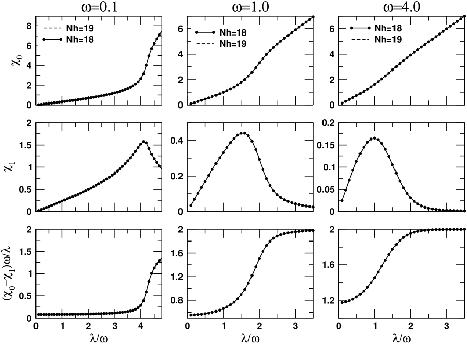
Figure 6: Figures in the upper row shows the $\chi$(0) at three different $\omega$. Middle row is for $\chi$(1). Lower row is for ($\chi$(0)-$\chi$(1))/g

5 The First Excited-State in an ordered Holstein model

In this section we discuss our calculation for the first excited state of the electron-phonon system. The first excited state consists of the ground state polaron and an unbounded extra phonon excitation[8]. Here the energy difference between the ground state and the first excited state should be equal to $\omega$ for a infinite chain(i.e., thermodynamic limit) and the mean phonon number difference should be equal to one(i.e., $\Delta N^{ph}$=1.0). But for the excited state there are two distinct regimes, one below the critical electron-phonon coupling $\lambda_{c}$ where the excited phonon tries to be at a infinite distance away from the ground state polaron(but the finite size of the system hinders it)and above it where the excited phonon is absorbed by the ground state polaron forming a bound state. The calculations here are done for $\omega$=0.5. VAED[8] calculations showed that a phase-transition occurs in the first excited state at $\lambda_{c}$=0.95(i.e., g=1.9) for $\omega$=0.5. Our calculations shows a phase-transition precisely at $\lambda$=0.95. Our calculated binding energy ( for the first excited state) and correlation functions clearly answers to the issue, whether the extra phonon excitation forms a bound state with the ground state polaron after a certain point(i,e., $\lambda_{c}$) or prefers to remain infinitely separated(of course limited by the finite size of the system) for all values of $\lambda$.

The binding energy $\Delta=\Delta E$ - $\omega$(where $\Delta E=E_{1}-E_{0}$, $E_{1}$ and $E_{0}$ are the first-excited-state and ground-state energy respectively) as a function of electron-phonon coupling $\lambda$ is shown in figure7 for various system sizes. Below $\lambda_{c}$, $\Delta$ varies with system size but is greater than zero. This variation with system size is due to the fact, that the excited phonon want to be infinitely away from the the ground state polaron, but the system size limits its ability. As the system size increases it slowly approaches the thermodynamic limit, i.e., $\Delta$=0. For $\lambda>\lambda_{c}$, where the absorption of the excited phonon by the ground-state-polaron has resulted in formation of a bound state, $\Delta$ has clearly converged at Nh=14 and is negative.

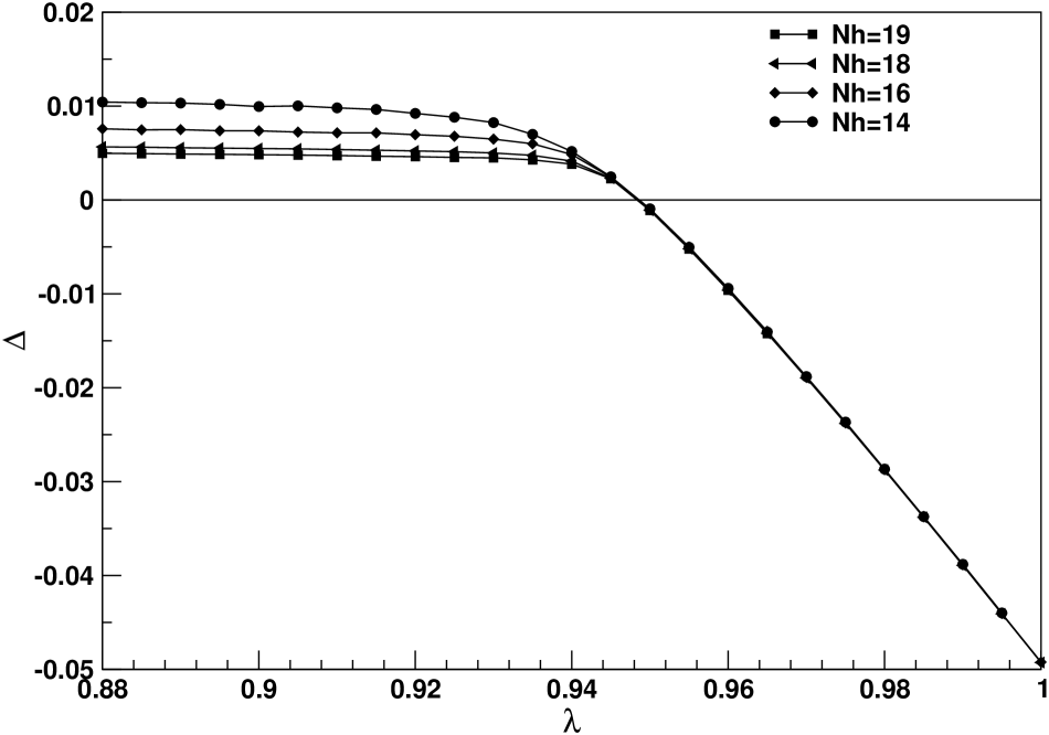
Figure 7: Figures shows the binding energy as a function of $\lambda$ for different system sizes(i.e., using different shell maps).

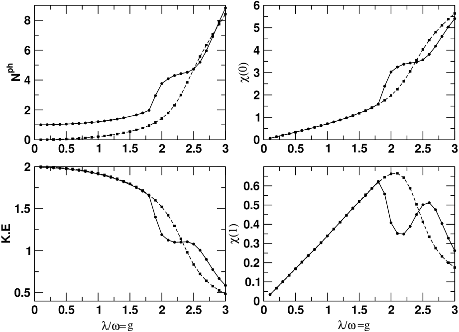
Figure 8: Figures show the comparison between the first excited state and ground state Correlation Functions at $\omega$=0.5. Phase transition in the first excited state occurs at $\gamma$=0.95 i.e., g=1.9. Solid line with dots are results for the first excited state and dashed line with squares are results for the ground state.

Figure8 compares the different correlation functions of the first excited state and the ground state for $\omega$=0.5. There is steady difference in between $N^{ph}$ of the first excited and the ground state($\Delta N^{ph}\simeq$1.0 ) below g=1.9, and then starts diverging. They again appears to converge at higher g though our excited state are not very accurate for higher g. Average kinetic energy, $\chi$(0), $\chi$(1) are same for the ground state and the excited state below $\lambda_{c}$ which very clearly indicates that below $\lambda_{c}$ the excited phonon and the ground state polaron are unbounded. The average kinetic energy, $\chi$(0), $\chi$(1) of the first excited state below $\lambda_{c}$ are entirely that of the ground state polaron and it is transparent to the presence of the excited phonon[8]. At $\lambda_{c}$ the root site disassociates itself from the rest of the lattice[8], the signature of which can be found in the sudden rise in $\chi$(0) and corresponding fall in $\chi$(1) . The bound state formed by the absorption of the excited phonon by the ground state polaron is a excited polaron. It slowly stabilizes with increasing $\lambda$ and exhibits the behavior of a de-excited polaron.

In figure 9 we have calculated the distribution of the number of excited phonons in the vicinity of the electron $\gamma(R_{i}-R_{j})$. We show $\gamma(R_{i}-R_{j})$ both for ground state ($\gamma_{0}$) and and excited state($\gamma_{1}$) just above($\lambda$=1.0) and below ($\lambda$=0.9) the transition point. Below the transition point the peaks of $\gamma_{0}$ and $\gamma_{1}$ are almost same , but $\gamma_{1}$ has a longer tail suggesting that tail represent the extra excited phonon which extends throughout the system in its attempt to remain unbounded from the ground state polaron. Our calculated $N_{ph}$ are same as VAED[8] for all the cases. The difference in between the ground state $N_{ph}$ and first excited state $N_{ph}$ should be one for a infinite system, but our difference is about 1.02 and this can be attributed to finite size effect[8]. The situation above $\lambda_{c}$ is different. Here the peak value of $\gamma_{1}$ is almost three times the peak value of $\gamma_{0}$ and secondly here $\gamma_{1}$ decays fast unlike that below $\lambda_{c}$. Here the difference in phonon number of the ground state and the excited state is 2.33 again exactly same as VAED[8]. Thus here the excited bound polaron has many extra phonon excitations compared to the ground state polaron. Since the extra phonon excitation are almost confined to the root site of the electron, it throws some light on the fact that at $\lambda_{c}$ the root site gets detached from the rest of the lattice[8].

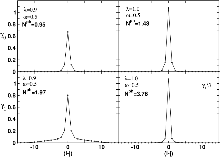
Figure 9: Figures shows the phonon number $\gamma$ as a function of the distance from the electron position $R_{i}-R_{j}$.

6 Results for a disordered Holstein model

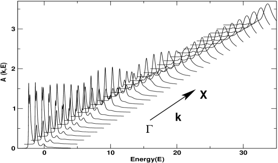
Figure 10: The spectral functions for the disordered Holstein model

Figure 11: Comparison of the average phonon number and kinetic energy for the disordered and ordered Holstein model at different oscillator frequencies

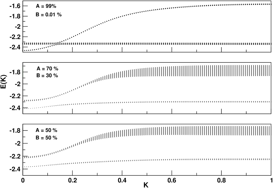
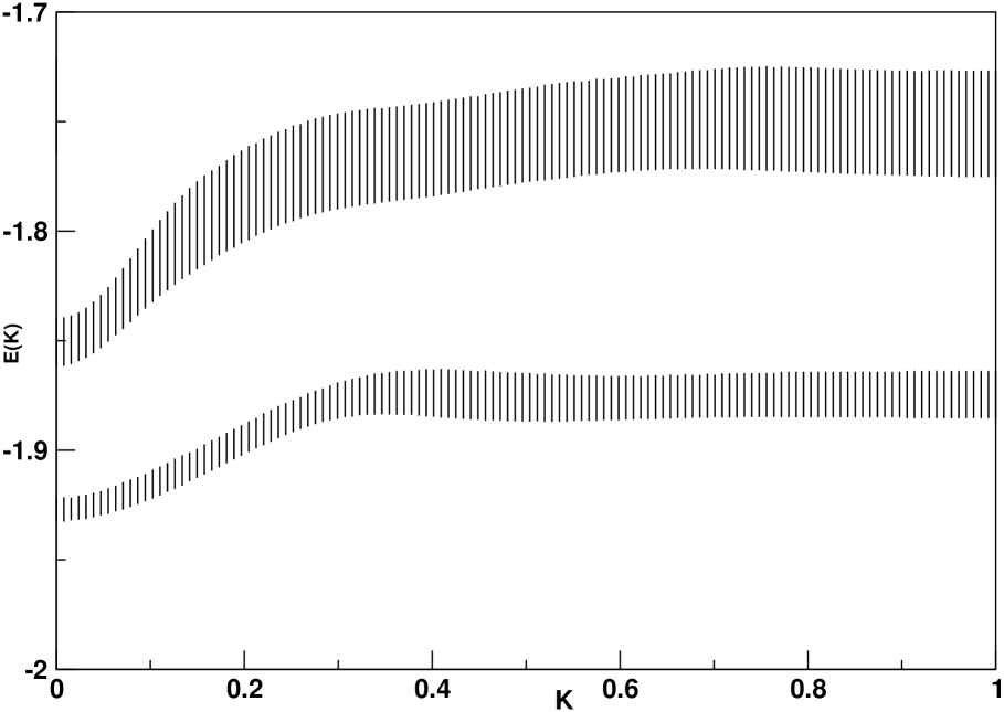
Figure 12: (Top) The dispersion curves for the disordered Holstein model, for g=1, $\epsilon_{A}$=0, $\epsilon_{B}$=0.5, for three different compositions. (Bottom) The dispersion curves for the disordered Holstein model, for g=0.01, $\epsilon_{A}$=0, $\epsilon_{B}$=0.5, for the 50-50 alloy.

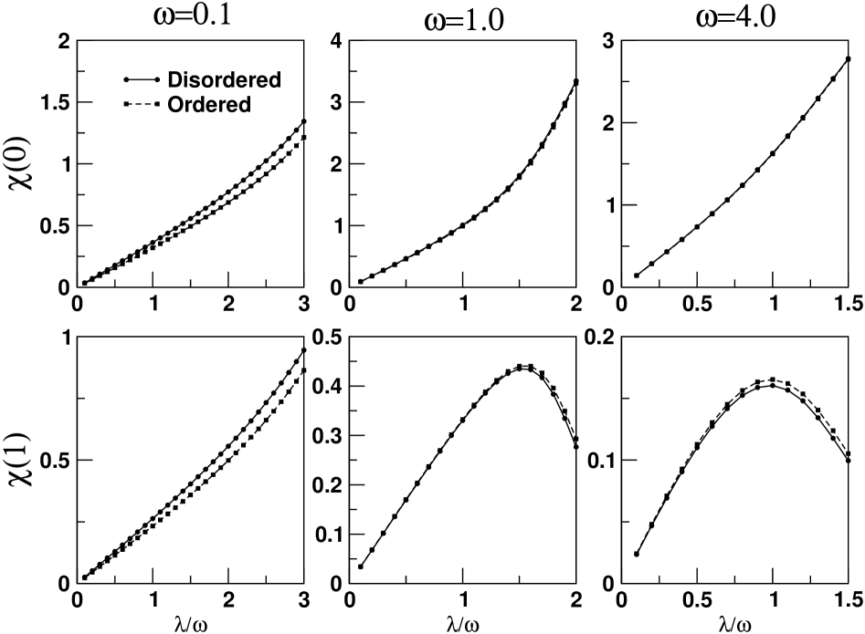
Figure 13: Comparison of $\chi$(0) and $\chi$(1) for the disordered and ordered Holstein model at different oscillator frequencies

In figure 10 we show the spectral function from the $\Gamma$ to $X$ point in Brillouin zone for the 50-50 alloy. The spectral functions show the extra disorder induced widths as well as contributions coming from both the components. This is much better seen in the dispersion curves shown in figure 12(top). The dispersion curves for both the disordered alloys show the two branches arising out of the two components and the large disorder induced widths in the upper band. In the low concentration impurity regime the two bands almost cross each other. For higher concentrations the bands are well separated. As in the ordered case, the lower band has very little width. In comparison with the ordered case the upper band has large width particularly near the Brillouin zone edge. This extra width arises from quenched disorder scattering. These dispersion curves are for g=1. Figure 12 (bottom) shows the

dispersion curves for g=0.01, i.e. low electron-phonon coupling. Here the disorder effect dominates and both the branches show disorder induced large smearing. For low electron-phonon coupling in a disordered alloy, the polaron, when formed, will have disorder scattering induced finite life-time. We conclude that disorder scattering effects are small on heavy polarons, while they tend to give larger lifetime effects to light polarons.

We have also calculated different ground state correlations functions for the disordered Holstein model and have compared it with its ordered counterparts to get a better insight of the disorder effect. Figure 11 compares the average phonon number and the average kinetic energy for the ordered and disordered case for three oscillator frequencies. Site disorder tends enhances the average phonon number with increasing electron-phonon coupling in the adiabatic regime where as, in the intermediate and anti-adiabatic regime disorder has hardly any effect. Disorder lowers the average kinetic energy in all the regimes. Figure 13 compares the $\chi$(0) and $\chi$(1) and similar trend is observed in this‘ set of correlation functions too. We conclude that the disordered effect is more prominent in the adiabatic regime and with increase in the oscillator frequency, the phononic disorder becomes dominant.

We would like to acknowledge effective discussions with Prof. A. N. Das and Dr. J. Chatterjee of SINP, Kolkata and Dr. P. A. Sreeram of SNBNCBS.

References

- [1] M. Jaime, H.T. Hardner, M.B. Salamon, M. Rubinstein, P. Dorsey and D. Emin, Phys. Rev. Lett. 78, 951(1997).
- [2] A.P. Ramirez, J. Phys.: Condens. Matter 9 , 8171,(1997)
- [3] I.H. Campbell and D.L. Smith, Solid State Phys.55,1 (2001).
- [4] Lattice Effects in High Superconductors, edited by Y. Baryam, T. Egami, J. Mustre de Leon, and A.R. Bishop (World Scientific,Singapore,1992)
- [5] A.S. Alexandrov and N.F. Mott,Rep. Prog. Phys. 57, 1197(1994)
- [6] T. Holstein, Ann. Phys. (NY) 8 325 (1959)
- [7] A.S. Alexandrov and N.F. Mott, Polarons and Bipolarons(world Scientific, Singapore,1995)
- [8] J. Bonca, S.A. Trugman, I. Batistic, Phys. Rev. B60 3, 1633(1999)
- [9] Li-Chung Ku, S.A. Trugman,J. Bonca, Phys. Rev. B65, 174306-1(2002)
- [10] F. X. Bronold, A. Saxena and A. R. Bishop, Phys. Rev. B 63, 235109(2001)
- [11] B. Sanyal, P.P. Biswas, M. Fakhruddin, A. Halder, M. Ahmed and A. Mookerjee, J. Phys. Condens Matter 7 8569-8575 (1995)
- [12] Eric Jeckelmann and Steven R. White, Phys. Rev. B 57,11,6376(1998)
- [13] A.S. Alexandrov, V.V. Kabanov and D.E. Ray, Phys. Rev. B 49, 9915(1994)
- [14] G. Wellien, H. Roder, and H. Fehske, Phys. Rev. B 53, 9666(1996)
- [15] G. Wellien and H. Fehske, Phys. Rev. B 56, 4513(1997)
- [16] G. Wellien and H. Fehske, Phys. Rev. B 58, 6802(1998)
- [17] E.V.L. de Mello and Ranninger, Phys. Rev. B 55,14, 872(1997)
- [18] M. Capone, W. Stephan and M. Grilli, Phys. Rev. B 56, 4484(1997)
- [19] F. Marsiglio, Physica C 244,21(1995)
- [20] H. De Raedt and A. Langedijk, Phys. Rev. Lett. 49, 1522(1982); Phys. Rev. B 27, 6097(1983); 30, 1671(1984)
- [21] P.E. Kornilovitch and E.R. Pike, Phys. Rev. BR8634,21(1997)
- [22] A.W. Romero, D.W. Brown and K. Lindenberg, J. Chem. Phys109,6540 (1998)
- [23] A.Mookerjee, J. Phys. Condens Matter 2 897 (1990)
- [24] R. Haydock, V. Heine and M.J. Kelly, J. Phys. C: Solid State Phys. 5 2845 (1972)
- [25] V.S. Viswanath and G. Müller, The user friendly recursion method : a cookbook for eclecticists, Troisieme Cycle de la Physique, En Suisse Romande (1993)
- [26] A function of a complex variable f(z) is called herglotz if : Im f(z) = -sgn[Im(z)] and f(z) as z along the real z line.
- [27] N. Beer and D.G. Pettifor, Electronic Structure of Complex Systems ed. P. Phariseau and W. M. Temmerman (Plenum, New York, 1984) p 769
- [28] A. Mookerjee, J. Phys. C: Solid State Phys. 6 L205 (1973).