Two-Hole Bound States from a Systematic
Low-Energy Effective Field Theory for
Magnons and Holes in an Antiferromagnet

Abstract

Identifying the correct low-energy effective theory for magnons and holes in an antiferromagnet has remained an open problem for a long time. In analogy to the effective theory for pions and nucleons in QCD, based on a symmetry analysis of Hubbard and $t$-$J$-type models, we construct a systematic low-energy effective field theory for magnons and holes located inside pockets centered at lattice momenta $(\pm\frac{\pi}{2a},\pm\frac{\pi}{2a})$. The effective theory is based on a nonlinear realization of the spontaneously broken spin symmetry and makes model-independent universal predictions for the entire class of lightly doped antiferromagnetic precursors of high-temperature superconductors. The predictions of the effective theory are exact, order by order in a systematic low-energy expansion. We derive the one-magnon exchange potentials between two holes in an otherwise undoped system. Remarkably, in some cases the corresponding two-hole Schrödinger equations can even be solved analytically. The resulting bound states have $d$-wave characteristics. The ground state wave function of two holes residing in different hole pockets has a $d_{x^{2}-y^{2}}$-like symmetry, while for two holes in the same pocket the symmetry resembles $d_{xy}$.

1 Introduction

The discovery of high-temperature superconductors [1] has motivated numerous studies of their doped antiferromagnetic precursors. In particular, the dynamics of holes in an antiferromagnet have been investigated in great detail in the condensed matter literature [2, 3, 4, 5, 6, 7, 8, 9, 10, 11, 12, 13, 14, 15, 16, 17, 18, 19, 20, 21, 22, 23, 24, 25, 26, 27, 28, 29, 30, 31, 32, 33, 34, 35, 36, 37, 38, 39, 40, 41, 42, 43]. However, a systematic investigation of these dynamics is complicated due to the strong correlations between the electrons in these systems. Unfortunately, away from half-filling, the standard microscopic Hubbard and $t$-$J$-type models cannot be solved numerically due to a severe fermion sign problem. Analytic calculations, on the other hand, usually suffer from uncontrolled approximations. Substantial progress has been made in the pioneering work of Chakravarty, Halperin, and Nelson [44] who described the low-energy magnon physics by an effective field theory — the $(2+1)$-d $O(3)$-invariant nonlinear $\sigma$-model. Based on this work, starting with Wen [11] and Shankar [13], there have been a number of approaches [21, 22, 27] that address the physics of both magnons and holes using effective field theories. All these approaches use composite vector fields to couple magnons and holes. The spin then appears as the “charge” of an Abelian gauge field. In this context, confinement of the spin “charge” and resulting spin-charge separation has sometimes been invoked. In these approaches an effective Lagrangian is usually obtained from an underlying microscopic system (e.g. from the Hubbard or $t$-$J$ model) by integrating out high-energy degrees of freedom. In this manner a variety of effective theories has been constructed. Unfortunately, there seems to be no agreement even on basic issues like the fermion field content of the effective theory or on the question how various symmetries are realized on those fields. In particular, it has never been demonstrated convincingly that any of the effective theories proposed so far indeed correctly describes the low-energy physics of the underlying microscopic systems quantitatively.

The experience with chiral perturbation theory for the strong interactions shows that effective field theory is able to provide a systematic — i.e. order by order exact — description of the low-energy physics of nonperturbative systems as complicated as QCD. One main goal of this paper is to provide the same for the antiferromagnetic precursors of high-temperature superconductors. Inspired by strongly interacting systems in particle physics [45, 46], we have recently approached the problem of constructing a low-energy effective field theory for magnons and holes in a systematic manner [47]. A central ingredient is the nonlinear realization of the spontaneously broken global symmetry [48, 49] — in this case of the $SU(2)_{s}$ spin symmetry. This again leads to the same composite vector fields that appeared in previous approaches to the problem. In particular, spin again appears as an Abelian “charge” to which a composite magnon “gauge” field couples. However, this gauge field does not mediate confining interactions. It just mediates magnon exchange, which represents a weak interaction at low energies. Consequently, spin-charge separation does not arise. In analogy to baryon chiral perturbation theory [50, 51, 52, 53, 54] — the effective theory for pions and nucleons — we have extended the pure magnon effective theory of [44, 55, 56, 57, 58, 59, 60, 61, 62, 63, 64] by including charge carriers. In [47] we have investigated the simplest case of charge carriers appearing at lattice momenta $(0,0)$ or $(\frac{\pi}{a},\frac{\pi}{a})$ in the Brillouin zone. However, angle resolved photoemission spectroscopy (ARPES) experiments [65, 66, 67, 68] as well as theoretical investigations [7, 6, 17, 39, 40] show that doped holes appear inside hole pockets centered at the lattice momenta $(\pm\frac{\pi}{2a},\pm\frac{\pi}{2a})$. In this paper, we generalize the effective theory of [47] to this case.

It should be pointed out that the effective theory to be constructed below is based on microscopic systems such as the Hubbard or $t$-$J$ model, but does not necessarily reflect all aspects of the actual cuprate materials. For example, just like the Hubbard or $t$-$J$ model, the effective theory does not contain impurities which are a necessary consequence of doping in the real materials. Also long-range Coulomb forces, anisotropies, or the effects of small couplings between different $CuO_{2}$ layers are neglected in the effective theory. Furthermore, the underlying crystal lattice is imposed as a rigid structure by hand, such that phonons are excluded from the outset. Although all these effects can in principle be incorporated in the effective theory, for the moment we exclude them, in order not to obscure the basic physics of magnons and holes. As a consequence, the effective theory does not describe the actual materials in all details. Still, it should be pointed out that the predictions of the effective theory are not limited to just the Hubbard or $t$-$J$ model, but are universally applicable to a wide range of microscopic systems. In fact, the low-energy physics of any antiferromagnet that possesses the assumed symmetries and has hole pockets at $(\pm\frac{\pi}{2a},\pm\frac{\pi}{2a})$ is described correctly, order by order in a systematic low-energy expansion. Material-specific properties enter the effective theory in the form of a priori undetermined low-energy parameters, such as the spin stiffness or the spinwave velocity. The values of the low-energy parameters for a concrete underlying microscopic system can be determined by comparison with experiments or with numerical simulations. For example, precise numerical simulations of low-energy observables in the $t$-$J$ model constitute a most stringent test of the effective theory. Such simulations are presently in progress.

After constructing the effective theory, we use it to calculate the one-magnon exchange potentials between two holes and we solve the corresponding Schrödinger equations. Remarkably, in some cases the Schrödinger equations can be solved completely analytically. The location of the hole pockets has an important effect on the dynamics and implies $d$-wave characteristics of hole pairs. Using the methods described in this paper, analogous to applications of baryon chiral perturbation theory to few-nucleon systems [69, 70, 71, 72, 73, 74, 75, 76, 77, 78], we have recently investigated magnon-mediated binding between two holes residing in two different hole pockets [79]. Here we discuss these issues in more detail and we extend the investigation to a pair of holes in the same pocket. In this paper, we limit ourselves to an isolated pair of holes in an otherwise undoped antiferromagnet. Lightly doped antiferromagnets will be investigated in a forthcoming publication [80].

The paper is organized as follows. In section 2 the symmetries of the microscopic Hubbard and $t$-$J$ models are summarized. Section 3 describes the nonlinear realization of the spontaneously broken $SU(2)_{s}$ spin symmetry. In section 4 the transformations of the effective fields for charge carriers are related to the ones of the underlying microscopic models. The hole fields are identified and the electron fields are eliminated in section 5. Also the leading terms in the effective Lagrangian for magnons and holes are constructed and accidental emergent flavor and Galilean boost symmetries are discussed. The resulting one-magnon exchange potentials are derived and the corresponding Schrödinger equations are studied in section 6. Finally, section 7 contains our conclusions.

2 Symmetries of Microscopic Models

The standard microscopic models for antiferromagnetism and high-temperature superconductivity are Hubbard and $t$-$J$-type models. The symmetries of these models are of central importance for the construction of the low-energy effective theories for magnons and charge carriers. The Hubbard model is defined by the Hamiltonian

$$H=-t\sum_{x,i}(c_{x}^{\dagger}c_{x+\hat{i}}+c_{x+\hat{i}}^{\dagger}c_{x})+\frac{U}{2}\sum_{x}(c_{x}^{\dagger}c_{x}-1)^{2}-\mu\sum_{x}(c_{x}^{\dagger}c_{x}-1).$$ (2.1)

Here $x$ denotes the sites of a 2-dimensional square lattice and $\hat{i}$ is a vector of length $a$ (where $a$ is the lattice spacing) pointing in the $i$-direction. Furthermore, $t$ is the nearest-neighbor hopping parameter, while $U>0$ is the strength of the screened on-site Coulomb repulsion, and $\mu$ is the chemical potential for fermion number relative to half-filling. The fermion creation and annihilation operators are given by

$$c_{x}^{\dagger}=(c_{x\uparrow}^{\dagger},c_{x\downarrow}^{\dagger}),\qquad c_{x}=\left(\begin{array}[]{c}c_{x\uparrow}\\ c_{x\downarrow}\end{array}\right).$$ (2.2)

They obey standard anticommutation relations. The $SU(2)_{s}$ symmetry is generated by the total spin

$$\vec{S}=\sum_{x}\vec{S}_{x}=\sum_{x}c_{x}^{\dagger}\ \frac{\vec{\sigma}}{2}\ c_{x},$$ (2.3)

where $\vec{\sigma}$ are the Pauli matrices, while the $U(1)_{Q}$ fermion number (relative to half-filling) is generated by the charge operator

$$Q=\sum_{x}Q_{x}=\sum_{x}(c_{x}^{\dagger}c_{x}-1)=\sum_{x}(c_{x\uparrow}^{\dagger}c_{x\uparrow}+c_{x\downarrow}^{\dagger}c_{x\downarrow}-1).$$ (2.4)

For $\mu=0$, the Hubbard model even possesses a non-Abelian $SU(2)_{Q}$ extension of the fermion number symmetry [81, 82] which is generated by

$$Q^{+}=\sum_{x}(-1)^{x}c_{x\uparrow}^{\dagger}c_{x\downarrow}^{\dagger},\quad Q^{-}=\sum_{x}(-1)^{x}c_{x\downarrow}c_{x\uparrow},\quad Q^{3}=\frac{1}{2}Q.$$ (2.5)

The factor $(-1)^{x}=(-1)^{(x_{1}+x_{2})/a}$ distinguishes between the sites of the even and odd sublattice. The points on the even sublattice have $(-1)^{x}=1$ while the points on the odd sublattice have $(-1)^{x}=-1$. As discussed in detail in [47], it is useful to introduce a matrix-valued fermion operator

$$C_{x}=\left(\begin{array}[]{cc}c_{x\uparrow}&(-1)^{x}\ c^{\dagger}_{x\downarrow}\\ c_{x\downarrow}&-(-1)^{x}c_{x\uparrow}^{\dagger}\end{array}\right),$$ (2.6)

which displays both the $SU(2)_{s}$ and the $SU(2)_{Q}$ symmetries in a compact form. Under combined transformations $g\in SU(2)_{s}$ and $\Omega\in SU(2)_{Q}$ it transforms as

$$^{\vec{Q}}C_{x}^{\prime}=gC_{x}\Omega^{T}.$$ (2.7)

Due to the antiferromagnetic order near half-filling, another important symmetry is the displacement $D_{i}$ by one lattice spacing in the $i$-direction which acts as

$${}^{D_{i}}C_{x}=C_{x+\hat{i}}\sigma_{3}.$$ (2.8)

The appearance of $\sigma_{3}$ on the right is due to the factor $(-1)^{x}$. As discussed in [47], it is also useful to introduce a combination $D^{\prime}_{i}$ of the displacement symmetry $D_{i}$ with the $SU(2)_{s}$ transformation $g=i\sigma_{2}$

$${}^{D^{\prime}_{i}}C_{x}=(i\sigma_{2})C_{x+\hat{i}}\sigma_{3}.$$ (2.9)

The Hamiltonian can then be expressed in the manifestly $SU(2)_{s}$-, $SU(2)_{Q}$-, $D_{i}$-, and thus also $D^{\prime}_{i}$-invariant form

$$H=-\frac{t}{2}\sum_{x,i}\mbox{Tr}[C_{x}^{\dagger}C_{x+\hat{i}}+C_{x+\hat{i}}^{\dagger}C_{x}]+\frac{U}{12}\sum_{x}\mbox{Tr}[C_{x}^{\dagger}C_{x}C_{x}^{\dagger}C_{x}]-\frac{\mu}{2}\sum_{x}\mbox{Tr}[C_{x}^{\dagger}C_{x}\sigma_{3}].$$ (2.10)

The chemical potential term is only $U(1)_{Q}$-invariant, while the other two terms are manifestly $SU(2)_{Q}$-invariant.

We also need to consider the 90 degrees rotation $O$ of the quadratic lattice. It acts on a point $x=(x_{1},x_{2})$ as $Ox=(-x_{2},x_{1})$. Under this symmetry the fermion operator matrix transforms as

$${}^{O}C_{x}=C_{Ox}.$$ (2.11)

Under the spatial reflection $R$ at the $x_{1}$-axis, which turns $x$ into $Rx=(x_{1},-x_{2})$, one obtains

$${}^{R}C_{x}=C_{Rx}.$$ (2.12)

It should be noted that, due to the presence of the lattice, the Hubbard model is not invariant under Galilean boosts.

The $t$-$J$ model is defined by the Hamilton operator

$$H=P\bigg{\{}-t\sum_{x,i}(c_{x}^{\dagger}c_{x+\hat{i}}+c_{x+\hat{i}}^{\dagger}c_{x})+J\sum_{x,i}\vec{S}_{x}\cdot\vec{S}_{x+\hat{i}}-\mu\sum_{x}Q_{x}\bigg{\}}P.$$ (2.13)

Now the operators act in a restricted Hilbert space of empty or at most singly occupied sites, while states with doubly occupied sites are eliminated from the Hilbert space by the projection operator $P$. Hence, the $t$-$J$ model can only be doped with holes but not with electrons. The $t$-$J$ model has the same symmetries as the Hubbard model, except that the $SU(2)_{Q}$ extension of the $U(1)_{Q}$ fermion number symmetry, which relates electrons to holes in the Hubbard model, is now absent.

In the $t$-$J$ model, a single hole has been simulated rather accurately in [39, 40]. Using a worm-cluster algorithm similar to the algorithm used in [40], we have computed the single-hole dispersion relation shown in figure 1. The energy $E(\vec{p})$ of a hole is minimal when its lattice momentum $\vec{p}=(p_{1},p_{2})$ is located in a hole pocket centered at $(\pm\frac{\pi}{2a},\pm\frac{\pi}{2a})$.

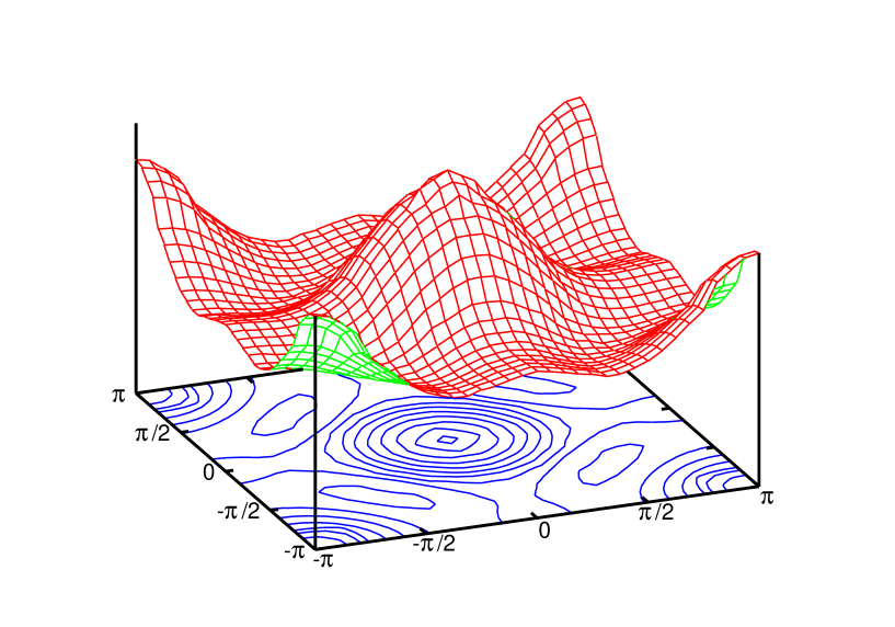
Figure 1: The dispersion relation $E(\vec{p})$ of a single hole in the $t$-$J$ model (on a $32\times 32$ lattice for $J=2t$) with hole pockets centered at $(\pm\frac{\pi}{2a},\pm\frac{\pi}{2a})$.

3 Nonlinear Realization of the $SU(2)_{s}$ Symmetry

The key to the low-energy physics of lightly doped cuprates is the spontaneous breakdown of the $SU(2)_{s}$ symmetry down to $U(1)_{s}$ which gives rise to two massless Nambu-Goldstone bosons — the antiferromagnetic magnons. Analogous to chiral perturbation theory for the Nambu-Goldstone pions in QCD [46], a systematic low-energy effective theory for magnons has been developed in [55, 56, 57, 58, 59, 61, 62, 60, 63]. In order to couple charge carriers to the magnons, a nonlinear realization of the $SU(2)_{s}$ symmetry has been constructed in [47]. The global $SU(2)_{s}$ symmetry then manifests itself as a local $U(1)_{s}$ symmetry in the unbroken subgroup. This is analogous to baryon chiral perturbation theory in which the spontaneously broken $SU(2)_{L}\otimes SU(2)_{R}$ chiral symmetry of QCD is implemented on the nucleon fields as a local $SU(2)_{L=R}$ transformation in the unbroken isospin subgroup.

The staggered magnetization of an antiferromagnet is described by a unit-vector field

$$\vec{e}(x)=(e_{1}(x),e_{2}(x),e_{3}(x)),\qquad\vec{e}(x)^{2}=1,$$ (3.1)

in the coset space $SU(2)_{s}/U(1)_{s}=S^{2}$. Here $x=(x_{1},x_{2},t)$ denotes a point in space-time. An equivalent $CP(1)$ representation uses $2\times 2$ Hermitean projection matrices $P(x)$ that obey

$$P(x)=\frac{1}{2}({\mathbbm{1}}+\vec{e}(x)\cdot\vec{\sigma}),\quad P(x)^{\dagger}=P(x),\quad\mbox{Tr}P(x)=1,\quad P(x)^{2}=P(x).$$ (3.2)

To leading order, the Euclidean magnon effective action takes the form

$$S[P]=\int d^{2}x\ dt\ \rho_{s}\mbox{Tr}\Big{[}\partial_{i}P\partial_{i}P+\frac{1}{c^{2}}\partial_{t}P\partial_{t}P\Big{]}.$$ (3.3)

The index $i\in\{1,2\}$ labels the two spatial directions, while the index $t$ refers to the time-direction. The parameter $\rho_{s}$ is the spin stiffness and $c$ is the spinwave velocity. As discussed in detail in [47], the action is invariant under the symmetries of the corresponding microscopic models which are realized as follows in the effective theory

$$SU(2)_{s}: P(x)^{\prime} =gP(x)g^{\dagger},$$

$$SU(2)_{Q}: {}^{\vec{Q}}P(x) =P(x),$$

$$D_{i}: {}^{D_{i}}P(x) ={\mathbbm{1}}-P(x),$$

$$D^{\prime}_{i}: {}^{D^{\prime}_{i}}P(x) =P(x)^{*},$$

$$O: {}^{O}P(x) =P(Ox), \quad Ox =(-x_{2},x_{1},t),$$

$$R: {}^{R}P(x) =P(Rx), \quad Rx =(x_{1},-x_{2},t),$$

$$T: {}^{T}P(x) ={\mathbbm{1}}-P(Tx), \quad Tx =(x_{1},x_{2},-t),$$

$$T^{\prime}: {}^{T^{\prime}}P(x) =(i\sigma_{2})\;\left[{}^{T}P(x)\right](i\sigma_{2})^{\dagger}=P(Tx)^{*}.$$ (3.4)

Here $T$ denotes time-reversal. The symmetry $T^{\prime}$ combines $T$ with the $SU(2)_{s}$ rotation $g=i\sigma_{2}$.

The definition of the nonlinear realization of the $SU(2)_{s}$ symmetry proceeds as follows. First, one diagonalizes the magnon field by a unitary transformation $u(x)\in SU(2)$, i.e.

$$u(x)P(x)u(x)^{\dagger}=\frac{1}{2}({\mathbbm{1}}+\sigma_{3})=\left(\begin{array}[]{cc}1&0\\ 0&0\end{array}\right),\qquad u_{11}(x)\geq 0.$$ (3.5)

Parameterizing

$$\vec{e}(x)=(\sin\theta(x)\cos\varphi(x),\sin\theta(x)\sin\varphi(x),\cos\theta(x)),$$ (3.6)

one obtains

$$u(x)=\left(\begin{array}[]{cc}\cos(\frac{1}{2}\theta(x))&\sin(\frac{1}{2}\theta(x))\exp(-i\varphi(x))\\ -\sin(\frac{1}{2}\theta(x))\exp(i\varphi(x))&\cos(\frac{1}{2}\theta(x))\end{array}\right).$$ (3.7)

Under a global $SU(2)_{s}$ transformation $g$, the diagonalizing field $u(x)$ transforms as

$$u(x)^{\prime}=h(x)u(x)g^{\dagger},\qquad u_{11}(x)^{\prime}\geq 0,$$ (3.8)

which implicitly defines the nonlinear symmetry transformation

$$h(x)=\exp(i\alpha(x)\sigma_{3})=\left(\begin{array}[]{cc}\exp(i\alpha(x))&0\\ 0&\exp(-i\alpha(x))\end{array}\right)\in U(1)_{s}.$$ (3.9)

Under the displacement symmetry $D_{i}$ the staggered magnetization changes sign, i.e. ${}^{D_{i}}\vec{e}(x)=-\vec{e}(x)$, such that one obtains

$${}^{D_{i}}u(x)=\tau(x)u(x),$$ (3.10)

with

$$\tau(x)=\left(\begin{array}[]{cc}0&-\exp(-i\varphi(x))\\ \exp(i\varphi(x))&0\end{array}\right).$$ (3.11)

Introducing the traceless anti-Hermitean field

$$v_{\mu}(x)=u(x)\partial_{\mu}u(x)^{\dagger},$$ (3.12)

one obtains the following transformation rules

$$SU(2)_{s}: v_{\mu}(x)^{\prime} =h(x)[v_{\mu}(x)+\partial_{\mu}]h(x)^{\dagger},$$

$$SU(2)_{Q}: {}^{\vec{Q}}v_{\mu}(x) =v_{\mu}(x),$$

$$D_{i}: {}^{D_{i}}v_{\mu}(x) =\tau(x)[v_{\mu}(x)+\partial_{\mu}]\tau(x)^{\dagger},$$

$$D^{\prime}_{i}: {}^{D^{\prime}_{i}}v_{\mu}(x) =v_{\mu}(x)^{*},$$

$$O: {}^{O}v_{i}(x) =\varepsilon_{ij}v_{j}(Ox),\quad {}^{O}v_{t}(x) =v_{t}(Ox),$$

$$R: {}^{R}v_{1}(x) =v_{1}(Rx),\quad {}^{R}v_{2}(x) =-v_{2}(Rx),\quad^{R}v_{t}(x)=v_{t}(Rx),$$

$$T: {}^{T}v_{j}(x) =\ ^{D_{i}}v_{j}(Tx),\quad {}^{T}v_{t}(x) =-\ ^{D_{i}}v_{t}(Tx),$$

$$T^{\prime}: {}^{T^{\prime}}v_{j}(x) =\ ^{D^{\prime}_{i}}v_{j}(Tx),\quad {}^{T^{\prime}}v_{t}(x) =-^{D^{\prime}_{i}}v_{t}(Tx).$$ (3.13)

Writing

$$v_{\mu}(x)=iv_{\mu}^{a}(x)\sigma_{a},\qquad v_{\mu}^{\pm}(x)=v_{\mu}^{1}(x)\mp iv_{\mu}^{2}(x),$$ (3.14)

the field $v_{\mu}(x)$ decomposes into an Abelian “gauge” field $v_{\mu}^{3}(x)$ and two “charged” vector fields $v_{\mu}^{\pm}(x)$.

4 Transformation Rules of Charge Carrier Fields

Due to the nonperturbative dynamics, it is impossible in practice to rigorously derive the low-energy effective theory from the underlying microscopic physics. Still, in this section we will attempt to relate the transformation rules of the effective fields describing the charge carriers to those of the microscopic fermion operator matrix $C_{x}$ of eq.(2.6).

4.1 Sublattice Fermion Fields

In [47] we have introduced operators $\Psi^{A}_{x}$ and $\Psi^{B}_{x}$ on the even and odd sublattices $\Psi^{A,B}_{x}=u(x)C_{x}$ with $(-1)^{x}=1$ for $A$ and $(-1)^{x}=-1$ for $B$. In the Brillouin zone the corresponding linear combinations $\Psi^{A}_{x}\pm\Psi^{B}_{x}$ are located at lattice momenta $(0,0)$ and $(\frac{\pi}{a},\frac{\pi}{a})$. In order to account for the experimentally observed [65, 66, 67, 68] as well as theoretically predicted [7, 6, 17, 39, 40] hole pockets centered at $(\pm\frac{\pi}{2a},\pm\frac{\pi}{2a})$, we now introduce eight sublattices $A$, $B$, …, $H$ as illustrated in figure 2.

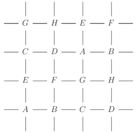
Figure 2: The layout of the eight sublattices $A$, $B$, …, $H$.

While it would be unnatural to introduce more than two sublattices in a pure antiferromagnet, the eight sublattices are a natural and even necessary concept when one wants to describe fermions located in hole pockets centered at $(\pm\frac{\pi}{2a},\pm\frac{\pi}{2a})$. We now introduce new lattice operators

$$\Psi^{A,B,...,H}_{x}=u(x)C_{x},\qquad x\in A,B,...,H,$$ (4.1)

which inherit their transformation properties from the operators of the Hubbard model. According to eqs.(3.8) and (2.7), under the $SU(2)_{s}$ symmetry one obtains

$${\Psi_{x}^{X}}^{\prime}=u(x)^{\prime}C_{x}^{\prime}=h(x)u(x)g^{\dagger}gC_{x}=h(x)\Psi_{x}^{X},\qquad X\in\{A,B,...,H\}.$$ (4.2)

Similarly, under the $SU(2)_{Q}$ symmetry one obtains

$${}^{\vec{Q}}\Psi_{x}^{X}={}^{\vec{Q}}u(x)^{\vec{Q}}C_{x}=u(x)C_{x}\Omega^{T}=\Psi_{x}^{X}\Omega^{T}.$$ (4.3)

Under the displacement symmetry the new operators transform as

$${}^{D_{i}}\Psi^{X}_{x}={}^{D_{i}}u(x+\hat{i})C_{x+\hat{i}}\sigma_{3}=\tau(x+\hat{i})u(x+\hat{i})C_{x+\hat{i}}\sigma_{3}=\tau(x+\hat{i})\Psi^{D_{i}X}_{x+\hat{i}}\sigma_{3},$$ (4.4)

where $\tau(x)$ is the field introduced in eq.(3.11) and $D_{i}X$ is the sublattice that one obtains by shifting sublattice $X$ by one lattice spacing in the $i$-direction. Similarly, under the symmetry $D^{\prime}_{i}$ one finds

$${}^{D^{\prime}_{i}}\Psi^{X}_{x}={}^{D^{\prime}_{i}}u(x+\hat{i})(i\sigma_{2})C_{x+\hat{i}}\sigma_{3}=u(x+\hat{i})^{*}(i\sigma_{2})C_{x+\hat{i}}\sigma_{3}=(i\sigma_{2})\Psi^{D_{i}X}_{x+\hat{i}}\sigma_{3},$$ (4.5)

while under the 90 degrees rotation $O$

$${}^{O}\Psi^{X}_{x}={}^{O}u(x)\,^{O}C_{x}=u(Ox)C_{Ox}=\Psi^{OX}_{Ox},$$ (4.6)

and under the reflection $R$

$${}^{R}\Psi^{X}_{x}={}^{R}u(x)\,^{R}C_{x}=u(Rx)C_{Rx}=\Psi^{RX}_{Rx}.$$ (4.7)

Here $OX$ and $RX$ are the sublattices obtained by rotating or reflecting the sublattice $X$. We arbitrarily chose the origin to lie on sublattice $A$.

In the low-energy effective theory we will use a path integral description instead of the Hamiltonian description used in the Hubbard model. In the effective theory the electron and hole fields are thus represented by independent Grassmann numbers $\psi^{A,B,...,H}_{\pm}(x)$ and $\psi^{A,B,...,H\dagger}_{\pm}(x)$ which are combined to

$$\Psi^{X}(x)=\left(\begin{array}[]{cc}\psi^{X}_{+}(x)&\psi^{X\dagger}_{-}(x)\\ \psi^{X}_{-}(x)&-\psi^{X\dagger}_{+}(x)\end{array}\right),\qquad X\in\{A,C,F,H\},$$ (4.10)

$$\Psi^{X}(x)=\left(\begin{array}[]{cc}\psi^{X}_{+}(x)&-\psi^{X\dagger}_{-}(x)\\ \psi^{X}_{-}(x)&\psi^{X\dagger}_{+}(x)\end{array}\right),\qquad X\in\{B,D,E,G\}.$$ (4.13)

Note that the even sublattices $A,C,F,H$ (with $(-1)^{x}=1$) are treated differently than the odd sublattices $B,D,E,G$ (with $(-1)^{x}=-1$). For notational convenience, we also introduce the fields

$$\Psi^{X\dagger}(x)=\left(\begin{array}[]{cc}\psi^{X\dagger}_{+}(x)&\psi^{X\dagger}_{-}(x)\\ \psi^{X}_{-}(x)&-\psi^{X}_{+}(x)\end{array}\right),\qquad X\in\{A,C,F,H\},$$ (4.16)

$$\Psi^{X\dagger}(x)=\left(\begin{array}[]{cc}\psi^{X\dagger}_{+}(x)&\psi^{X\dagger}_{-}(x)\\ -\psi^{X}_{-}(x)&\psi^{X}_{+}(x)\end{array}\right),\qquad X\in\{B,D,E,G\},$$ (4.19)

which consist of the same Grassmann fields $\psi^{X}_{\pm}(x)$ and $\psi^{X\dagger}_{\pm}(x)$ as $\Psi^{X}(x)$.

In contrast to the lattice operators, the fields $\Psi^{X}(x)$ are defined in the continuum. Hence, under the displacement symmetries $D_{i}$ and $D^{\prime}_{i}$ we no longer distinguish between the points $x$ and $x+\hat{i}$. As a result, the transformation rules of the various symmetries take the form

$$SU(2)_{s}: \Psi^{X}(x)^{\prime} =h(x)\Psi^{X}(x),$$

$$SU(2)_{Q}: {}^{\vec{Q}}\Psi^{X}(x) =\Psi^{X}(x)\Omega^{T},$$

$$D_{i}: {}^{D_{i}}\Psi^{X}(x) =\tau(x)\Psi^{D_{i}X}(x)\sigma_{3},$$

$$D^{\prime}_{i}: {}^{D^{\prime}_{i}}\Psi^{X}(x) =(i\sigma_{2})\Psi^{D_{i}X}(x)\sigma_{3},$$

$$O: {}^{O}\Psi^{X}(x) =\Psi^{OX}(Ox),$$

$$R: {}^{R}\Psi^{X}(x) =\Psi^{RX}(Rx),$$

$$T: {}^{T}\Psi^{X}(x) =\tau(Tx)(i\sigma_{2})\left[\Psi^{X\dagger}(Tx)^{T}\right]\sigma_{3},$$

$${}^{T}\Psi^{X\dagger}(x) =-\sigma_{3}\left[\Psi^{X}(Tx)^{T}\right](i\sigma_{2})^{\dagger}\tau(Tx)^{\dagger},$$

$$T^{\prime}: {}^{T^{\prime}}\Psi^{X}(x) =-\left[\Psi^{X\dagger}(Tx)^{T}\right]\sigma_{3},$$

$${}^{T^{\prime}}\Psi^{X\dagger}(x) =\sigma_{3}\left[\Psi^{X}(Tx)^{T}\right].$$ (4.20)

Note that an upper index $T$ on the right denotes transpose, while on the left it denotes time-reversal. The form of the time-reversal symmetry $T$ in the effective theory with nonlinearly realized $SU(2)_{s}$ symmetry follows from the usual form of time-reversal in the path integral of a nonrelativistic theory in which the spin symmetry is linearly realized. The fermion fields in the two formulations just differ by a factor $u(x)$. In components the transformation rules take the form

$$SU(2)_{s}: \psi^{X}_{\pm}(x)^{\prime} =\exp(\pm i\alpha(x))\psi^{X}_{\pm}(x),$$

$$U(1)_{Q}: {}^{Q}\psi^{X}_{\pm}(x) =\exp(i\omega)\psi^{X}_{\pm}(x),$$

$$D_{i}: {}^{D_{i}}\psi^{X}_{\pm}(x) =\mp\exp(\mp i\varphi(x))\psi^{D_{i}X}_{\mp}(x),$$

$$D^{\prime}_{i}: {}^{D^{\prime}_{i}}\psi^{X}_{\pm}(x) =\pm\psi^{D_{i}X}_{\mp}(x),$$

$$O: {}^{O}\psi^{X}_{\pm}(x) =\psi^{OX}_{\pm}(Ox),$$

$$R: {}^{R}\psi^{X}_{\pm}(x) =\psi^{RX}_{\pm}(Rx),$$

$$T: {}^{T}\psi^{X}_{\pm}(x) =\exp(\mp i\varphi(Tx))\psi^{X\dagger}_{\pm}(Tx),$$

$${}^{T}\psi^{X\dagger}_{\pm}(x) =-\exp(\pm i\varphi(Tx))\psi^{X}_{\pm}(Tx),$$

$$T^{\prime}: {}^{T^{\prime}}\psi^{X}_{\pm}(x) =-\psi^{X\dagger}_{\pm}(Tx),$$

$${}^{T^{\prime}}\psi^{X\dagger}_{\pm}(x) =\psi^{X}_{\pm}(Tx).$$ (4.21)

4.2 Fermion Fields in Momentum Space Pockets

Instead of working with the eight sublattice indices $X\in\{A,B,...,H\}$, it is more convenient to introduce eight corresponding lattice momentum indices

$$k=(k_{1},k_{2})\in\left\{\big{(}0,0\big{)},\;\big{(}\frac{\pi}{a},\frac{\pi}{a}\big{)},\;\big{(}\frac{\pi}{a},0\big{)},\;\big{(}0,\frac{\pi}{a}\big{)},\;\big{(}\pm\frac{\pi}{2a},\pm\frac{\pi}{2a}\big{)}\right\}.$$ (4.22)

The eight sublattices represent a minimal set that allows us to address the lattice momenta $(\pm\frac{\pi}{2a},\pm\frac{\pi}{2a})$ which define the centers of hole pockets in the cuprates. By introducing further sublattices it would be straightforward to reach other lattice momenta as well. With the present construction we restrict ourselves to the momenta listed above and illustrated in figure 3.

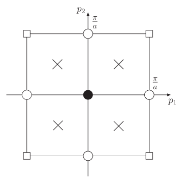
Figure 3: The eight lattice momenta (and their periodic copies) dual to the eight sublattices $A$, $B$,…,$H$. In the cuprates the holes reside in momentum space pockets centered at lattice momenta $\big{(}\pm\frac{\pi}{2a},\pm\frac{\pi}{2a}\big{)}$ which are represented by the four crosses.

We now construct new fields

$$\psi^{k}_{\pm}(x)= \;\frac{1}{\sqrt{8}}\Big{\{}\psi^{A}_{\pm}(x)+e^{-ik_{1}a}\psi^{B}_{\pm}(x)+e^{-2ik_{1}a}\psi^{C}_{\pm}(x)+e^{-3ik_{1}a}\psi^{D}_{\pm}(x)$$

$$+e^{-ik_{2}a}[\psi^{E}_{\pm}(x)+e^{-ik_{1}a}\psi^{F}_{\pm}(x)+e^{-2ik_{1}a}\psi^{G}_{\pm}(x)+e^{-3ik_{1}a}\psi^{H}_{\pm}(x)]\Big{\}},$$ (4.23)

which transform as

$$SU(2)_{s}: \psi^{k}_{\pm}(x)^{\prime} =\exp(\pm i\alpha(x))\psi^{k}_{\pm}(x),$$

$$U(1)_{Q}: {}^{Q}\psi^{k}_{\pm}(x) =\exp(i\omega)\psi^{k}_{\pm}(x),$$

$$D_{i}: {}^{D_{i}}\psi^{k}_{\pm}(x) =\mp\exp(ik_{i}a)\exp(\mp i\varphi(x))\psi^{k}_{\mp}(x),$$

$$D^{\prime}_{i}: {}^{D^{\prime}_{i}}\psi^{k}_{\pm}(x) =\pm\exp(ik_{i}a)\psi^{k}_{\mp}(x),$$

$$O: {}^{O}\psi^{k}_{\pm}(x) =\psi^{Ok}_{\pm}(Ox),$$

$$R: {}^{R}\psi^{k}_{\pm}(x) =\psi^{Rk}_{\pm}(Rx),$$

$$T: {}^{T}\psi^{k}_{\pm}(x) =\exp(\mp i\varphi(Tx))\psi^{-k\dagger}_{\pm}(Tx),$$

$${}^{T}\psi^{k\dagger}_{\pm}(x) =-\exp(\pm i\varphi(Tx))\psi^{-k}_{\pm}(Tx),$$

$$T^{\prime}: {}^{T^{\prime}}\psi^{k}_{\pm}(x) =-\psi^{-k\dagger}_{\pm}(Tx),$$

$${}^{T^{\prime}}\psi^{k\dagger}_{\pm}(x) =\psi^{-k}_{\pm}(Tx).$$ (4.24)

Here $Ok$ and $Rk$ are the momenta obtained by rotating or reflecting the lattice momentum $k$. From the component fields one can again construct matrix-valued fields

$$\Psi^{k}(x)=\left(\begin{array}[]{cc}\psi^{k}_{+}(x)&\psi^{-k^{\prime}\dagger}_{-}(x)\\ \psi^{k}_{-}(x)&-\psi^{-k^{\prime}\dagger}_{+}(x)\end{array}\right),\quad\Psi^{k\dagger}(x)=\left(\begin{array}[]{cc}\psi^{k\dagger}_{+}(x)&\psi^{k\dagger}_{-}(x)\\ \psi^{-k^{\prime}}_{-}(x)&-\psi^{-k^{\prime}}_{+}(x)\end{array}\right),$$ (4.25)

with $k^{\prime}=k+(\frac{\pi}{a},\frac{\pi}{a})$. The matrix-valued fields then transform as

$$SU(2)_{s}: \Psi^{k}(x)^{\prime} =h(x)\Psi^{k}(x),$$

$$SU(2)_{Q}: {}^{\vec{Q}}\Psi^{k}(x) =\Psi^{k}(x)\Omega^{T},$$

$$D_{i}: {}^{D_{i}}\Psi^{k}(x) =\exp(ik_{i}a)\tau(x)\Psi^{k}(x)\sigma_{3},$$

$$D^{\prime}_{i}: {}^{D^{\prime}_{i}}\Psi^{k}(x) =\exp(ik_{i}a)(i\sigma_{2})\Psi^{k}(x)\sigma_{3},$$

$$O: {}^{O}\Psi^{k}(x) =\Psi^{Ok}(Ox),$$

$$R: {}^{R}\Psi^{k}(x) =\Psi^{Rk}(Rx),$$

$$T: {}^{T}\Psi^{k}(x) =\tau(Tx)(i\sigma_{2})\left[\Psi^{-k\dagger}(Tx)^{T}\right]\sigma_{3},$$

$${}^{T}\Psi^{k\dagger}(x) =-\sigma_{3}\left[\Psi^{-k}(Tx)^{T}\right](i\sigma_{2})^{\dagger}\tau(Tx)^{\dagger},$$

$$T^{\prime}: {}^{T^{\prime}}\Psi^{k}(x) =-\left[\Psi^{-k\dagger}(Tx)^{T}\right]\sigma_{3},$$

$${}^{T^{\prime}}\Psi^{k\dagger}(x) =\sigma_{3}\left[\Psi^{-k}(Tx)^{T}\right].$$ (4.26)

In [47] we have limited ourselves to two sublattices $A$ and $B$ which leads to the lattice momenta $(0,0)$ and $(\frac{\pi}{a},\frac{\pi}{a})$. The main purpose of the present paper is to describe holes located in pockets centered at $(\pm\frac{\pi}{2a},\pm\frac{\pi}{2a})$.

5 Effective Theory for Magnons and Holes

From now on we will limit ourselves to theories with holes as the only charge carriers. In order to identify the hole and to eliminate the electron fields, we consider the most general mass terms consistent with the symmetries.

5.1 Hole Field Identification and Electron Field Elimination

It turns out that mass terms cannot mix the various lattice momenta arbitrarily. In particular, through a mass term a field $\psi^{k}_{\pm}(x)$ with lattice momentum $k$ can only mix with fields with lattice momenta $k$ or $k^{\prime}$. Hence, the eight lattice momenta can be divided into four pairs which are associated with three different cases. The simplest case in which $k=(0,0)$ and $k^{\prime}=(\frac{\pi}{a},\frac{\pi}{a})$ has been investigated in great detail in [47], but is not realized in the cuprates. Another case in which $k=(\frac{\pi}{a},0)$ and $k^{\prime}=(0,\frac{\pi}{a})$ describes electron doping and will be investigated elsewhere. In the following, we concentrate on hole-doped cuprates. In this case, the hole pockets are centered at lattice momenta

$$k^{\alpha}=\big{(}\frac{\pi}{2a},\,\frac{\pi}{2a}\big{)},\quad{k^{\alpha}}^{\prime}=-k^{\alpha},\qquad k^{\beta}=\big{(}\frac{\pi}{2a},-\frac{\pi}{2a}\big{)},\quad{k^{\beta}}^{\prime}=-k^{\beta}.$$ (5.1)

Using the transformation rules of eq.(4.2) one can construct the following invariant mass terms

$$\sum_{f=\alpha,\beta} \frac{1}{2}\mbox{Tr}\big{[}{\cal M}(\Psi^{k^{f}\dagger}\sigma_{3}\Psi^{{k^{f}}^{\prime}}+\Psi^{{k^{f}}^{\prime}\dagger}\sigma_{3}\Psi^{k^{f}})+m(\Psi^{k^{f}\dagger}\Psi^{k^{f}}\sigma_{3}+\Psi^{{k^{f}}^{\prime}\dagger}\Psi^{{k^{f}}^{\prime}}\sigma_{3})\big{]}$$

$$= \,\sum_{f=\alpha,\beta}\big{[}{\cal M}\big{(}\psi^{k^{f}\dagger}_{+}\psi^{{k^{f}}^{\prime}}_{+}-\psi^{k^{f}\dagger}_{-}\psi^{{k^{f}}^{\prime}}_{-}+\psi^{{k^{f}}^{\prime}\dagger}_{+}\psi^{k^{f}}_{+}-\psi^{{k^{f}}^{\prime}\dagger}_{-}\psi^{k^{f}}_{-}\big{)}$$

$$\,\hskip 25.00003pt+m\big{(}\psi^{k^{f}\dagger}_{+}\psi^{k^{f}}_{+}+\psi^{k^{f}\dagger}_{-}\psi^{k^{f}}_{-}+\psi^{{k^{f}}^{\prime}\dagger}_{+}\psi^{{k^{f}}^{\prime}}_{+}+\psi^{{k^{f}}^{\prime}\dagger}_{-}\psi^{{k^{f}}^{\prime}}_{-}\big{)}\big{]}$$

$$= \,\sum_{f=\alpha,\beta}\bigg{[}\big{(}\psi^{k^{f}\dagger}_{+},\,\psi^{{k^{f}}^{\prime}\dagger}_{+}\big{)}\bigg{(}\begin{array}[]{cc}m&{\cal M}\\ {\cal M}&m\end{array}\bigg{)}\bigg{(}\begin{array}[]{c}\psi^{k^{f}}_{+}\\ \psi^{{k^{f}}^{\prime}}_{+}\end{array}\bigg{)}$$ (5.6)

$$\,\hskip 25.00003pt+\big{(}\psi^{k^{f}\dagger}_{-},\,\psi^{{k^{f}}^{\prime}\dagger}_{-}\big{)}\bigg{(}\begin{array}[]{cc}m&-{\cal M}\\ -{\cal M}&m\end{array}\bigg{)}\bigg{(}\begin{array}[]{c}\psi^{k^{f}}_{-}\\ \psi^{{k^{f}}^{\prime}}_{-}\end{array}\bigg{)}\bigg{]}.$$ (5.11)

The terms proportional to ${\cal M}$ are $SU(2)_{Q}$-invariant while the terms proportional to $m$ are only $U(1)_{Q}$-invariant. By diagonalizing the mass matrices one can identify particle and hole fields. The eigenvalues of the mass matrices are $m\pm{\cal M}$. In the $SU(2)_{Q}$-symmetric case, i.e. for $m=0$, there is a particle-hole symmetry. The particles correspond to positive energy states with eigenvalue ${\cal M}$ and the holes correspond to negative energy states with eigenvalue $-{\cal M}$. In the presence of $SU(2)_{Q}$-breaking terms these energies are shifted and particles now correspond to states with eigenvalue $m+{\cal M}$, while holes correspond to states with eigenvalue $m-{\cal M}$. The hole fields are identified from the corresponding eigenvectors as

$$\psi^{f}_{+}(x)=\frac{1}{\sqrt{2}}\big{[}\psi^{k^{f}}_{+}(x)-\psi^{{k^{f}}^{\prime}}_{+}(x)\big{]},\qquad\psi^{f}_{-}(x)=\frac{1}{\sqrt{2}}\big{[}\psi^{k^{f}}_{-}(x)+\psi^{{k^{f}}^{\prime}}_{-}(x)\big{]}.$$ (5.12)

It should be noted that processes involving electrons and holes simultaneously cannot be treated in a systematic low-energy effective theory. Electrons and holes can annihilate, which turns their rest mass into other forms of energy. This is necessarily a high-energy process. Only in the presence of an exact $SU(2)_{Q}$ symmetry, the $SU(2)_{Q}$-nonsinglet electron-hole states are protected against annihilation and can be treated systematically in a low-energy effective theory. Here we concentrate on the realistic case without $SU(2)_{Q}$ symmetry. Then electrons and holes must be considered separately. In this paper we concentrate entirely on the holes. Under the various symmetries, the hole fields $\psi^{f}_{\pm}$ (with $f\in\{\alpha,\beta\}$) transform as

$$SU(2)_{s}: \psi^{f}_{\pm}(x)^{\prime} =\exp(\pm i\alpha(x))\psi^{f}_{\pm}(x),$$

$$U(1)_{Q}: {}^{Q}\psi^{f}_{\pm}(x) =\exp(i\omega)\psi^{f}_{\pm}(x),$$

$$D_{i}: {}^{D_{i}}\psi^{f}_{\pm}(x) =\mp\exp(ik^{f}_{i}a)\exp(\mp i\varphi(x))\psi^{f}_{\mp}(x),$$

$$D^{\prime}_{i}: {}^{D^{\prime}_{i}}\psi^{f}_{\pm}(x) =\pm\exp(ik^{f}_{i}a)\psi^{f}_{\mp}(x),$$

$$O: {}^{O}\psi^{\alpha}_{\pm}(x) =\mp\psi^{\beta}_{\pm}(Ox),\quad^{O}\psi^{\beta}_{\pm}(x)=\psi^{\alpha}_{\pm}(Ox),$$

$$R: {}^{R}\psi^{\alpha}_{\pm}(x) =\psi^{\beta}_{\pm}(Rx),\quad\;\;\;^{R}\psi^{\beta}_{\pm}(x)=\psi^{\alpha}_{\pm}(Rx),$$

$$T: {}^{T}\psi^{f}_{\pm}(x) =\pm\exp(\mp i\varphi(Tx))\psi^{f\dagger}_{\pm}(Tx),$$

$${}^{T}\psi^{f\dagger}_{\pm}(x) =\mp\exp(\pm i\varphi(Tx))\psi^{f}_{\pm}(Tx),$$

$$T^{\prime}: {}^{T^{\prime}}\psi^{f}_{\pm}(x) =\mp\psi^{f\dagger}_{\pm}(Tx),$$

$${}^{T^{\prime}}\psi^{f\dagger}_{\pm}(x) =\pm\psi^{f}_{\pm}(Tx).$$ (5.13)

The action to be constructed below must be invariant under these symmetries.

5.2 Effective Action for Magnons and Holes

The terms in the action can be characterized by the (necessarily even) number $n_{\psi}$ of fermion fields they contain, i.e.

$$S[\psi^{f\dagger}_{\pm},\psi^{f}_{\pm},P]=\int d^{2}x\ dt\ \sum_{n_{\psi}}{\cal L}_{n_{\psi}}$$ (5.14)

The leading terms in the effective Lagrangian without fermion fields describe the pure magnon sector and take the form

$${\cal L}_{0}=\rho_{s}\mbox{Tr}\big{[}\partial_{i}P\partial_{i}P+\frac{1}{c^{2}}\partial_{t}P\partial_{t}P\big{]},$$ (5.15)

with the spin stiffness $\rho_{s}$ and the spinwave velocity $c$. The leading terms with two fermion fields (containing at most one temporal or two spatial derivatives) describe the propagation of holes as well as their couplings to magnons and are given by

$${\cal L}_{2}=\sum_{\genfrac{}{}{0.0pt}{}{f=\alpha,\beta}{\,s=+,-}}\Big{[} M\psi^{f\dagger}_{s}\psi^{f}_{s}+\psi^{f\dagger}_{s}D_{t}\psi^{f}_{s}$$

$$+\frac{1}{2M^{\prime}}D_{i}\psi^{f\dagger}_{s}D_{i}\psi^{f}_{s}+\sigma_{f}\frac{1}{2M^{\prime\prime}}\big{(}D_{1}\psi^{f\dagger}_{s}D_{2}\psi^{f}_{s}+D_{2}\psi^{f\dagger}_{s}D_{1}\psi^{f}_{s}\big{)}$$

$$+\Lambda\big{(}\psi^{f\dagger}_{s}v^{s}_{1}\psi^{f}_{-s}+\sigma_{f}\psi^{f\dagger}_{s}v^{s}_{2}\psi^{f}_{-s}\big{)}$$

$$+N_{1}\psi^{f\dagger}_{s}v^{s}_{i}v^{-s}_{i}\psi^{f}_{s}+\sigma_{f}N_{2}\big{(}\psi^{f\dagger}_{s}v^{s}_{1}v^{-s}_{2}\psi^{f}_{s}+\psi^{f\dagger}_{s}v^{s}_{2}v^{-s}_{1}\psi^{f}_{s}\big{)}\Big{]}.$$ (5.16)

Here $M$ is the rest mass and $M^{\prime}$ and $M^{\prime\prime}$ are the kinetic masses of a hole, $\Lambda$ is a hole-one-magnon, and $N_{1}$ and $N_{2}$ are hole-two-magnon couplings, which all take real values. The sign $\sigma_{f}$ is $+$ for $f=\alpha$ and $-$ for $f=\beta$. The covariant derivatives are given by

$$D_{t}\psi^{f}_{\pm}(x)=\left[\partial_{t}\pm iv_{t}^{3}(x)-\mu\right]\psi^{f}_{\pm}(x),$$

$$D_{i}\psi^{f}_{\pm}(x)=\left[\partial_{i}\pm iv_{i}^{3}(x)\right]\psi^{f}_{\pm}(x).$$ (5.17)

The chemical potential $\mu$ enters the covariant time-derivative like an imaginary constant vector potential for the fermion number symmetry $U(1)_{Q}$. As discussed in detail in [64, 47], the coupling to external electromagnetic fields leads to further modifications of the covariant derivatives. Remarkably, the term in the action proportional to $\Lambda$ contains just a single (uncontracted) spatial derivative. Due to the nontrivial rotation properties of flavor, this term is still 90 degrees rotation invariant. Due to the small number of derivatives it contains, this term dominates the low-energy dynamics. In particular, it alone is responsible for one-magnon exchange. Interestingly, although the effective theory of [27] has the same field content as the one presented here, the terms in the Lagrangian are quite different. In particular, the term proportional to $\Lambda$ is absent in that theory and the physics is thus very different. This also means that in [27] the symmetries are realized on the fermion fields in a different way.

The above Lagrangian leads to a single hole dispersion relation

$$E^{f}(\vec{p})=M+\frac{p_{i}^{2}}{2M^{\prime}}+\sigma_{f}\frac{p_{1}p_{2}}{M^{\prime\prime}}.$$ (5.18)

For $1/M^{\prime\prime}=0$ this would be the usual dispersion relation of a free nonrelativistic particle. In that case, the hole pockets centered at $(\frac{\pi}{2a},\pm\frac{\pi}{2a})$ would have a circular shape. However, the 90 degrees rotation symmetry of the problem allows for $1/M^{\prime\prime}\neq 0$ which implies an elliptic shape of the hole pockets as illustrated in figure 4.

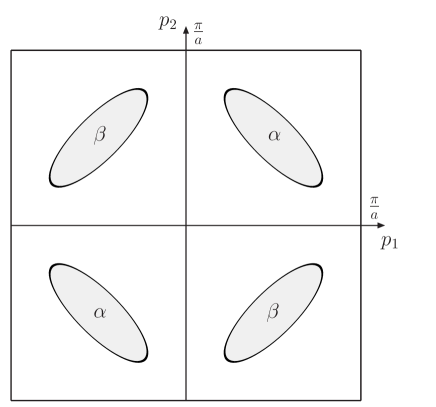
Figure 4: Elliptically shaped hole pockets centered at $(\pm\frac{\pi}{2a},\pm\frac{\pi}{2a})$. Two pockets centered at $k^{f}$ and ${k^{f}}^{\prime}$ combine to form the pockets for the flavors $f=\alpha,\beta$.

This is indeed observed both in ARPES experiments and in numerical simulations of $t$-$J$-type models (see figure 1). It should be noted that stability of the minima at the center of the hole pockets requires $|M^{\prime\prime}|>M^{\prime}$.

The leading terms with four fermion fields are given by

$${\cal L}_{4}=\sum_{s=+,-}\Big{\{} \frac{G_{1}}{2}(\psi^{\alpha\dagger}_{s}\psi^{\alpha}_{s}\psi^{\alpha\dagger}_{-s}\psi^{\alpha}_{-s}+\psi^{\beta\dagger}_{s}\psi^{\beta}_{s}\psi^{\beta\dagger}_{-s}\psi^{\beta}_{-s})$$

$$+G_{2}\psi^{\alpha\dagger}_{s}\psi^{\alpha}_{s}\psi^{\beta\dagger}_{s}\psi^{\beta}_{s}+G_{3}\psi^{\alpha\dagger}_{s}\psi^{\alpha}_{s}\psi^{\beta\dagger}_{-s}\psi^{\beta}_{-s}$$

$$+G_{4}\Big{[}\psi^{\alpha\dagger}_{s}\psi^{\alpha}_{s}\sum_{s^{\prime}=+,-}\big{(}\psi^{\beta\dagger}_{s^{\prime}}v^{s^{\prime}}_{1}\psi^{\beta}_{-s^{\prime}}-\psi^{\beta\dagger}_{s^{\prime}}v^{s^{\prime}}_{2}\psi^{\beta}_{-s^{\prime}}\big{)}$$

$$\hskip 27.0pt+\psi^{\beta\dagger}_{s}\psi^{\beta}_{s}\sum_{s^{\prime}=+,-}\big{(}\psi^{\alpha\dagger}_{s^{\prime}}v^{s^{\prime}}_{1}\psi^{\alpha}_{-s^{\prime}}+\psi^{\alpha\dagger}_{s^{\prime}}v^{s^{\prime}}_{2}\psi^{\alpha}_{-s^{\prime}}\big{)}\Big{]}\Big{\}},$$ (5.19)

with the real-valued 4-fermion contact interactions $G_{1}$, $G_{2}$, $G_{3}$, and $G_{4}$. We have limited ourselves to terms containing at most one spatial derivative. The next order contains a large number of terms with one temporal or two spatial derivatives. We have constructed these terms using the algebraic program FORM [83], but we do not list them here because they are not very illuminating. Also, due to the large number of low-energy parameters they contain, they are unlikely to be used in any practical investigation.

For completeness, we also list the contributions to the Lagrangian with six and eight fermion fields

$${\cal L}_{6}= \,H\big{(}\psi^{\alpha\dagger}_{+}\psi^{\alpha}_{+}\psi^{\alpha\dagger}_{-}\psi^{\alpha}_{-}\psi^{\beta\dagger}_{+}\psi^{\beta}_{+}+\psi^{\alpha\dagger}_{+}\psi^{\alpha}_{+}\psi^{\alpha\dagger}_{-}\psi^{\alpha}_{-}\psi^{\beta\dagger}_{-}\psi^{\beta}_{-}$$

$$\hskip 13.00005pt+\psi^{\alpha\dagger}_{+}\psi^{\alpha}_{+}\psi^{\beta\dagger}_{+}\psi^{\beta}_{+}\psi^{\beta\dagger}_{-}\psi^{\beta}_{-}+\psi^{\alpha\dagger}_{-}\psi^{\alpha}_{-}\psi^{\beta\dagger}_{+}\psi^{\beta}_{+}\psi^{\beta\dagger}_{-}\psi^{\beta}_{-}\big{)},$$

$${\cal L}_{8}= \,I\,\psi^{\alpha\dagger}_{+}\psi^{\alpha}_{+}\psi^{\alpha\dagger}_{-}\psi^{\alpha}_{-}\psi^{\beta\dagger}_{+}\psi^{\beta}_{+}\psi^{\beta\dagger}_{-}\psi^{\beta}_{-}.$$ (5.20)

Here we have limited ourselves to terms without derivatives. Terms with more fermion fields are then excluded by the Pauli principle. Again, it is straightforward to systematically construct the higher-order terms, but there is presently no need for them.

5.3 Accidental Emergent Symmetries

Interestingly, the terms in the Lagrangian constructed above have an accidental global $U(1)_{F}$ flavor symmetry that acts as

$$U(1)_{F}:\quad^{F}\psi^{f}_{\pm}(x)=\exp(\sigma_{f}i\eta)\psi^{f}_{\pm}(x).$$ (5.21)

The flavor symmetry is explicitly broken by higher-order terms in the derivative expansion and thus emerges only at low energies.

In addition, for $c\rightarrow\infty$ there is also an accidental Galilean boost symmetry $G$, which acts on the fields as

$$G: {}^{G}P(x) =P(Gx),\qquad Gx=(\vec{x}-\vec{v}\ t,t),$$

$${}^{G}\psi^{f}_{\pm}(x) =\exp\left(i\vec{p}^{f}\cdot\vec{x}-\omega^{f}t\right)\psi^{f}_{\pm}(Gx),$$

$${}^{G}\psi^{f\dagger}_{\pm}(x) =\psi^{f\dagger}_{\pm}(Gx)\exp\left(-i\vec{p}^{f}\cdot\vec{x}+\omega^{f}t\right),$$ (5.22)

with $\vec{p}^{f}=(p^{f}_{1},p^{f}_{2})$ and $\omega^{f}$ given by

$$p^{f}_{1} =\frac{M^{\prime}}{1-(M^{\prime}/M^{\prime\prime})^{2}}\left[v_{1}-\sigma_{f}\frac{M^{\prime}}{M^{\prime\prime}}v_{2}\right],\quad p^{f}_{2}=\frac{M^{\prime}}{1-(M^{\prime}/M^{\prime\prime})^{2}}\left[v_{2}-\sigma_{f}\frac{M^{\prime}}{M^{\prime\prime}}v_{1}\right],$$

$$\omega^{f} =\frac{{p^{f}_{i}}^{2}}{2M^{\prime}}+\sigma_{f}\frac{p^{f}_{1}p^{f}_{2}}{M^{\prime\prime}}=\frac{M^{\prime}}{1-(M^{\prime}/M^{\prime\prime})^{2}}\left[\frac{1}{2}(v_{1}^{2}+v_{2}^{2})-\sigma_{f}\frac{M^{\prime}}{M^{\prime\prime}}v_{1}v_{2}\right].$$ (5.23)

Note that the relation between $\vec{p}^{f}$ and the velocity of the Galilean boost $\vec{v}$ results from the hole dispersion relation of eq.(5.18) using $v_{i}=dE^{f}/dp_{i}^{f}$. Also the Galilean boost symmetry is explicitly broken at higher orders of the derivative expansion.

The fundamental physics underlying the actual cuprates is Galilean- or, in fact, even Poincaré-invariant. Poincaré symmetry is then spontaneously broken by the formation of a crystal lattice with phonons as the corresponding Nambu-Goldstone bosons. In the Hubbard or $t$-$J$ models the lattice is imposed by hand, and Galilean symmetry is thus broken explicitly instead of spontaneously. In particular, there are no phonons in these models. Remarkably, an accidental Galilean boost invariance still emerges dynamically at low energies. This has important physical consequences. In particular, without loss of generality, the hole pairs to be investigated later, can be studied in their rest frame. This is unusual for particles propagating on a lattice, because the lattice represents a preferred rest frame (a condensed matter “ether”). The accidental Galilean boost invariance may even break spontaneously, which is the case in phases with spiral configurations of the staggered magnetization.

6 Magnon-mediated Binding between Holes

Our treatment of the forces between two holes is analogous to the effective theory for light nuclei [69, 70, 71, 72] in which one-pion exchange dominates the long-range forces. In this section we calculate the one-magnon exchange potentials between holes and we solve the corresponding two-hole Schrödinger equations. The one-magnon exchange potentials as well as the solution of the Schrödinger equation for a hole pair of flavors $\alpha$ and $\beta$ were already discussed in [79]. Here we present a more detailed derivation of these results and we extend the discussion to hole pairs of the same flavor.

6.1 One-Magnon Exchange Potentials between Holes

We now calculate the one-magnon exchange potentials between holes of flavors $\alpha$ or $\beta$. For this purpose, we expand in the magnon fluctuations $m_{1}(x)$, $m_{2}(x)$ around the ordered staggered magnetization, i.e.

$$\vec{e}(x)=\Big{(}\frac{m_{1}(x)}{\sqrt{\rho_{s}}} ,\,\frac{m_{2}(x)}{\sqrt{\rho_{s}}},1\Big{)}+{\cal O}(m^{2})$$

$$\Rightarrow\quad v_{\mu}^{\pm}(x) =\frac{1}{2\sqrt{\rho_{s}}}\partial_{\mu}\big{[}m_{2}(x)\pm im_{1}(x)\big{]}+{\cal O}(m^{3}),$$

$$v_{\mu}^{3}(x) =\frac{1}{4\rho_{s}}\big{[}m_{1}(x)\partial_{\mu}m_{2}(x)-m_{2}(x)\partial_{\mu}m_{1}(x)\big{]}+{\cal O}(m^{4}).$$ (6.1)

Since vertices with $v_{\mu}^{3}(x)$ (contained in $D_{\mu}$) involve at least two magnons, one-magnon exchange results from vertices with $v_{\mu}^{\pm}(x)$ only. As a consequence, two holes can exchange a single magnon only if they have antiparallel spins ($+$ and $-$), which are both flipped in the magnon-exchange process. We denote the momenta of the incoming and outgoing holes by $\vec{p}_{\pm}$ and $\vec{p}_{\pm}\ \!\!\!\!^{\prime}\$, respectively. The momentum carried by the exchanged magnon is denoted by $\vec{q}$. We also introduce the total momentum $\vec{P}$ as well as the incoming and outgoing relative momenta $\vec{p}$ and $\vec{p}\ ^{\prime}$

$$\vec{P}=\vec{p}_{+}+\vec{p}_{-}=\vec{p}_{+}\ \!\!\!\!^{\prime}+\vec{p}_{-}\ \!\!\!\!^{\prime},$$

$$\vec{p}=\frac{1}{2}(\vec{p}_{+}-\vec{p}_{-}),\qquad\vec{p}\ ^{\prime}=\frac{1}{2}(\vec{p}_{+}\ \!\!\!\!^{\prime}-\vec{p}_{-}\ \!\!\!\!^{\prime}).$$ (6.2)

Momentum conservation then implies

$$\vec{q}=\vec{p}+\vec{p}\ ^{\prime}.$$ (6.3)

It is straightforward to evaluate the Feynman diagram describing one-magnon exchange shown in figure 5.

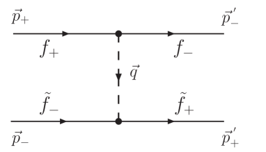
Figure 5: Feynman diagram for one-magnon exchange between two holes with antiparallel spins undergoing a spin-flip.

In momentum space the resulting potentials for the various combinations of flavors take the form

$$\langle\vec{p}_{+}\ \!\!\!\!^{\prime}\vec{p}_{-}\ \!\!\!\!^{\prime}|V^{f\tilde{f}}|\vec{p}_{+}\vec{p}_{-}\rangle=V^{f\tilde{f}}(\vec{q})\ \delta(\vec{p}_{+}+\vec{p}_{-}-\vec{p}_{+}\ \!\!\!\!^{\prime}-\vec{p}_{-}\ \!\!\!\!^{\prime}),$$ (6.4)

with

$$V^{\alpha\alpha}(\vec{q})=-\gamma\pi\frac{(q_{1}+q_{2})^{2}}{q^{2}},\qquad V^{\beta\beta}(\vec{q})=-\gamma\pi\frac{(q_{1}-q_{2})^{2}}{q^{2}},$$

$$V^{\alpha\beta}(\vec{q})=V^{\beta\alpha}(\vec{q})=-\gamma\pi\frac{q_{1}^{2}-q_{2}^{2}}{q^{2}},$$ (6.5)

where $\gamma=\Lambda^{2}/(2\pi\rho_{s})$. In coordinate space the corresponding potentials are given by

$$\langle\vec{r}_{+}\ \!\!\!\!^{\prime}\vec{r}_{-}\ \!\!\!\!^{\prime}|V^{f\tilde{f}}|\vec{r}_{+}\vec{r}_{-}\rangle=V^{f\tilde{f}}(\vec{r})\ \delta(\vec{r}_{+}-\vec{r}_{-}\ \!\!\!\!^{\prime})\ \delta(\vec{r}_{-}-\vec{r}_{+}\ \!\!\!\!^{\prime}),$$ (6.6)

with

$$V^{\alpha\alpha}(\vec{r})=\gamma\frac{\sin(2\varphi)}{r^{2}},\qquad V^{\beta\beta}(\vec{r})=-\gamma\frac{\sin(2\varphi)}{r^{2}},$$

$$V^{\alpha\beta}(\vec{r})=V^{\beta\alpha}(\vec{r})=\gamma\frac{\cos(2\varphi)}{r^{2}}.$$ (6.7)

Here $\vec{r}=\vec{r}_{+}-\vec{r}_{-}$ is the distance vector between the two holes and $\varphi$ is the angle between $\vec{r}$ and the $x$-axis. It should be noted that the one-magnon exchange potentials are instantaneous although magnons travel with the finite speed $c$. Retardation effects occur only at higher orders. The one-magnon exchange potentials also contain short-distance $\delta$-function contributions which we have not listed above. These contributions add to the 4-fermion contact interactions. Since we will model the short-distance repulsion by a hard core radius, the $\delta$-function contributions are not needed in the following.

6.2 Schrödinger Equation for two Holes of different Flavor

Let us investigate the Schrödinger equation for the relative motion of two holes with flavors $\alpha$ and $\beta$. Thanks to the accidental Galilean boost invariance, without loss of generality we can consider the hole pair in its rest frame. The total kinetic energy of the two holes is then given by

$$T=\sum_{f=\alpha,\beta}\left(\frac{p_{i}^{2}}{2M^{\prime}}+\sigma_{f}\frac{p_{1}p_{2}}{M^{\prime\prime}}\right)=\frac{p_{i}^{2}}{M^{\prime}}.$$ (6.8)

In particular, the parameter $1/M^{\prime\prime}$ that measures the deviation from a circular shape of the hole pockets drops out of the problem. The resulting Schrödinger equation then takes the form

$$\left(\begin{array}[]{cc}-\frac{1}{M^{\prime}}\Delta&V^{\alpha\beta}(\vec{r})\\[0.86108pt] V^{\alpha\beta}(\vec{r})&-\frac{1}{M^{\prime}}\Delta\end{array}\right)\left(\begin{array}[]{c}\Psi_{1}(\vec{r})\\ \Psi_{2}(\vec{r})\end{array}\right)=E\left(\begin{array}[]{c}\Psi_{1}(\vec{r})\\ \Psi_{2}(\vec{r})\end{array}\right).$$ (6.9)

The components $\Psi_{1}(\vec{r})$ and $\Psi_{2}(\vec{r})$ are probability amplitudes for the spin-flavor combinations $\alpha_{+}\beta_{-}$ and $\alpha_{-}\beta_{+}$, respectively. The potential $V^{\alpha\beta}(\vec{r})$ couples the two channels because magnon exchange is accompanied by a spin-flip. The above Schrödinger equation does not yet account for the short-distance forces arising from 4-fermion contact interactions. Their effect will be incorporated later by a boundary condition on the wave function near the origin. Making the ansatz

$$\Psi_{1}(\vec{r})\pm\Psi_{2}(\vec{r})=R(r)\chi_{\pm}(\varphi),$$ (6.10)

for the angular part of the wave function one obtains

$$-\frac{d^{2}\chi_{\pm}(\varphi)}{d\varphi^{2}}\pm M^{\prime}\gamma\cos(2\varphi)\chi_{\pm}(\varphi)=-\lambda\chi_{\pm}(\varphi).$$ (6.11)

The solutions of this Mathieu equation with the lowest eigenvalue $-\lambda$ is

$$\chi_{\pm}(\varphi)=\frac{1}{\sqrt{\pi}}\,\mbox{ce}_{0}(\varphi,\,\pm\frac{1}{2}M^{\prime}\gamma),\qquad\lambda=\frac{1}{8}(M^{\prime}\gamma)^{2}+{\cal O}(\gamma^{4}).$$ (6.12)

The periodic Mathieu function $\mbox{ce}_{0}(\varphi,\frac{1}{2}M^{\prime}\gamma)$ [84] is illustrated in figure 6.

Figure 6: Angular wave function $\mbox{ce}_{0}(\varphi,\frac{1}{2}M^{\prime}\gamma)$ (solid curve) and angle-dependence $\cos(2\varphi)$ of the potential (dotted curve) for a pair of holes with flavors $\alpha$ and $\beta$ ($M^{\prime}\gamma=2.5$).

The radial Schrödinger equation takes the form

$$-\left[\frac{d^{2}R(r)}{dr^{2}}+\frac{1}{r}\frac{dR(r)}{dr}\right]-\frac{\lambda}{r^{2}}R(r)=M^{\prime}ER(r).$$ (6.13)

As it stands, this equation is ill-defined because an attractive $\frac{1}{r^{2}}$ potential is too singular at the origin. However, we must still incorporate the contact interaction proportional to the 4-fermion couplings $G_{3}$ and $G_{4}$. A consistent description of the short-distance physics requires ultraviolet regularization and subsequent renormalization of the Schrödinger equation as discussed in [85]. In order to maintain the transparency of a complete analytic calculation, here we model the short-distance repulsion between two holes by a hard core of radius $r_{0}$, i.e. we require $R(r_{0})=0$. The radial Schrödinger equation for the bound states is solved by a Bessel function

$$R(r)=AK_{\nu}\big{(}\sqrt{M^{\prime}|E_{n}|}r\big{)},\qquad\nu=i\sqrt{\lambda}.$$ (6.14)

The energy (determined from $K_{\nu}\big{(}\sqrt{M^{\prime}|E_{n}|}r_{0}\big{)}=0$) is given by

$$E_{n}\sim-(M^{\prime}r_{0}^{2})^{-1}\exp(-2\pi n/\sqrt{\lambda})$$ (6.15)

for large $n$. As expected, the energy of the bound state depends on the values of the low-energy constants. Although the binding energy is exponentially small in $n$, for very small $r_{0}$ the ground state would have a small size and would be strongly bound. In that case, the result of the effective theory should not be trusted quantitatively, because short-distance details and not the universal magnon-dominated long-distance physics determine the structure of the bound state. Still, even in that case, an extended effective theory can be constructed which contains the tightly bound hole pairs as additional explicit low-energy degrees of freedom. For larger values of $r_{0}$, as long as the binding energy is small compared to the relevant high-energy scales such as $\rho_{s}$, the results of the effective theory in its present form are reliable, and receive only small calculable corrections from higher-order effects such as two-magnon exchange.

It should be noted that the wave functions with angular part $\chi_{+}(\varphi)$ and $\chi_{-}(\varphi)$ have the same energy. A general linear combination of the two states takes the form

$$\Psi(\vec{r})=R(r)\left(\begin{array}[]{c}a\chi_{+}(\varphi)+b\chi_{-}(\varphi)\\ a\chi_{+}(\varphi)-b\chi_{-}(\varphi)\end{array}\right).$$ (6.16)

Applying the 90 degrees rotation $O$ and using the transformation rules of eq.(5.1) one obtains

$${}^{O}\Psi(\vec{r})=R(r)\left(\begin{array}[]{c}a\chi_{+}(\varphi+\frac{\pi}{2})-b\chi_{-}(\varphi+\frac{\pi}{2})\\ -a\chi_{+}(\varphi+\frac{\pi}{2})-b\chi_{-}(\varphi+\frac{\pi}{2})\end{array}\right)=R(r)\left(\begin{array}[]{c}a\chi_{-}(\varphi)-b\chi_{+}(\varphi)\\ -a\chi_{-}(\varphi)-b\chi_{+}(\varphi)\end{array}\right).$$ (6.17)

Demanding that $\Psi(\vec{r})$ is an eigenstate of the rotation $O$, i.e. ${}^{O}\Psi(\vec{r})=o\Psi(\vec{r})$, thus implies

$$o\ a=-b,\quad o\ b=a\ \Rightarrow\ o=\pm i,$$ (6.18)

with the corresponding eigenfunctions given by

$$\Psi_{\pm}(\vec{r})=R(r)\left(\begin{array}[]{c}\chi_{+}(\varphi)\mp i\chi_{-}(\varphi)\\ \chi_{+}(\varphi)\pm i\chi_{-}(\varphi)\end{array}\right).$$ (6.19)

This leads to the probability distribution illustrated in figure 7, which resembles $d_{x^{2}-y^{2}}$ symmetry. However, unlike for a true $d$-wave, the wave function is suppressed, but not equal to zero, along the lattice diagonals. This is different for the first angular-excited state, whose wave function indeed has a node along the diagonals.

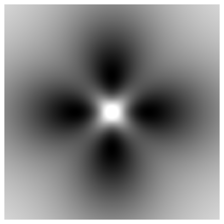
Figure 7: Probability distribution for the ground state of two holes with flavors $\alpha$ and $\beta$.

Since the problem only has a 90 degrees and not a continuous rotation symmetry, the continuum classification scheme of angular momentum eigenstates does not apply here. In fact, the 2-fold degenerate ground state belongs to the 2-dimensional irreducible representation of the group of discrete rotations and reflections. The corresponding eigenvalues of the 90 degrees rotation $O$ are $o=\pm i$.

It is also interesting to investigate the transformation properties under the reflection symmetry $R$ and the unbroken shift symmetries $D_{i}^{\prime}$. Under the reflection $R$ one obtains

$${}^{R}\Psi_{\pm}(\vec{r})=R(r)\left(\begin{array}[]{c}\chi_{+}(-\varphi)\pm i\chi_{-}(-\varphi)\\ \chi_{+}(-\varphi)\mp i\chi_{-}(-\varphi)\end{array}\right)=R(r)\left(\begin{array}[]{c}\chi_{+}(\varphi)\pm i\chi_{-}(\varphi)\\ \chi_{-}(\varphi)\mp i\chi_{+}(\varphi)\end{array}\right)=\Psi_{\mp}(\vec{r}).$$ (6.20)

Similarly, under the displacement symmetries one obtains

$${}^{D_{1}^{\prime}}\Psi_{\pm}(\vec{r})=R(r)\left(\begin{array}[]{c}\chi_{+}(\varphi)\pm i\chi_{-}(\varphi)\\ \chi_{+}(\varphi)\mp i\chi_{-}(\varphi)\end{array}\right)=\Psi_{\mp}(\vec{r}),$$ (6.23)

$${}^{D_{2}^{\prime}}\Psi_{\pm}(\vec{r})=-R(r)\left(\begin{array}[]{c}\chi_{+}(\varphi)\pm i\chi_{-}(\varphi)\\ \chi_{+}(\varphi)\mp i\chi_{-}(\varphi)\end{array}\right)=-\Psi_{\mp}(\vec{r}).$$ (6.26)

6.3 Schrödinger Equation for two Holes of the same Flavor

Let us now consider two holes of the same flavor. In particular, we focus on an $\alpha\alpha$ pair. Hole pairs of type $\beta\beta$ behave in exactly the same way. For simplicity, we first consider the (somewhat unrealistic) case of circular hole pockets. Then we discuss the realistic (but slightly more complicated) case of elliptically shaped pockets.

6.3.1 Circular Hole Pockets

Figure 8: Angular wave function $\mbox{ce}_{0}(\varphi-\frac{\pi}{4},\frac{1}{2}M^{\prime}\gamma)$ (solid curve) and angle-dependence $\sin(2\varphi)$ of the potential (dotted curve) for two holes of flavor $\alpha$ residing in a circular hole pocket ($M^{\prime}\gamma=2.5$).

Let us consider two holes of flavor $\alpha$ with opposite spins $+$ and $-$. In the rest frame the wave function depends on the relative distance vector $\vec{r}$ which points from the spin $+$ hole to the spin $-$ hole. It is important to note that magnon exchange is accompanied by a spin-flip. Hence, the vector $\vec{r}$ changes its direction in the magnon exchange process. For circular hole pockets, i.e. for $1/M^{\prime\prime}=0$, the total kinetic energy is again given by $T=p_{i}^{2}/M^{\prime}$ and the resulting Schrödinger equation takes the form

$$-\frac{1}{M^{\prime}}\Delta\Psi(\vec{r})+V^{\alpha\alpha}(\vec{r})\Psi(-\vec{r})=E\Psi(\vec{r}).$$ (6.27)

As before, we make a separation ansatz

$$\Psi(\vec{r})=R(r)\chi(\varphi).$$ (6.28)

We concentrate on the ground state which is even with respect to the reflection of $\vec{r}$ to $-\vec{r}$, i.e.

$$\chi(\varphi+\pi)=\chi(\varphi).$$ (6.29)

The angular part of the Schrödinger equation then reads

$$-\frac{d^{2}\chi(\varphi)}{d\varphi^{2}}+M^{\prime}\gamma\sin(2\varphi)\chi(\varphi)=-\lambda\chi(\varphi).$$ (6.30)

Again, this is a Mathieu equation. The ground state with eigenvalue $-\lambda$ takes the form

$$\chi(\varphi)=\frac{1}{\sqrt{\pi}}\mbox{ce}_{0}\big{(}\varphi-\frac{\pi}{4},\,\frac{1}{2}M^{\prime}\gamma\big{)},\qquad\lambda=\frac{1}{8}(M^{\prime}\gamma)^{2}+{\cal O}(\gamma^{4}).$$ (6.31)

The angular wave function for the ground state together with the angular dependence of the one-magnon exchange potential are shown in figure 8.

As before, the radial Schrödinger equation takes the form of eq.(6.13). Again, we model the short-distance repulsion between two holes by a hard core of radius $r_{0}^{\prime}$, i.e. we require $R(r_{0}^{\prime})=0$. It should be noted that $r_{0}^{\prime}$ does not necessarily take the same value as $r_{0}$ in the $\alpha\beta$ case. This is not only because there is an additional $\delta$-function contribution to the one-magnon exchange potential, but also because the 4-fermion coupling $G_{1}$ in the $\alpha\alpha$ case is in general different from the coupling $G_{3}$ in the $\alpha\beta$ case. The energy is then given by

$$E_{n}\sim-(M^{\prime}{r_{0}^{\prime}}^{2})^{-1}\exp(-2\pi n/\sqrt{\lambda})$$ (6.32)

for large $n$. Again, there are two degenerate ground states — one for an $\alpha\alpha$ and one for a $\beta\beta$ pair. They are eigenstates of flavor related to each other by a 90 degrees rotation. Since the $U(1)_{F}$ symmetry is accidental at low energies while the 90 degrees rotation symmetry is exact, it is again natural to combine the two degenerate states to eigenstates of the rotation symmetry $O$. The resulting probability distribution which resembles $d_{xy}$ symmetry is illustrated in figure 9.

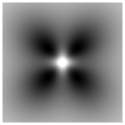
Figure 9: Probability distribution for the ground state of two holes with flavors $\alpha\alpha$ or $\beta\beta$, combined to an eigenstate of the 90 degrees rotation symmetry $O$, for the case of circular hole pockets.

As for $\alpha\beta$ pairs, the symmetry is not truly $d$-wave, but just given by the 2-dimensional irreducible representation of the group of discrete rotations and reflections. Again, the corresponding eigenvalues of the 90 degrees rotation $O$ are $o=\pm i$.

6.3.2 Elliptic Hole Pockets

Let us now move on to the realistic case of elliptically shaped hole pockets. Then the total kinetic energy of two holes of flavor $\alpha$ in their rest frame is given by

$$T=\frac{p_{i}^{2}}{M^{\prime}}+\frac{2p_{1}p_{2}}{M^{\prime\prime}}.$$ (6.33)

This suggests to rotate the coordinate system by 45 degrees such that the major axes of the ellipse are aligned with the rotated coordinate axes, i.e.

$$p_{1}^{\prime}=\frac{1}{\sqrt{2}}(p_{1}+p_{2}),\qquad p_{2}^{\prime}=\frac{1}{\sqrt{2}}(p_{1}-p_{2}).$$ (6.34)

In the rotated reference frame, the kinetic energy takes the form

$$T=\frac{{p_{1}^{\prime}}^{2}}{M_{1}}+\frac{{p_{2}^{\prime}}^{2}}{M_{2}},$$ (6.35)

with

$$\frac{1}{M_{1}}=\frac{1}{M^{\prime}}+\frac{1}{M^{\prime\prime}},\qquad\frac{1}{M_{2}}=\frac{1}{M^{\prime}}-\frac{1}{M^{\prime\prime}}.$$ (6.36)

It is convenient to rescale the rotated axes such that the hole pocket again assumes a circular shape. This is achieved by defining

$$\widetilde{p}_{1}=\sqrt{\frac{M^{\prime}}{M_{1}}}p_{1}^{\prime},\qquad\widetilde{p}_{2}=\sqrt{\frac{M^{\prime}}{M_{2}}}p_{2}^{\prime},$$ (6.37)

which indeed implies

$$T=\frac{\widetilde{p}_{1}^{2}}{M^{\prime}}+\frac{\widetilde{p}_{2}^{2}}{M^{\prime}}=\frac{\widetilde{p}_{i}^{2}}{M^{\prime}},$$ (6.38)

just as for the circular hole pocket. Of course, the rotation and rescaling must also be applied to the coordinates, i.e.

$$\widetilde{x}_{1}=\sqrt{\frac{M_{1}}{2M^{\prime}}}(x_{1}+x_{2})=\widetilde{r}\cos\widetilde{\varphi},\qquad\widetilde{x}_{2}=\sqrt{\frac{M_{2}}{2M^{\prime}}}(x_{1}-x_{2})=\widetilde{r}\sin\widetilde{\varphi}.$$ (6.39)

The rotated and rescaled one-magnon exchange potential then takes the form

$$V^{\alpha\alpha}(\widetilde{\vec{r}}) = \gamma\frac{\sin(2\varphi)}{r^{2}}=\gamma\frac{2x_{1}x_{2}}{(x_{1}^{2}+x_{2}^{2})^{2}}=\gamma\frac{\widetilde{x}_{1}^{2}\,M^{\prime}/M_{1}-\widetilde{x}_{2}^{2}\,M^{\prime}/M_{2}}{(\widetilde{x}_{1}^{2}\,M^{\prime}/M_{1}+\widetilde{x}_{2}^{2}\,M^{\prime}/M_{2})^{2}}$$ (6.40)

$$= \gamma\frac{\cos(2\widetilde{\varphi})+M^{\prime}/M^{\prime\prime}}{{\widetilde{r}}^{2}(1+\cos(2\widetilde{\varphi})\,M^{\prime}/M^{\prime\prime})^{2}},$$

and the corresponding Schrödinger equation reads

$$-\frac{1}{M^{\prime}}\Delta\Psi(\widetilde{\vec{r}})+V^{\alpha\alpha}(\widetilde{\vec{r}})\Psi(-\widetilde{\vec{r}})=E\Psi(\widetilde{\vec{r}}).$$ (6.41)

Once again, we make the separation ansatz

$$\Psi(\widetilde{\vec{r}})=R(\widetilde{r})\chi(\widetilde{\varphi}),$$ (6.42)

such that the angular part of the Schrödinger equation now takes the form

$$-\frac{d^{2}\chi(\widetilde{\varphi})}{d\widetilde{\varphi}^{2}}+M^{\prime}\gamma\frac{\cos(2\widetilde{\varphi})+M^{\prime}/M^{\prime\prime}}{(1+\cos(2\widetilde{\varphi})\,M^{\prime}/M^{\prime\prime})^{2}}\chi(\widetilde{\varphi})=-\lambda\chi(\widetilde{\varphi}).$$ (6.43)

This is a differential equation in the class of Hill equations [86] which we have solved numerically. Figure 10 shows the angular wave function for the ground state together with the angular dependence of the rotated and rescaled one-magnon exchange potential.

Figure 10: Angular wave function (solid curve) and angle-dependence of the rotated and rescaled one-magnon exchange potential (dotted curve) for two holes of flavor $\alpha$ in an elliptic hole pocket (for $M^{\prime}/M^{\prime\prime}=0.5$ and $M^{\prime}\gamma=2.5$).

The radial Schrödinger equation takes exactly the same form as for circular hole pockets and will therefore not be discussed again. There are two degenerate states corresponding to $\alpha\alpha$ and $\beta\beta$ pairs, which are related to each other by a 90 degrees rotation. Combining the two degenerate states to an eigenstate of the rotation $O$, one obtains the probability distribution of figure 11 which again resembles $d_{xy}$ symmetry.

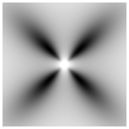
Figure 11: Probability distribution for the ground state of two holes with flavors $\alpha\alpha$ or $\beta\beta$ in elliptic hole pockets, linearly combined to an eigenstate of the 90 degrees rotation $O$.

Qualitatively similar results for hole pairs from the same hole pocket were obtained in [29] directly from the $t$-$J$ model, however, using some uncontrolled approximations. The effective field theory treatment has the advantage of being systematic, i.e. it can be improved order by order in the derivative expansion. Besides this, the effective field theory approach is particularly transparent and conceptually simple.

6.4 Low-Energy Dynamics of Hole Pairs

As we have seen, magnons mediate attractive forces between holes of opposite spin which leads to bound states with $d$-wave characteristics. Once pairs of holes have formed, it is natural to ask how they behave at low temperatures. It should be stressed that, until now, we have considered isolated hole pairs in an otherwise undoped antiferromagnet. What should one expect when the system is doped with a non-zero density of holes? First of all, even for infinitesimal doping, the antiferromagnet may become unstable against the formation of inhomogeneities, such as spirals in the staggered magnetization [6]. This phenomenon can be studied within the effective theory and is presently under investigation [80]. It turns out that, for sufficiently large spin stiffness $\rho_{s}$, the homogeneous antiferromagnet is stable, while for intermediate values of $\rho_{s}$ it becomes unstable against the formation of a spiral phase. For even smaller values of $\rho_{s}$, the spiral itself becomes unstable against the formation of further, yet unidentified, inhomogeneities. In the following, we will assume a sufficiently large value of $\rho_{s}$ such that the homogeneous antiferromagnet is stable.

If the short-range repulsion is particularly strong in the $\alpha\alpha$ and $\beta\beta$ channels, hole pairs of type $\alpha\beta$ with $d_{x^{2}-y^{2}}$-like symmetry are most strongly bound. On the other hand, if the short-range repulsion is stronger in the $\alpha\beta$ channel, $\alpha\alpha$ or $\beta\beta$ pairs form and the symmetry resembles $d_{xy}$. At very low densities and temperatures, the hole pairs form a dilute system of bosons. In this case, the wave functions of different pairs do not overlap substantially, and it is natural to assume that they may undergo Bose-Einstein condensation at sufficiently low temperatures. At larger densities, the wave functions of different pairs begin to overlap. In that case, a momentum space description of holes is more appropriate. Magnon exchange between holes near the Fermi surface is then likely to produce an instability against Cooper pair formation in the $d$-wave channel. This is expected to lead to BCS-type superconductivity, mediated by magnons instead of phonons. Using the effective theory, the critical temperature for magnon-mediated BCS-type superconductivity will be calculated elsewhere, but is not expected to be very high. In particular, superconductivity coexisting with antiferromagnetism at low doping is not observed in the cuprates. This may well be due to impurities on which holes get localized, thus preventing superconductivity. Magnon-mediated superconductivity in lightly doped antiferromagnets can still be studied systematically using the effective field theory which does not contain impurities.

7 Conclusions

Based on a careful symmetry analysis of the Hubbard and $t$-$J$ models, we have constructed a systematic low-energy effective field theory for magnons and holes in lightly doped antiferromagnets. The effective theory provides a powerful framework in which nontrivial aspects of the strongly coupled dynamics of the cuprates, such as the magnon-mediated forces between holes, can be addressed using systematic methods of weak coupling perturbation theory. The effective theory relies on a number of basic assumptions. Besides fundamental principles of field theory, such as locality, unitarity, and symmetry, it is based on the assumption that the $SU(2)_{s}$ spin symmetry is spontaneously broken down to $U(1)_{s}$. This assumption is very accurately verified both in experiments with the cuprates and by numerical calculations in the Hubbard and $t$-$J$ model at half-filling. A second basic assumption is that fermionic quasi-particles — the holes of the effective theory — indeed exist as stable excitations located in specific pockets in the Brillouin zone. The location of these pockets in momentum space has been obtained from ARPES measurements as well as from numerical computations in Hubbard and $t$-$J$ models. It should be stressed that the applicability of the effective theory depends crucially on the question if the relevant low-energy degrees of freedom have indeed been identified correctly. Since it is impossible to rigorously derive the effective theory from an underlying microscopic system, we can not yet be completely sure that our effective theory indeed describes their low-energy physics correctly. In order to verify the correctness and accuracy of the effective theory, besides the theoretical considerations presented here, it will be important to confront it with experimental or numerical data. For undoped antiferromagnets, such confrontation led to a spectacular quantitative success of the pure magnon effective theory [87, 88]. It is expected that the full effective theory including holes will be equally successful. An important next step will be the comparison with precise Monte Carlo data, e.g.  for the $t$-$J$ model. This will allow us to fix the values of the low-energy parameters of the effective theory in terms of the microscopic parameters $t$ and $J$.

The effective theory can be used to calculate a wide variety of physical processes. The most basic processes include, for example, magnon-magnon and magnon-hole scattering. In order to correct the leading-order tree-level diagrams by a systematic loop expansion, in analogy to chiral perturbation theory, a power-counting scheme must be constructed. This is straightforward in the pure-magnon effective theory and should be generalized to the full effective theory including charge carriers along the lines of [54]. We have performed a systematic effective field theory analysis of the magnon-mediated forces between holes in an antiferromagnet. One-magnon exchange mediates forces exclusively between holes of opposite spin. The leading terms in the fermionic part of the effective action are Galilean boost invariant and the two-hole system can thus be studied in its rest frame. Remarkably, some of the resulting two-particle Schrödinger equations can be solved completely analytically. Hole-doped cuprates have hole pockets centered at lattice momenta $k^{\alpha}=(\frac{\pi}{2a},\frac{\pi}{2a})$ and $k^{\beta}=(\frac{\pi}{2a},-\frac{\pi}{2a})$. As a consequence, the holes carry a “flavor”-index $f=\alpha,\beta$ which specifies the pocket to which a hole belongs. At leading order, flavor is a conserved quantum number, and one can thus distinguish hole pairs of the types $\alpha\alpha$ or $\beta\beta$ from those of type $\alpha\beta$. Magnon exchange occurs with the same strength for both types, and leads to bound hole pairs with $d$-wave symmetry. For pairs of type $\alpha\alpha$ or $\beta\beta$ the symmetry resembles $d_{xy}$, while for those of type $\alpha\beta$ it is $d_{x^{2}-y^{2}}$-like. Depending on the strength of the respective short-distance repulsion either the pairs of type $\alpha\alpha$ and $\beta\beta$ or those of type $\alpha\beta$ are more strongly bound. At low densities and temperatures, the hole pairs may undergo Bose-Einstein condensation. Once the wave functions of different pairs overlap substantially, one may expect BCS-type magnon-mediated $d$-wave superconductivity coexisting with antiferromagnetism. Although coexistence of antiferromagnetism and superconductivity is not observed in the cuprates — possibly due to the localization of holes on impurities — the exchange of spin fluctuations is a promising potential mechanism for high-temperature superconductivity. In lightly doped systems without impurities, magnon-mediated superconductivity can be studied systematically using the effective theory. Other applications of the effective theory, which are currently under investigation, aim at a quantitative understanding of the destruction of antiferromagnetism upon doping and of the generation of spiral phases [80].

It is also natural to ask if the effective theory can possibly be applied to the high-temperature superconductors themselves. Since in the real materials, which contain impurities, high-temperature superconductivity arises only after antiferromagnetism has been destroyed, and since the effective theory relies on the spontaneous breakdown of the $SU(2)_{s}$ symmetry, this seems doubtful. However, while the systematic treatment of the effective theory will break down in the superconducting phase, the effective theory itself does not, as long as spin fluctuations (now with a finite correlation length) and holes in momentum space pockets $(\frac{\pi}{2a},\pm\frac{\pi}{2a})$ remain the relevant degrees of freedom. After all, the effective theory of magnons and holes can also be considered beyond perturbation theory, for example, by regularizing it on a lattice and simulating it numerically. A similar procedure has been discussed for the effective theory of pions and nucleons [89]. Unfortunately, one would expect that the sign problem will once more raise its ugly head, and may thus prevent efficient numerical simulations not only in the microscopic models but also in the effective theory. It thus remains to be seen if nonperturbative investigations of the effective theory can shed light on the phenomenon of high-temperature superconductivity itself. We prefer to first concentrate on lightly doped systems without impurities for which the low-energy effective field theory makes quantitative predictions. Once these idealized systems are better understood, further steps towards understanding the more complicated actual materials can be taken on a more solid theoretical basis.

References

- [1] J. C. Bednorz and K. A. Müller, Z. Phys. B64 (1986) 189.
- [2] W. F. Brinkman and T. M. Rice, Phys. Rev. B2 (1970) 1324.
- [3] J. E. Hirsch, Phys. Rev. Lett. 54 (1985) 1317.
- [4] P. W. Anderson, Science 235 (1987) 1196.
- [5] C. Gros, R. Joynt, and T. M. Rice, Phys. Rev. B36 (1987) 381.
- [6] B. I. Shraiman and E. D. Siggia, Phys. Rev. Lett. 60 (1988) 740; Phys. Rev. Lett. 61 (1988) 467; Phys. Rev. Lett. 62 (1989) 1564; Phys. Rev. B46 (1992) 8305.
- [7] S. A. Trugman, Phys. Rev. B37 (1988) 1597.
- [8] J. R. Schrieffer, X. G. Wen, and S. C. Zhang, Phys. Rev. Lett. 60 (1988) 944; Phys. Rev. B39 (1989) 11663.
- [9] C. L. Kane, P. A. Lee, and N. Read, Phys. Rev. B39 (1989) 6880.
- [10] S. Sachdev, Phys. Rev. B39 (1989) 12232.
- [11] X. G. Wen, Phys. Rev. B39 (1989) 7223.
- [12] A. Krasnitz, E. G. Klepfish, and A. Kovner, Phys. Rev. B39 (1989) 9147.
- [13] R. Shankar, Phys. Rev. Lett. 63 (1989) 203; Nucl. Phys. B330 (1990) 433.
- [14] P. W. Anderson, Phys. Rev. Lett. 64 (1990) 1839.
- [15] A. Singh and Z. Tesanovic, Phys. Rev. B41 (1990) 614.
- [16] S. A. Trugman, Phys. Rev. B41 (1990) 892.
- [17] V. Elser, D. A. Huse, B. I. Shraiman, and E. D. Siggia, Phys. Rev. B41 (1990) 6715.
- [18] E. Dagotto, R. Joynt, A. Moreo, S. Bacci, and E. Gagliano, Phys. Rev. B41 (1990) 9049.
- [19] G. Vignale and M. R. Hedayati, Phys. Rev. B42 (1990) 786.
- [20] P. Kopietz, Phys. Rev. B42 (1990) 1029.
- [21] H. J. Schulz, Phys. Rev. Lett. 65 (1990) 2462.
- [22] Z. Y. Weng, C. S. Ting, and T. K. Lee, Phys. Rev. B43 (1991) 3790.
- [23] J. A. Verges, E. Louis, P. S. Lomdahl, F. Guinea, and A. R. Bishop, Phys. Rev. B43 (1991) 6099.
- [24] F. Marsiglio, A. E. Ruckenstein, S. Schmitt-Rink, and C. M. Varma, Phys. Rev. B43 (1991) 10882.
- [25] P. Monthoux, A. V. Balatsky, and D. Pines, Phys. Rev. Lett. 67 (1991) 3448.
- [26] Z. Liu and E. Manousakis, Phys. Rev. B45 (1992) 2425.
- [27] C. Kübert and A. Muramatsu, Phys. Rev. B47 (1993) 787; cond-mat/9505105.
- [28] T. Dahm, J. Erdmenger, K. Scharnberg, and C. T. Rieck, Phys. Rev. B48 (1993) 3896.
- [29] M. Y. Kuchiev and O. P. Sushkov, Physica C218 (1993) 197.
- [30] V. V. Flambaum, M. Y. Kuchiev, and O. P. Sushkov, Physica C227 (1994) 467.
- [31] O. P. Sushkov, Phys. Rev. B49 (1994) 1250.
- [32] E. Dagotto, Rev. Mod. Phys. 66 (1994) 763.
- [33] V. I. Belinicher, A. L. Chernychev, A. V. Dotsenko, and O. P. Sushkov, Phys. Rev. B51 (1994) 6076.
- [34] J. Altmann, W. Brenig, A. P. Kampf, and E. Müller-Hartmann, Phys. Rev. B52 (1995) 7395.
- [35] B. Kyung and S. I. Mukhin, Phys. Rev. B55 (1997) 3886.
- [36] A. V. Chubukov and D. K. Morr, Phys. Rev. B57 (1998) 5298.
- [37] N. Karchev, Phys. Rev. B57 (1998) 10913.
- [38] W. Apel, H.-U. Everts, and U. Körner, Eur. Phys. J. B5 (1998) 317.
- [39] M. Brunner, F. F. Assaad, and A. Muramatsu, Phys. Rev. B62 (2000) 15480.
- [40] A. S. Mishchenko, N. V. Prokof’ev, and B. V. Svistunov, cond-mat/0103234.
- [41] S. Sachdev, Rev. Mod. Phys. 75 (2003) 913; Annals Phys. 303 (2003) 226.
- [42] O. P. Sushkov and V. N. Kotov, Phys. Rev. B70 (2004) 024503.
- [43] V. N. Kotov and O. P. Sushkov, Phys. Rev. B70 (2004) 195105.
- [44] S. Chakravarty, B. I. Halperin, and D. R. Nelson, Phys. Rev. B39 (1989) 2344.
- [45] S. Weinberg, Physica 96 A (1979) 327.
- [46] J. Gasser and H. Leutwyler, Nucl. Phys. B250 (1985) 465.
- [47] F. Kämpfer, M. Moser, and U.-J. Wiese, Nucl. Phys. B729 (2005) 317.
- [48] S. Coleman, J. Wess, and B. Zumino, Phys. Rev. 177 (1969) 2239.
- [49] C. G. Callan, S. Coleman, J. Wess, and B. Zumino, Phys. Rev. 177 (1969) 2247.
- [50] H. Georgi, Weak Interactions and Modern Particle Theory, Benjamin-Cummings Publishing Company, 1984.
- [51] J. Gasser, M. E. Sainio, and A. Svarc, Nucl. Phys. B307 (1988) 779.
- [52] E. Jenkins and A. Manohar, Phys. Lett. B255 (1991) 558.
- [53] V. Bernard, N. Kaiser, J. Kambor, and U.-G. Meissner, Nucl. Phys. B388 (1992) 315.
- [54] T. Becher and H. Leutwyler, Eur. Phys. J. C9 (1999) 643.
- [55] H. Neuberger and T. Ziman, Phys. Rev. B39 (1989) 2608.
- [56] D. S. Fisher, Phys. Rev. B39 (1989) 11783.
- [57] P. Hasenfratz and H. Leutwyler, Nucl. Phys. B343 (1990) 241.
- [58] P. Hasenfratz and F. Niedermayer, Phys. Lett. B268 (1991) 231.
- [59] P. Hasenfratz and F. Niedermayer, Z. Phys. B92 (1993) 91.
- [60] A. Chubukov, T. Senthil, and S. Sachdev, Phys. Rev. Lett. 72 (1994) 2089; Nucl. Phys. B426 (1994) 601.
- [61] H. Leutwyler, Phys. Rev. D49 (1994) 3033.
- [62] C. P. Hofmann, Phys. Rev. B60 (1999) 388; Phys. Rev. B60 (1999) 406; cond-mat/0106492; cond-mat/0202153.
- [63] J. M. Roman and J. Soto, Int. J. Mod. Phys. B13 (1999) 755; Ann. Phys. 273 (1999) 37; Phys. Rev. B59 (1999) 11418; Phys. Rev. B62 (2000) 3300.
- [64] O. Bär, M. Imboden, and U.-J. Wiese, Nucl. Phys. B686 (2004) 347.
- [65] B. O. Wells, Z.-X. Shen, D. M. King, M. H. Kastner, M. Greven, and R. J. Birgeneau, Phys. Rev. Lett. 74 (1995) 964.
- [66] S. La Rosa, I. Vobornik, F. Zwick, H. Berger, M. Grioni, G. Margaritondo, R. J. Kelley, M. Onellion, and A. Chubukov, Phys. Rev. B56 (1997) R525.
- [67] C. Kim, P. J. White, Z.-X. Shen, T. Tohyama, Y. Shibata, S. Maekawa, B. O. Wells, Y. J. Kim, R. J. Birgeneau, and M. A. Kastner, Phys. Rev. Lett. 80 (1998) 4245.
- [68] F. Ronning, C. Kim, D. L. Feng, D. S. Marshall, A. G. Loeser, L. L. Miller, J. N. Eckstein, I. Borovic, and Z. X. Shen, Science 282 (1998) 2067.
- [69] S. Weinberg, Phys. Lett. B251 (1990) 288; Nucl. Phys. B363 (1991) 3; Phys. Lett. B295 (1992) 114.
- [70] D. B. Kaplan, M. J. Savage, and M. B. Wise, Phys. Lett. B424 (1998) 390; Nucl. Phys. B534 (1998) 329.
- [71] E. Epelbaum, W. Glöckle, and U.-G. Meissner, Nucl. Phys. A637 (1998) 107; Nucl. Phys. A684 (2001) 371; Nucl. Phys. A714 (2003) 535.
- [72] P. F. Bedaque, H.-W. Hammer, and U. van Kolck, Phys. Rev. C58 (1998) 641; Phys. Rev. Lett. 82 (1999) 463; Nucl. Phys. A676 (2000) 357.
- [73] U. van Kolck, Prog. Part. Nucl. Phys. 43 (1999) 337.
- [74] T.-S. Park, K. Kubodera, D.-P. Min, and M. Rho, Nucl. Phys. A646 (1999) 83.
- [75] E. Epelbaum, H. Kamada, A. Nogga, H. Witali, W. Glöckle, and U.-G. Meissner, Phys. Rev. Lett. 86 (2001) 4787.
- [76] S. Beane, P. F. Bedaque, M. J. Savage, and U. van Kolck, Nucl. Phys. A700 (2002) 377.
- [77] P. F. Bedaque and U. van Kolck, Ann. Rev. Nucl. Part. Sci. 52 (2002) 339.
- [78] A. Nogga, R. G. E. Timmermans, and U. van Kolck, Phys. Rev. C72 (2005) 054006.
- [79] C. Brügger, F. Kämpfer, M. Pepe, and U.-J. Wiese, cond-mat/0511367.
- [80] C. Brügger, C. Hofmann, F. Kämpfer, M. Pepe, and U.-J. Wiese, in preparation.
- [81] S. Zhang, Phys. Rev. Lett. 65 (1990) 120.
- [82] C. N. Yang and S. Zhang, Mod. Phys. Lett. B4 (1990) 759.
- [83] J. A. M. Vermaseren, “New Features of FORM”, math-ph/0010025.
- [84] M. Abramowitz and I. A. Stegun, Handbook of Mathematical Functions, Dover Publications, Inc., New York.
- [85] G. P. Lepage, nucl-th/9706029.
- [86] W. Magnus, “Hills’s equation”, Dover Publications, 1966.
- [87] U.-J. Wiese and H.-P. Ying, Z. Phys. B93 (1994) 147.
- [88] B. B. Beard and U.-J. Wiese, Phys. Rev. Lett. 77 (1996) 5130.
- [89] S. Chandrasekharan, M. Pepe, F. Steffen, and U.-J. Wiese, JHEP 0312 (2003) 035.