Dynamics of molecular nanomagnets in time-dependent external magnetic fields:
Beyond the Landau-Zener-Stückelberg model

Abstract

The time evolution of the magnetization of a magnetic molecular crystal is obtained in an external time-dependent magnetic field, with sweep rates in the kT/s range. We present the ’exact numerical’ solution of the time dependent Schrödinger equation, and show that the steps in the hysteresis curve can be described as a sequence of two-level transitions between adiabatic states. The multilevel nature of the problem causes the transition probabilities to deviate significantly from the predictions of the Landau-Zener-Stückelberg model. These calculations allow the introduction of an efficient approximation method that accurately reproduces the exact results. When including phase relaxation by means of an appropriate master equation, we observe an interplay between coherent dynamics and decoherence. This decreases the size of the magnetization steps at the transitions, but does not modify qualitatively the physical picture obtained without relaxation.

I Introduction

There has been an increased interest in the study of crystals consisting of high-spin molecules such as Mn₁₂-Ac and Fe₈O. These organic molecules, also known as molecular nanomagnets,Gatteschi et al. (2006) contain transition metal atoms with strongly exchange-coupled spins, which causes the individual molecules to behave as a single, large spin. Experiments on the magnetization dynamics of these molecular crystals have shown the presence of a series of steps in the hysteresis curve at sufficiently low temperatures.Friedman et al. (1996); Mertes et al. (2001); Wernsdorfer et al. (2006) This behavior is a consequence of quantum mechanical tunneling of spin states through the anisotropy energy barrier and occurs when the external field brings two levels at different sides of the barrier into resonance. This macroscopic quantum effect has been the subject of intensive experimental and theoretical investigation which revealed additional remarkable properties of the magnetic molecules. In particular, it has been demonstrated that the magnetic tunneling could be accompanied by the emission of electromagnetic radiation, and bursts of microwave pulses have been detected in recent experiments.Tejada et al. (2004); Vanacken et al. (2004); Hernandez-Minguez et al. (2005) It has been proposed that the physical mechanism responsible for this radiation is a collective quantum effect known as superradiance.Dicke (1954); Benedict et al. (1996); Chudnovsky and Garanin (2002); Henner and Kaganov (2003); Joseph et al. (2004) This interpretation has been questioned and it was argued that when one includes the time scale of relaxation, a maser-like effect is more likely responsible for the observations.Benedict et al. (2005) Furthermore, the change in magnetization can be described in terms of avalanches, which were recently shown to propagate through the crystal in an analogous way to that of a flame front in a flammable chemical substance (deflagration).Suzuki et al. (2005); Hernandez-Mínguez et al. (2005) It has also been suggestedLeuenberger and Loss (2001) that these molecules can be used for implementing a quantum computational algorithm.

In this work we study the dynamics of the multilevel system corresponding to the $21$ spin states of the Mn₁₂-Ac molecule ($S=10$) in a time-dependent magnetic field. An ’exact numerical’ solution of the relevant time-dependent Schrödinger equation is obtained in the whole time interval of interest. The results show that, although the usual qualitative picture of consecutive two-level transitions holds, the transition probabilities deviate significantly from the predictions of the Landau-Zener-StückelbergLandau (1932); Zener (1932); Stückelberg (1932) (LZS) model. This deviation is closely related to the multilevel nature of the problem: examples are given where the single relevant parameter of the LZS model (which is essentially the level splitting in appropriate units) is the same, but the transition probabilities are different due to the different time dependence of the adiabatic energy levels. An efficient approximation method based on non-LZS two-level transitions is introduced, which is able to describe the dynamics with high accuracy. Furthermore, relaxation effects are also included. By considering realistic dephasing rates, it is shown that for field sweep rates in the kT/s range, neither unitary time evolution nor relaxation dominates the dynamics. The interplay between these two processes results in a decrease of the transition probability at a given avoided level crossing.

The paper is organized as follows: In Sec. II the relevant Hamiltonian is discussed, along with its level structure, and the dynamical equations in the adiabatic basis are introduced. Results related to the solution of the time dependent Schrödinger equation are presented in Sec. III, and the consequences of relaxation effects are discussed in Sec. IV. Finally in Sec. V the results are summarized and conclusions are presented.

II Magnetic level structure and dynamical equations

ExperimentalFriedman et al. (1996); Mertes et al. (2001); Mirebeau et al. (1999); Barra et al. (1997); Hill et al. (1998, 2003) studies on crystals of Mn₁₂Ac and Fe₈O suggest that the spin Hamiltonian for these systems can be written as

$$H_{S}(t)=H_{0}(t)+H_{1}(t),$$ (1)

where $H_{0}$ is diagonal in the eigenbasis $\{|m\rangle\}$ of the $z$ component of the spin operator, $S_{z}$:

$$H_{0}(t)=-DS_{z}^{2}-FS_{z}^{4}-g\mu_{B}B(t)S_{z}.$$ (2)

Here the last term in the right-hand side describes the coupling to an external magnetic field applied along the $z$ direction, which is parallel with the easy axis of the crystal. This external field is time-dependent, with sweep rates on the kT/s scale.Vanacken et al. (2004) $H_{1}$ in the Hamiltonian contains termsMertes et al. (2001); Barra et al. (1997) that do not commute with $S_{z}$:

$$H_{1}=C(S_{+}^{4}+S_{-}^{4})+E(S_{+}^{2}+S_{-}^{2})/2+K(S_{+}+S_{-})/2.$$ (3)

In the present paper we will concentrate on Mn₁₂-Ac, which can be considered as a representative example of molecular nanomagnets. In this case the values of the parameters in $H_{0}$ are $D/k_{B}=0.56K,$ and $F/k_{B}=1.1\cdot 10^{-3}K$. The coefficients in $H_{1}$, which are essential for the determination of the transition probabilities, can be obtained by fitting the theoretical results to experimental magnetization curves.Benedict et al. (2005) In this paper we use $K=0.025g\mu_{B}B$, $E/k_{B}=-4.48$ $10^{-3}$ $K$, $C/k_{B}=1.7$ $10^{-5}$ $K$ unless otherwise stated.

Considering the total Hamiltonian (1) as the generator of the time evolution, the corresponding time-dependent Schrödinger equation governs the dynamics. We can also use a density operator $\varrho$ to describe the system and write

$$\frac{\partial\varrho}{\partial t}=-{i}\left[H_{S},\varrho\right],$$ (4)

where $\hbar=1$. Relaxation effects can then be included through additional terms on the right hand side of this equation, see Sec. IV for more details.

A direct calculation of the time-dependent solutions of Eq. (4) when expanded in the $\{|m\rangle\}$ eigenbasis of the spin operator $S_{z}$ turns out to be a rather difficult problem: even for large field sweep rates (i.e, kT/s), the saturation of the magnetization is reached in a few milliseconds. During this time, roughly $10^{9}$ Bohr oscillations take place due to $H_{0}$, raising demanding requirements on the accuracy of the numerical process. An alternative and more efficient way of dealing with this equation is based on the expansion of the time-dependent states in an adiabatic basis, i.e., the basis of the instantaneous eigenstates of $H_{S}(t)$:

$$H_{S}(t)\left|E_{n}(t)\right\rangle=E_{n}(t)\left|E_{n}(t)\right\rangle.$$ (5)

It is convenient to label these states so that they correspond to the eigenenergies in increasing order: $E_{0}(t)<E_{1}(t)<\ldots<E_{20}(t)$ at all times. The energy curves $E_{n}(t)$ are thus continuous. It must be stressed that the time dependence of these states is parametrical. In fact they are in a one-to-one correspondence with the external field, and thus the value of the time-dependent $B$ completely determines the states $\left|E_{n}\right\rangle$. Next, the density operator is expanded in the time-dependent basis determined by Eq. (5):

$$\varrho(t)=\sum_{nm}e^{i\int_{t_{0}}^{t}(E_{m}-E_{n})dt^{\prime}}\rho_{nm}(t)\left|E_{n}(t)\right\rangle\left\langle E_{m}(t)\right|.$$ (6)

Using Eq. (4) to calculate the dynamics, and Eq. (5) to obtain the time dependence of the adiabatic states, one finds that the time evolution of the matrix $\rho$ takes the form of a von Neumann equation

$$\frac{\partial\rho}{\partial t}=-i\left[\widetilde{H},\rho\right],$$ (7)

where $\widetilde{H}$ is given by

$$\widetilde{H}_{nm}(t)=i\left\langle E_{n}\right|\frac{\partial H_{S}}{\partial t}\left|E_{m}\right\rangle\frac{e^{i\int_{t_{0}}^{t}(E_{n}-E_{m})dt^{\prime}}}{E_{n}(t)-E_{m}(t)},$$ (8)

if $n\neq m$, and $\widetilde{H}_{nn}=0.$ This expression explicitly shows that an appreciable change in the populations $\rho_{nn}$ and $\rho_{mm}$ is expected around the avoided crossing of the levels $E_{n}$ and $E_{m}$, i.e., when the denominator in Eq. (8) has a local minimum. A qualitatively similar conclusion follows from a degenerate perturbation calculationvan Vleck (1929); des Cloizeaux (1960); Klein (1974); Garanin (1991); Leuenberger and Loss (2000); Yoo and Park (2005); Benedict et al. (2005) around the avoided level crossings; but note that Eq. (8) is an exact result.

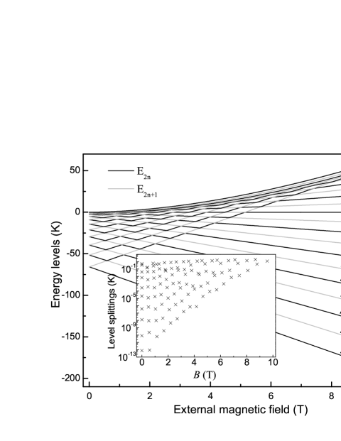
Figure 1: The level scheme of the Hamiltonian (1) as a function of the external magnetic field $B$. The energy levels corresponding to the exact eigenstates $\left|E_{n}\right\rangle$ have ”zigzag” form, while the approximate eigenenergies corresponding to the eigenstates of $S_{z}$ are almost straight lines (with periodically changing black and grey sections) for low energies. (A few examples are labeled in the figure.) The inset shows the minimal distance between levels as a function of $B,$ the horizontal position of the crosses coincide the avoided level crossings shown in the main part of the figure.

The level scheme and the minimal energy difference between levels at the avoided crossings are shown in Fig. 1. As a guiding line, far from the crossings we can associate a label $m$ to each energy eigenvalue $E_{n}$ in such a way that the overlap $|\langle m\left|E_{n}\right\rangle|$ is maximal over all possible values of $m$ between -10 and 10. This assignment is based on the fact that $H_{1}$ is a relatively weak perturbation to $H_{0},$ thus – at least for low energies and far from the crossings – the eigenstates of the full spin Hamiltonian are close to that of $H_{0}.$ As a consequence of the labelling convention introduced after Eq. (5), a given adiabatic eigenstate $\left|E_{n}\right\rangle$ before and after the avoided crossing of the levels $E_{n}$ and $E_{n\pm 1}$ corresponds to two different states $|m\rangle\neq|m^{\prime}\rangle$, see Fig. 1. In other words, if the population corresponding to a certain adiabatic state does not change while passing a crossing, the expectation value of $S_{z}$ and thus the magnetization does change.

The fact that the level splittings at the avoided crossings can differ by 12 orders of magnitude, raises an additional difficulty when using Eq. (7) to calculate the dynamics, because the derivatives also change in a similarly wide range. Therefore it turned out that a combination of Eqs. (4) and (7) leads to the most efficient method: when some populated levels are too close to each other, Eq. (7) is no longer able to provide the required accuracy, therefore we change the basis and use Eq. (4) for a short time interval after which it will be safe again to work with Eq. (7). Thus the control parameter defining the stepsize needed to have the required accuracy for such a long calculation is essentially the minimal distance between the populated levels.

The dynamical equation (7) indicates that the usual approach of treating the problem as a sequence of two-level transitions (each taking place at the corresponding level crossing) may provide an accurate approximation to the time evolution. In this framework the dynamics of the states corresponding to the anticrossing levels is governed by a $2\times 2$ Hamiltonian resulting from the reductionvan Vleck (1929); des Cloizeaux (1960); Klein (1974); Garanin (1991); Leuenberger and Loss (2000); Yoo and Park (2005); Benedict et al. (2005) of the complete $H_{S}$ to the relevant level pairs. Additionally, in this approach it is usually assumed that the time dependence of the diagonal elements of the reduced Hamiltonian is linear, while the offdiagonal ones are constants:

$$H_{red}(t)=\hbar\left(\begin{array}[]{cc}\Omega t&\Delta/2\\ \Delta/2&-\Omega t\end{array}\right).$$ (9)

With these assumptions each avoided level crossing is identical to the Landau-Zener-StückelbergLandau (1932); Zener (1932); Stückelberg (1932) (LZS) model, which has an analytical solution yielding the transition probability $P_{LZS}=1-\exp(-\pi\Delta^{2}/2\Omega)$ in the long-time limit. Note that small values of $P_{LZS}$ means no appreciable change either in the population of the eigenstates of $S_{z}$, or the magnetization (but almost complete exchange of the populations of the adiabatic states); $P_{LZS}\approx 1$ is observable as a step in the magnetization, while the populations of the adiabatic levels are practically unchanged. Corrections to the LZS model originating from dipolar interactions have been investigated in Ref. [Liu et al., 2002]. It is important to emphasize that $P_{LZS}$ depends on the ratio $\Delta/\sqrt{\Omega}$, i.e., on a single parameter (which, in appropriate dimensionless units, is simply the level splitting). In the next section we show that the dynamics in the whole spin Hilbert-space can no longer be described by a single parameter, and consequently the exact transition probabilities can be significantly different from $P_{LZS}.$

III Unitary time evolution

In this section we calculate the unitary dynamics described by Eq. (4). Initially the external magnetic field is zero, then it raises to its maximal value of $B_{\max},$ i.e., $B(t)=f(t)B_{\max}.$ Here we consider three analytical shapes of the function $f(t)$: a linear, a sine and a tangent hyperbolical pulse, see the inset in Fig. 3. We construct these pulses in such a way, that the maximal external magnetic field rate $w=\max(dB/dt)=B_{max}\max(df/dt)$ is the same and falls in the kT/s range:

$$f_{1}(t) = wt,$$ (10a)

$$f_{2}(t) = \sin\left(\frac{wt}{B_{\max}}\right),$$ (10b)

$$f_{3}(t) = \frac{1}{2}\left[\tanh(\frac{2wt-\delta}{B_{\max}})+1\right],$$ (10c)

where the shift $\delta$ in $f_{3}(t)$ has to be chosen such that at $t=0$ the external magnetic field is negligible.

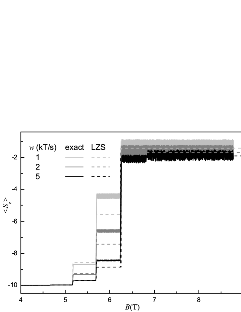
Figure 2: The expectation value of $\langle S_{z}\rangle$ (solid lines) as a function of the external magnetic field $B$ for different sweep rates. The exact results are compared with the predictions of the LZS approximation (dashed lines). The pulse shape corresponding to this figure is given by Eq. (10b). Above 5.7 T rapid oscillations appear, see the text for more details.

The initial state at the beginning of the calculation ($t=0$) is the lowest energy eigenstate that later crosses other adiabatic states, i.e., $\left|\Psi\right\rangle(0)=\left|E_{1}\right\rangle\approx|m=-10\rangle.$ This means that we follow the lowest increasing curve on the level scheme shown in Fig. 1, and the energy levels that cross this line correspond to decreasing energies and thus do not meet any other levels later. Similarly, if initially the ground state $|E_{0}\rangle$ was populated, it would not give any contribution to the steps in the magnetization curve, it simply leads, to a very good approximation, to an additional constant. (Which is the reason for our choice of the initial state.)

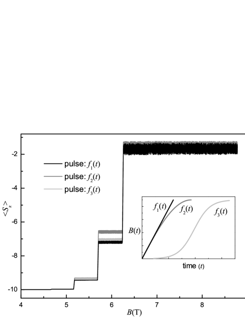
Figure 3: The expectation value of $\langle S_{z}\rangle$ as a function of the time dependent external magnetic field $B(t)$, which is shown in the inset, for three different pulse shapes with $w=2$ kT/s.

The expectation value $\langle S_{z}\rangle$ as a function of the external magnetic field $B$ is shown in Fig. 2 for the sine pulse (10b) and different values of the maximal sweep rate $w.$ The steps seen in this figure are very similar to the experimental curves, but differ from the result that can be obtained by using the LZS theory (also plotted in Fig. 2). Faster sweep rates mean smaller transition probabilities between the eigenstates of $S_{z}$. Although the exact dynamics is different from the LZS result, in the investigated sweep rate range we found that $\langle S_{z}\rangle$ scales with the sweep rate almost exactly the same way as one could deduce from $P_{LZS}$. Additionally, Fig. 2 also shows that since the states $|m\rangle$ are not exact eigenstates of the complete spin Hamiltonian $H_{S}$, there are rapid oscillations in $\langle S_{z}\rangle$ for higher external fields, which are clear indications of the Bohr oscillations corresponding to different eigenenergies of $H_{S}.$ We will find that if we take relaxation effects into account (Sec. IV), these oscillations disappear on a very short timescale.

Comparison between the results for $\langle S_{z}\rangle$ for different functional shapes of the external magnetic field $B(t)$ is shown in Fig. 3 in case of a maximal sweep rate of $w=2$ kT/s. Note that the difference is not too large; in this sweep rate range it is not the functional time-dependence of $B(t)$ that determines the heights of the steps seen in the magnetization curve, but rather its time derivative at the avoided level crossings. In other words, the approximation of a linearly increasing field $B$ around a certain transition point is sufficient to accurately describe the dynamics at that transition.

The population of the different eigenstates of $S_{z}$ and the adiabatic states $\left|E_{n}(t)\right\rangle$ are shown in Fig. 4 as a function of $B$ for the representative example of a pulse with linear shape and $w=1$ kT/s. As we can see, at the beginning of the time evolution, when the splitting of the adiabatic levels are very small and the magnetization is almost constant, the population of the $|m=-10\rangle$ state does not change significantly either. Around $B=5$ T the tunneling probability between different states $|m\rangle$ and $|m^{\prime}\rangle$ becomes appreciable, leading to the steps seen in Figs. 2 and 3. Note that the population of the adiabatic levels show an opposite behavior: initially practically all the population of the lower adiabatic level is transferred to the higher one at the avoided crossings. On the other hand, for larger external field values a nonzero population remains on the lower adiabatic level, leading to a noticeable change of the magnetization. The reason for the rapid oscillations in the populations of $|m\rangle$ seen in Figs. 2-4 is that at that high field strength $S_{z}$ and $H_{S}$ do not commute, therefore the states $|m\rangle$ are not exact eigenstates of the complete spin Hamiltonian. These oscillations disappear when we include relaxation, see Sec. IV.

If we restrict ourselves to the LZS model, then starting from the ground state it is sufficient to find the first value of $B$ at which this adiabatic level anticrosses the next one, calculate the LZS parameter $\Delta/\sqrt{\Omega}$ and use $P_{LZS}$ to obtain the population of the two relevant adiabatic levels after the transition, and repeat this process until the end of the time evolution. This approach includes the slow change of the levels $\left|E_{n}(t)\right\rangle,$ causing a slight, continuous increase of the magnetization as a function of $B$, but this effect is difficult to see in Figs. 2 and 3: the steps dominate the behavior of $\langle S_{z}\rangle.$ However, the LZS result obtained in this way is quantitatively different from the exact $\langle S_{z}\rangle(t)$ curve that was calculated by taking all the 21 levels into account (see Fig. 2). The position of the steps (determined by the avoided crossings) are the same, but their heights are different, and this difference can be as large as 30%.

In order to understand the physical reason for this effect, we have to investigate the relation between $P_{LZS}$ at a certain anticrossing and the relevant transition probability resulting from the present calculation.

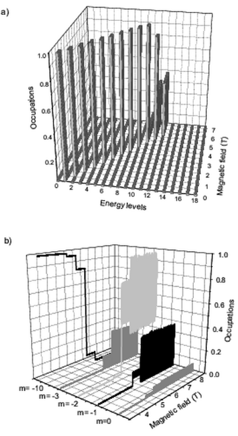
Figure 4: /Reduced resolution for this preprint version./ The population of the levels corresponding to the states $|E_{n}\rangle$ [a)] and $|m\rangle$ [b)] as a function of the external magnetic field for a linear pulse with $w=1$ kT/s. For the sake of simplicity in b) we show only populations larger than $0.05.$

The first important point to take into account is that, to a very good approximation, the transitions seen in Fig. 4 take place between two neighboring adiabatic levels. For sweep rates in the kT/s range the characteristic time of the transitionsVitanov (1999) at the avoided level crossings neither overlap nor influence each other. Let us now concentrate on a single step, as an example we focus on the vicinity of $B=5.7$ T (see Fig. 5), where the anticrossing levels $E_{11}$ and $E_{12}$ correspond to the states $\left|E_{11}\right\rangle\approx\left|m=-10\right\rangle$ ($\left|m=-1\right\rangle$) and $\left|E_{12}\right\rangle\approx\left|m=-1\right\rangle$ ($\left|m=-10\right\rangle$) before (after) the transition.

The most remarkable point concerning Fig. 5 is that it was obtained by assuming that only the adiabatic levels $\left|E_{11}\right\rangle$ and $\left|E_{12}\right\rangle$ play a role in the transition, the dynamics has been reduced to these two relevant levels. Calculating the same transition by taking all the 21 levels into account shows that this approximation estimates the exact dynamics with high accuracy. More generally, it is always possible to perform a similar reduction around a given avoided level crossing. Thus we obtain a method where a sequence of effective two-level transitions can describe the time evolution. The results obtained in this way are practically the same as those of the exact calculation, and considering the numerical costs, this is a very effective method.

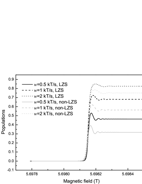
Figure 5: The population of the level $E_{11}$ around the transition $|E_{11}\rangle\rightarrow|E_{12}\rangle$ for different sweep rates. We compare the exact results with those from the LZS model. The external field pulse corresponding to this figure is given by Eq. (10a).

However, the time dependence of the expectation value of $\langle S_{z}\rangle$ obtained in this way is still different from the LZS result, despite the fact that the LZS theory is also based on a two-level approximation. Note that all the curves shown in Fig. 5 were calculated using the same numerical method, the pulse shape ($f_{1}$), the initial state and the level splitting were also the same for all the calculated sweep rates: the only difference was the time dependence of the energy levels and their coupling. (In fact, as it is clear from Eqs. (6), (7) and (8), it is only the energy difference $E_{12}(t)-E_{11}(t)$ that plays a role here.) These are multilevel effects: the time dependence of the $2\times 2$ Hamiltonian obtained by the reduction of $H_{S}$ to the relevant level pair is affected by all the other levels, similarly to a renormalization effect. The influence of the states not taking part in the transition results in a time dependence of the parameters of the reduced Hamiltonian which is slightly different from the LZS model described by Eq. (9). That is, the single parameter $\Delta/\sqrt{\Omega}$ is not enough to describe these transitions, or in other words, we have time dependent factors in the LZS matrix elements $\Delta(t),\Omega(t).$ That is emphasized by calculating the long time limit transition probability for the same transition shown in Fig. 5 with different parameters in the Hamiltonian (3) in such a way, that the sweep rate and the level splitting are fixed. As an example, we consider the level splitting $\Delta$ at this transition as a function of only two parameters, namely $C$ and $K$; we do not change $D,F$ and $E$ in $H_{S}.$ First we calculate $\Delta(C,K)$ using the parameters given in Sec. II and obtain $\Delta_{0}=1.47\times 10^{-4}$ (in Kelvin). Then we solve the equation $\Delta(C,K)=\Delta_{0}$ to find the parameter pairs $\{C,K\}$ that correspond to the same level splitting as it was initially. It turns out that there are several disconnected lines in the $C-K$ plane along which $\Delta(C,K)=\Delta_{0}$, and consequently $P_{LZS}$ is constant for a given sweep rate. But as we can see in Fig. 6, the calculated non-LZS transition probabilities, long after the transition took place, strongly depend on the parameter $C$ in Eq. (3): they range from 5% up to 65%, and can be both higher and lower than $P_{LZS}$. Different symbols in Fig. 6 correspond to different lines along which $\Delta(C,K)=\Delta_{0}$. In any case, we can conclude that the final transition probability at a given avoided crossing is also influenced by the levels that do not take part in the relevant transition, and can therefore not be described within the framework of the LZS model.

Figure 6: The final population of the level $E_{11}$ after the transition $|E_{11}\rangle\rightarrow|E_{12}\rangle$ around $B=5.7$ T as a function of the parameter $C$ in Eq. (3). The level splitting $\min(E_{12}-E_{11})$ is kept fixed, leading to the constant final population in the LZS model indicated by the solid horizontal line. The magnetic field pulse used is given by Eq. (10a) with $w=1$ kT/s.

IV Relaxation effects

So far we considered unitary time evolution, i.e., the Hamiltonian (1) governed the dynamics. However, there are interactions with e.g. phonons that are not included in $H_{S}.$ These additional degrees of freedom can be considered as the environment of the spin system, and any realistic description should take their influence into account.Leuenberger and Loss (2000); Rousochatzakis and Luban (2005); Benedict et al. (2005) Additionally, as we shall see in this section, the rapid oscillations seen in Figs. 2-4 disappear on a very short time scale when relaxation influences the dynamics.

Since phase relaxation is usually much faster than energy exchange between the investigated quantum system and its environment, we concentrate on this kind of decoherence, and assume a Lindblad-typeLindblad (1976) dynamical equation:

$$\frac{\partial\varrho}{\partial t}=-i\left[H_{S},\varrho\right]+\frac{\gamma}{2}\left(2S_{z}\varrho S_{z}-S_{z}^{2}\varrho-\varrho S_{z}^{2}\right).$$ (11)

The second term in this master equation will not change either the magnetization of the sample nor the expectation value of $H_{0}$. It leads to the gradual disappearance of the non-diagonal elements of $\varrho$ in the eigenbasis of $S_{z}$ without changing the populations $\varrho_{nn}.$ The result of this kind of relaxation is quite different during the transitions at the avoided level crossings and between them. This difference is clearly seen if we consider sweep rates of the order of kT/s, when the characteristic transition times are $10^{-6}$–$10^{-7}$ s, while the spin system spends about $10^{-3}$ s between two level crossings. These time scales should be compared to $\gamma^{-1},$ which is in the range of $10^{-5}$–$10^{-7}$ s for low temperatures ($T\approx 2K$) at which several experiments were performed. Thus, between two crossings, relaxation has enough time to destroy the phase information almost completely.

Figure 7: The effect of phase relaxation on the dynamics of the magnetization ($\langle S_{z}\rangle$) around the transition $|E_{11}\rangle\rightarrow|E_{12}\rangle.$ We assumed a linear pulse given by Eq. (10a) with maximal sweep rate $w=1$ kT/s in part a) and $2$ kT/s in part b). Note that the origin of the time axis has been shifted, $t=0$ corresponds to the time when $E_{12}-E_{11}$ is minimal.

In other words, if after an avoided crossing the system is in a pure quantum mechanical state $|\phi\rangle$, the initial condition at the next crossing can be considered as the right hand side of the following scheme:

$$\left|\phi\right\rangle\left\langle\phi\right|=\sum_{nm}\left|n\right\rangle\left\langle m\right|\varrho_{nm}\ \rightarrow\ \sum_{m}\left|m\right\rangle\left\langle m\right|\varrho_{mm}.$$ (12)

Note that the Hamiltonian part of the time evolution slightly modifies the process above, but the final consequence, i.e., that dephasing changes the initial conditions for the transitions at the avoided level crossings is still valid. Decoherence as described by Eq. (12) plays an important role in the physical mechanism responsible for the observed form of hysteresis loops (see Ref. [Vogelsberger and Garanin, 2006] for experimental results on systems of low-spin magnetic molecules). We found that even for such fast external magnetic field sweep rates as a few kT/s, quantum mechanical interference does not play an important role in transitions at consecutive anticrossings, by the time the system reaches the next transition point, the phase information has already flown into the environment. For similar reasons the formation of closed hysteresis curves cannot be influenced either by quantum interference. However, even faster sweep rates, or faster return to a certain transition by superimposing an oscillating magnetic field on a constant one around a certain crossing, may give rise to quantum mechanical interference effects. We predict that such interference phenomena will show up for magnetic field sweep rates in the MT/s range. They will be seen as a very strong dependence of the form of the hysteresis loops on the sweep rate due to the extreme sensitivity of the process to the relative phases of the states that take part in a transition.

The phenomena expected around transition regions are more interesting, as they are consequences of the interplay between coherent effects and dephasing: the characteristic time of the transitions are comparable, but usually shorter than the dephasing time defined by $\gamma^{-1}.$ The general consequence of the second term in the master equation (11) is that it decreases the transition probability in the $\{|m\rangle\}$ basis, i.e., when relaxation is present, it makes the steps in the magnetization smaller (see Fig. 7). The larger the value of $\gamma$, the stronger this effects is, which underlines again the importance of the relative phase in this physical system. In the previous section it was shown that phases gained by the adiabatic states at an anticrossing can remarkably modify the transition probability, now we see that loss in phase information has also strong effects. Note that in contrast with the coherent case (see Sec. III), the final transition probabilities in the presence of dephasing do not scale with the sweep rate similarly to the LZS case. For larger sweep rates the system spends less time in the transition region, and consequently decoherence less strongly modifies the final transition probability. That is, the larger the magnetic field sweep rate, the more similar the dynamics around a transition becomes to the case without dephasing. Additionally, we want to point out that the coherent oscillations, the consequences of which has been seen in Figs. 2-4, are strongly damped even for weak dephasing.

However, the statement that the final transition probabilities are modified by the presence of all the levels and thus cannot be accurately described within the framework of a LZS model (even if we include relaxation as well) is also true in the present case. Additionally, let us emphasize that the parameter region discussed here is different from the strongly damped one studied in Refs. [Leuenberger and Loss, 1999, 2000], where incoherent tunneling can give a proper description. For external field sweep rates in the kT/s range, neither coherent time evolution nor relaxation dominates, which leads to an interesting interplay between these two qualitatively different processes.

V Conclusions

We studied the time evolution of the spin degrees of freedom in molecular nanomagnets, with a focus on the molecule Mn₁₂-Ac in the presence of time-dependent magnetic field. Using an appropriate ’exact numerical’ method, we followed the time evolution from zero external magnetic field until saturation of the magnetization is reached. We found that for sweep rates in the kT/s range, steps in the magnetization originate from two-level transitions which cannot be described within the framework of the Landau-Zener-Stückelberg (LZS) model. This observation led us to the introduction an efficient and accurate approximation based on two-level non-LZS transitions. This method introduces the possibility of performing long term dynamical calculations that can directly be related to experiments. We also demonstrated that the sweep rate range of kT/s is special in the sense that for realistic relaxation times, there are observable consequences of the competition between coherent dynamics and decoherence that modify the heights and widths of the magnetization steps.