The Goldstone mode of planar optical parametric oscillators

Abstract

We propose an experimental setup to probe the low-lying excitation modes of a parametrically oscillating planar cavity, in particular the soft Goldstone mode which appears as a consequence of the spontaneously broken $U(1)$ symmetry of signal/idler phase rotations. Differently from the case of thermodynamical equilibrium, the Goldstone mode of such a driven-dissipative system is an overdamped mode, whose linewidth goes to zero in the long-wavelength limit. When the phase of the signal/idler emission is pinned by an additional laser beam in the vicinity of the signal emission, the $U(1)$ symmetry is explicitely broken and a gap opens in the Goldstone mode dispersion. This results in a dramatic broadening of the response to the probe. Quantitative predictions are given for the case of semiconductor planar cavities in the strong exciton-photon coupling regime.

I Introduction

A central concept of the modern theory of phase transitions in systems at thermodynamical equilibrium is the so-called Goldstone mode, which appears as a consequence of the spontaneous breaking of a continuous symmetry goldstone-stat-mech . Unless the system has long-range interactions anderson , this mode has the general property of being a soft mode, whose frequency dispersion $\omega_{G}(k)$ tends to zero in the long-wavelength limit $k\rightarrow 0$. The Goldstone mode corresponds in fact to a spatially slow twist of the order parameter, whose energy cost tends to zero in the long-wavelength limit. Among the most celebrated examples of Goldstone modes in condensed matter physics we can mention the zero-sound mode of superfluid Helium 4 or dilute Bose-Einstein condensates and the magnon excitations in ferromagnets. Zero-sound is related to the spontaneous breaking of the $U(1)$ gauge symmetry of the quantum Bose field below the Bose-Einstein condensation temperature goldstone-stat-mech ; forster ; pines-nozieres , while the magnon branch is related to the spontaneous breaking of the rotational symmetry of the magnetic moment orientation below the Curie temperature magnon .

The concept of a Goldstone mode plays an important role also in the physics of nonlinear dynamical systems far from thermodynamical equilibrium cross , whose stationary state is not determined by a thermodynamical equilibrium condition, but is rather the result of a dynamical equilibrium between an external driving force and the dissipation. In many examples of such driven-dissipative systems a homogeneous state develops a non-trivial spatiotemporal pattern when the driving force exceeds a critical value. The most famous example of this pattern formation behaviour is perhaps the regular periodic arrangement of Bénard cells that appears in heat convection through a viscous fluid when a sufficiently large temperature gradient (driving force) is applied in the vertical direction so to exceed the braking effect of viscosity (dissipation) benard . The continuous translational symmetry of the initially homogeneous system is reduced to the discrete symmetry of the periodic pattern of Bénard cells. As a consequence of the spontaneously broken symmetry, a neutral mode of vanishing frequency and damping rate appears in the linear stability analysis around the stationary state of the system, a mode which corresponds to the rigid translation of the whole roll pattern in space. This neutral mode is the non-equilibrium counterpart of the Goldstone mode of equilibrium statistical mechanics.

Another well celebrated example of pattern formation takes place in optical parametric oscillation (OPO) in planar cavities OPO_exp . Differently from the more usual case of spherical mirror cavities with a discrete and well-spaced set of modes, planar cavities dispose of a continuum of modes in which the parametric emission can take place, so that the light field has a rich spatial dynamics planar_OPO_2 . In the OPO state, a periodic spatial pattern is indeed created in the cavity plane by interference of the pump, signal and idler fields. In addition to their interest from the point of view of fundamental physics, technological applications of planar OPOs have also been actively investigated in view of using them as flexible light sources in new frequency ranges, or even as sources of entangled photons for quantum cryptography quantum_crypt .

In recent years, a great deal of theoretical and experimental activity has concerned planar semiconductor microcavities with quantum well excitonic transitions strongly coupled to the cavity mode review1 ; review2 . At linear regime, the elementary excitations of these systems are cavity-polaritons, i.e. a superposition of a cavity photon and a quantum well exciton. Cavity-polaritons have the interesting property of combining the extremely strong Kerr nonlinearity due to the excitonic component to a peculiar dispersion relation which allows for easy and robust phase-matching of the optical parametric process. In this way, large values of gain have been observed in parametric amplification OPA_mcav , as well as parametric oscillation at low pump intensity values stevenson ; houdre . Extensive studies of the parametric oscillation process in semiconductor planar microcavities have verified the coherent nature of the parametric emission above threshold by observing a frequency narrowing of the emission stevenson , the absence of dispersion houdre , as well as the long-range spatial coherence baas-coh .

As it happened for atomic Bose-Einstein condensates book , a good deal of information on the state of the polariton system can be obtained by looking at the elementary excitations of the system around its dynamical equilibrium state. The elementary excitations around the pump-only state below the threshold for parametric oscillation have been theoretically investigated in superfl , and predictions have been put forward for polariton superfluidity effects. In the present paper, we shall investigate the elementary excitation spectrum around the parametric oscillation steady state above threshold. Since a continuous $U(1)$ symmetry related to the signal/idler phases is spontaneously broken, a Goldstone mode has to appear in the excitation spectrum of the planar system, whose frequency and damping rates go to zero in the $k\rightarrow 0$ long-wavelength limit. Although its existence has been recently mentioned zambrini and its role in the destruction of long-range coherence in 1D systems discussed zambrini ; coherence , no experiments have been so far performed nor proposed which are able to directly observe the Goldstone mode of optical parametric oscillators. Pioneering work on the elementary excitation spectrum around a parametrically oscillating state was reported in Ref.ciuti-offbranch both in the presence of a laser beam driving the signal mode, and in a pump-only configuration. The emission was experimentally observed and its spectrum compared to a calculation of the elementary excitation dispersion. However, no specific attention was paid in the experiment to the region where the Goldstone mode is expected to appear, nor any mention made to it in the theoretical analysis. The same with other recent theoretical papers that address the excitation spectrum around a parametrically oscillating state of a semiconductor microcavity savona ; whittaker2 .

The main point of the present paper is to give a complete account of the physics of the Goldstone mode of a planar optical parametric oscillator above threshold, and to propose a way of probing it with an additional laser beam. In Sec.II we present the physical system and the theoretical framework used for its description. In Sec.III we study the stationary state of parametric oscillation above threshold and we introduce the concept of spontaneous breaking of the $U(1)$ signal/idler phase symmetry. The spectrum of the elementary excitations around the stationary state is calculated and discussed in the following Sec.IV, and then used to evaluate the linear response of the system to a weak probe beam at angles close to the signal emission: the Goldstone mode is shown to give a strong and narrow peak at low frequencies, whose linewidth tends to zero as the direction of the probe beam is brought closer to the signal emission one. The consequences of the presence of an additional signal laser field at exactly the same wavevector as the signal emission are investigated in Sec. V. From the full equations of motion, one finds that the phase of the signal emission results in this case pinned to the one of the signal beam so that the $U(1)$ symmetry is explicitely broken. No Goldstone mode is therefore present any longer and a gap opens up in the dispersion of the elementary excitations. As a consequence, a dramatic broadening of the peak corresponding to the Goldstone mode is observed in the response spectrum to the probe. This phenomenology is the non-equilibrium analog to what happens in a ferromagnet when an external magnetic field is applied to the system to break the rotational symmetry. In this case, the orientation of the magnetization is fixed by the applied field and a gap opens up in the magnon dispersion magnon .

The two last section are devoted to the analysis of issues of experimental relevance. The consequences of a possible frequency mismatch of the applied signal beam from the natural frequency of the signal emission are investigated in Sec. VI, while the effect of the spatial inhomogeneities due to the finite pump spot are addressed in Sec.VII. Both these issues are shown not to affect the properties of the Goldstone mode discussed in the previous sections. Conclusions are drawn in Sec.VIII. Three appendices are devoted to a brief summary of the analytical equations definining the stationary state of the homogeneous system, to the analytical properties of the Goldstone mode frequency around $k=0$, and to the comparison with the case of OPOs based on a $\chi^{(2)}$ second-order nonlinearity.

II Physical system and theoretical model

The physical system we are considering consists of a planar semiconductor microcavity containing a quantum well with an excitonic transition strongly coupled to the cavity mode. A sketch is shown in Fig.1. The elementary excitations of this system are cavity-polaritons, i.e. coherent superpositions of cavity photons and excitons, which satisfy the Bose statistics. The photonic component is essential to couple to the external incident radiation, while the excitonic component provides the exciton-exciton collisional interactions which are responsible for the parametric process.

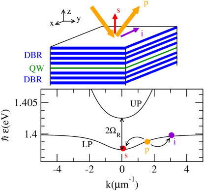
Figure 1: Upper panel: sketch of the microcavity system and the parametric process under consideration. Lower panel: Lower polariton (LP) and upper polariton (UP) dispersion. The cavity photon dispersion is $\omega_{C}(k)=\omega_{C}^{0}\,\sqrt{1+{k^{2}}/{k_{z}^{2}}}$ with $\hbar\omega^{0}_{C}=1.4$ eV and $k_{z}=20\,\mu\rm m^{-1}$. The exciton dispersion is flat and resonant with the $k=0$ cavity mode $\omega_{X}=\omega_{C}^{0}$. The exciton-photon Rabi coupling is $\hbar\Omega_{R}=2.5$ meV. Dots indicate the signal, pump and idler modes.

Given the translational invariance of the system along the cavity plane, the in-plane wave vector ${\mathbf{k}}$ is a good quantum number and the polaritonic dispersion can be studied as a function of ${\mathbf{k}}$. As shown in Fig.1b, two polaritonic branches exist in the polariton spectrum, split by twice the Rabi frequency $\Omega_{R}$ of the exciton-photon coupling review1 ; review2 . A simple, but so far accurate model for interactions is based on a repulsive exciton-exciton two-body contact interaction of strength $g$.

In the following we will focus our attention on the lower polariton branch only, which is more protected from loss and decoherence processes. Its dispersion will be denoted as $\epsilon(k)$. In order to justify the neglection of the upper polariton, one has to check that the Rabi splitting $\Omega_{R}$ is much larger than both the detuning of the incident laser (of frequency $\omega_{p}$ and wave vector $k_{p}$), and the nonlinear shift $\epsilon_{mf}\lesssim g\,n_{LP}$ of the polariton mode ($n_{LP}$ is here the polariton density). These condition are actually well satisfied in current experiments.

At the mean-field level, the dynamics of the polaritonic field can be described by a polaritonic Gross-Pitaevskii equation ciuti_review ; superfl , whose $k$-space form reads:

$$i\frac{d}{dt}\psi_{LP}(k)=\left[\epsilon(k)-i\frac{\gamma}{2}\right]\psi_{LP}(k)+F_{p}(k)\,\,e^{-i\omega_{p}t}\\ +\sum_{q_{1},q_{2}}g_{k,q_{1},q_{2}}\,\psi^{*}_{LP}(q_{1}+q_{2}-k)\,\psi_{LP}(q_{1})\,\psi_{LP}(q_{2}).$$ (1)

$F_{p}(k)$ is here the amplitude of the incident pump laser field, which is assumed to be continuous wave and monochromatic at $\omega_{p}$. Unless otherwise specified (as e.g. in Sec.VII), a plane-wave at $k_{p}$ is taken for its spatial profile $F_{p}(k)=F_{p}\delta_{k,k_{p}}$. The damping rate $\gamma$ is the sum of the contribution of radiative and non-radiative losses. It has been taken for simplicity as momentum-independent. The momentum-dependent nonlinear interaction strength for polaritons $g_{k,q_{1},q_{2}}$ is defined in terms of the Hopfield coefficient $U_{X}$ quantifying the excitonic content of the polariton ciuti_review as:

$$g_{k,q_{1},q_{2}}=g\,U^{*}_{X}(k)\,U^{*}_{X}(q_{1}+q_{2}-k)\,U_{X}(q_{1})\,U_{X}(q_{2}),$$ (2)

Note that the same equation (1) can be used to describe the photon dynamics in different systems, e.g. metallic mirror planar cavities containing a Kerr nonlinear medium butcher . In this case, no excitonic field is present and the polaritonic field ${\hat{\Psi}}_{LP}$ reduces to the bare e.m. field ${\hat{E}}$. The nonlinear coupling constant $g$ is then provided by the Kerr optical nonlinearity of the cavity material (of dielectric constant $\epsilon_{\rm lin}$ and thickness $d$), and is proportional to its third-order nonlinear polarizability $\chi^{(3)}$:

$$\hbar g=C\chi^{(3)}(\hbar\omega_{0})^{2}/(d\epsilon_{\rm lin}^{2}),$$ (3)

where $C$ is a numerical factor of order one that takes into account the boundary conditions at the cavity mirrors.

Quantitatively, one however should keep in mind that the nonlinear coupling constant $g$ for semiconductor microcavities in the strong exciton-photon coupling regime $\hbar g\approx 5\times 10^{-6}\,\textrm{eV}\,\mu\textrm{m}^{2}$ is orders of magnitude larger than the one that is obtained in standard transparent media for nonlinear optics. Organic materials specifically suited for nonlinear optical applications have in fact $\chi^{(3)}$ up to about $10^{-9}\,\textrm{erg}^{-1}\,\textrm{cm}^{3}$ cont-nonlin-opt , which yields values for the nonlinear coupling constant of the order of $\hbar g=5\times 10^{-9}\,\textrm{eV}\,\mu\textrm{m}^{2}$. Conventional inorganic materials have even weaker susceptibilities.

III Parametric oscillation and spontaneous symmetry breaking

Among the many processes described by the motion equation (1) in the different regimes, the focus of the present paper will be concentrated on parametric process in which two polaritons in the pump mode (wave vector $k_{p}$ and frequency $\omega_{p}$) collide and are converted into a pair of signal and idler polaritons, of wave vectors respectively $k_{s}$ and $k_{i}=2k_{p}-k_{s}$ and frequencies $\omega_{s}$ and $\omega_{i}=2\omega_{p}-\omega_{s}$. As shown in Fig.1, the peculiar polaritonic dispersion allows for the parametric process to occur in a triply-resonant way, i.e. with all the $\omega_{p,s,i}$ close to resonance with the free polariton energy $\epsilon(k_{p,s,i})$. Such a process is described by a term in the nonlinear interaction Hamiltonian of the form:

$$H_{\rm int}=g_{k_{p},k_{s},k_{i}}\,\Big{[}{\hat{\Psi}}^{\dagger}_{LP}(k_{p})\,{\hat{\Psi}}^{\dagger}_{LP}(k_{p})\,{\hat{\Psi}}_{LP}(k_{i})\,{\hat{\Psi}}_{LP}(k_{s})+\\ +{\textrm{h}.c.}\Big{]},$$ (4)

where ${\hat{\Psi}}_{LP}$ is the polariton quantum field operator.

It is important to remind that OPO operation can also make use of a different nonlinear process, in which a single pump photon is split into a pair of signal/idler photons. The nonlinear susceptibility involved in this parametric downconversion process is the second-order one $\chi^{(2)}$. Before the advent of semiconductor microcavities in the strong coupling regime, most of the existing literature on OPOs was indeed based on such parametric down conversion processes planar_OPO_2 . Although our attention will be in the following concentrated on the specific case of semiconductor microcavities, the concept of the Goldstone mode extends without almost any change to the other case. A brief discussion of these issues is given in Appendix C.

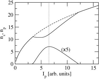
Figure 2: Pump and signal intensity as a function of the pump power for $k_{s}=0.075\mu\rm m^{-1}$. Pump parameters $k_{p}=1.57\mu\rm m^{-1}$ and $\omega_{p}=1.39875$. Cavity and exciton parameters correspond to the LP dispersion shown in figure 1b.

In order to study the parametric process the following ansatz can be used for $\psi_{LP}(x,t)$:

$$\psi_{LP}(x,t)=P\,e^{i(k_{p}x-\omega_{p}t)}+S\,e^{i(k_{s}x-\omega_{s}t)}+\\ +I\,e^{i(k_{i}x-\omega_{i}t)},$$ (5)

where $k_{s}$ is considered here as a given parameter. A detailed analysis of its behaviour as a function of the geometry and system parameters is postponed to a forthcoming publication pattern .

This ansatz allows for finite amplitudes $P,S,I$ in respectively the pump, signal and idler modes, while all other modes are assumed to remain empty. The possible occupation of other modes via multiple scattering processes, as observed in ciuti-offbranch ; tarta is therefore not taken into account by our model. This approximation is well justified by the fact that the (small) polariton population in these modes does not affect the physics under examination but can only give quantitatively small corrections. The values of $P,S,I$ in the stationary state, as well as the parametric oscillation frequency $\omega_{s}$ are obtained by inserting this ansatz in the equation of motion (1). Details of the equations are given in Appendix A.

The pump and signal intensities in the stationary state are plotted in Fig.2 as a function of the pump intensity $I_{p}=|F_{p}|^{2}$ for a pump frequency $\omega_{p}<\epsilon(k_{p})$, in which case the pump-only dynamics corresponds to optical limiting superfl . The main feature is the onset of parametric oscillation for pump intensities $I_{p}$ within a certain range of values. Outside this range, the pump-only solution $S=I=0$ remains a dynamically stable solution of the mean-field dynamics.

While the amplitude $P$ of the pump mode is completely determined (both in modulus and in phase) by the incident laser amplitude, the signal and idler phases remain free thanks to the invariance of the equation of motion (1) and of the Hamiltonian (4) under a simultaneous phase rotation of the signal and idler in opposite directions:

$$S\rightarrow S\,e^{i\Delta\phi}\hskip 28.45274ptI\rightarrow I\,e^{-i\Delta\phi}.$$ (6)

In the parametrically oscillating state, $S$ and $I$ have a non-vanishing value, so that this $U(1)$ phase-rotation symmetry is spontaneously broken. In the absence of external perturbations, the specific value of the phase of $S$ (and consequently of $I$) is randomly selected at each realization of the experiment. Consequences of the underlying symmetry are however present: no restoring force opposes a simultaneous and opposite rotation of the signal and idler phases, which then slowly diffuse in time under the effect of fluctuations phase_diffusion . In the next section, we shall show how the spontaneosly broken symmetry manifests itself as a strong response of the system when spatial twists of the signal/idler phases are created by an extra probe laser at frequency $\omega_{r}=\omega_{s}+\Delta\omega$ and wavevector $k_{r}=k_{s}+\Delta k$ close to the frequency and wavevector of the signal emission $|\Delta k|\ll|k_{s}-k_{p}|$.

IV Response to a weak perturbation and the Goldstone mode

Provided the applied perturbation is weak, the response of the polariton field can be calculated by linearising the mean-field equations of motion around the solution (5). Modifying this solution as

$$S \rightarrow S+u_{s}\,e^{i(\Delta k\,x-\Delta\omega\,t)}+v^{*}_{s}\,e^{-i(\Delta k\,x-\Delta\omega\,t)}$$ (7)

$$P \rightarrow P+u_{p}\,e^{i(\Delta k\,x-\Delta\omega\,t)}+v^{*}_{p}\,e^{-i(\Delta k\,x-\Delta\omega\,t)}$$ (8)

$$I \rightarrow I+u_{i}\,e^{i(\Delta k\,x-\Delta\omega\,t)}+v^{*}_{i}\,e^{-i(\Delta k\,x-\Delta\omega\,t)},$$ (9)

the deviations from the steady state can be grouped in a 6-vector $\mathcal{U}=(u_{s},u_{p},u_{i},v_{s},v_{p},v_{i})^{T}$ that obeys the equation

$$\Delta\omega\,{\mathcal{U}}-{\mathcal{L}}(\Delta k)\,{\mathcal{U}}={\mathcal{F}}_{r}$$ (10)

with a force vector which for our specific excitation scheme reads $\mathcal{F}_{r}=(F_{r},0,\ldots,0)^{T}$. The observable quantity is the number of polaritons created in the $k_{r}$ mode, which corresponds to the square modulus of the first element $u_{s}$ of the system response ${\mathcal{U}}$.

The matrix $\mathcal{L}$ has the typical Bogoliubov structure

$$\mathcal{L}(\Delta k)=\left(\begin{array}[]{cc}M(\Delta k)&Q(\Delta k)\\ -Q^{\ast}(\Delta k)&-M^{*}(-\Delta k)\end{array}\right),$$ (11)

where the $3\times 3$ matrices $M(k)$ and $Q(k)$ are defined as:

$$M_{mn}(k) = [\varepsilon(k_{m}+k)-\omega_{m}-i\gamma/2]\,\delta_{m,n}$$ (12)

$$+ 2\sum_{rt=1}^{3}\,g_{k_{m}+k,k_{n}+k,k_{t}}\delta_{m,n+r-t}A^{*}_{r}A_{t}$$

$$Q_{mn}(k) = \sum_{rt=1}^{3}g_{k_{m}+k,k_{r},k_{s}}\delta_{m+n,r+t}\,A_{r}A_{s}.$$ (13)

Here we have identified the three modes $s,p,i$ with respectively the values $1,2,3$ of the matrix and vector indices, so that e.g. $A_{1}=S$, $A_{2}=P$ and $A_{3}=I$.

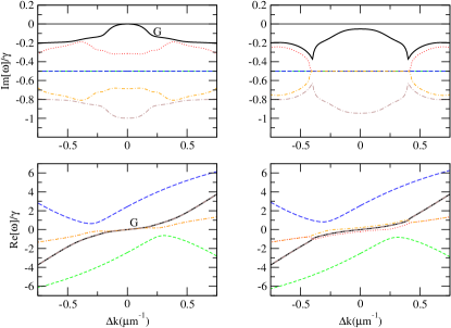
Figure 3: Imaginary (upper panels) and real (lower panels) part of the excitation spectrum around the stationary state for the pump intensity corresponding to the dashed line in fig.2. The left panels refer to the case in which the signal/idler phase rotation symmetry is spontaneously broken and a Goldstone mode $G$ is present (heavy line). The right panels refer to the case where a small signal laser beam ($I_{s}/I_{p}=0.0023$) is present to explicitely break this symmetry and destroy the Goldstone mode. Cavity and pump parameters as in figure 2

The real and imaginary parts of the eigenvalues of the Bogoliubov matrix $\mathcal{L}(\Delta k)$ give respectively the frequency and linewidths of the elementary excitations around the parametrically oscillating stationary state. These fix the shape of the luminescence peaks as observed e.g. in the experiment of ciuti-offbranch , as well as the poles of the response to the probe beam. A typical example of this Bogoliubov dispersion as a function of $\Delta k$ is plotted in the left panels of Fig. 3: the most relevant feature is the presence of a branch of eigenvalues $\omega_{G}(\Delta k$) tending to exactly zero for $\Delta k\rightarrow 0$.

The presence of this branch is a direct consequence of the fact that the mean field steady state (5) spontaneously breaks the $U(1)$ symmetry of the signal/idler phase: as any global phase rotation of $S,I$ of the form (6) maps a stationary state of (1) into another stationary state with different signal/idler phases, the generator $G^{T}=(iS,0,-iI,-iS^{*},0,iI^{*})$ of the signal/idler phase rotations is an eigenvector of the matrix ${\mathcal{L}}(\Delta k=0)$ with zero eigenvalue $\omega_{G}(\Delta k=0)=0$. For finite values of $\Delta k$, the soft Goldstone branch at $\omega_{G}(\Delta k)$ corresponds to a spatially varying twist of the signal/idler phases.

The existence of a soft Goldstone mode is a general result valid for both non-equilibrium cross and equilibrium goldstone-stat-mech systems: in this latter case, the Goldstone mode corresponds to the magnon mode of ferromagnets magnon , or to the zero sound mode in superfluid liquid Helium and Bose-Einstein condensates forster ; pines-nozieres .

Fundamental differences however exist, which make the physics of the two cases quite distinct. In Bose systems at equilibrium, the dispersion of the Golstone mode goes as $\textrm{Re}[\omega(k)]\simeq c_{s}\,|k|$ around $k=0$ and shows a singularity at $k=0$. This branch corresponds to weakly damped sound waves which in the long-wavelength limit propagate at the speed of sound $c_{s}$.

In the present non-equilibrium case, no singularity appears in the dispersion relation $\omega_{G}(\Delta k)$ of the Goldstone mode. In particular, the real part $\textrm{Re}[\omega(\Delta k)]\propto\Delta k$ has a continuous and non-vanishing slope at $\Delta k=0$. This fact is due to the flow of the pump polaritons which are injected with a finite wave vector $k_{p}$ and are able to drag the elementary excitations. On the other hand, convective stability and analyticity arguments (see Appendix B) show that the imaginary part goes as $\textrm{Im}[\omega(\Delta k)]\approx-\alpha\,(\Delta k)^{2}$ for small $\Delta k$ with a positive $\alpha>0$.

Combining these facts together, one can physically summarize that the Goldstone mode of a planar OPO consists of a spatially slowly varying twist of the signal and idler phases, which however does not propagate as a sound wave, but has a diffusive character. Once a localized perturbation is created in the system, this will simply relax back to the equilibrium state while it is dragged by the pump polariton flow. This overdamped character is a remarkable difference with respect to the equilibrium case.

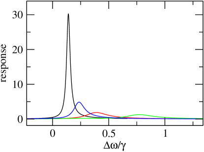
Figure 4: Response spectrum to a probe beam for several values of the wavevector $\Delta k=k_{r}-k_{s}=0.1,\,0.15,\,0.2,\,0.3\,\mu\textrm{m}^{-1}$ (black, blue, red, green). Cavity and pump parameters are the same as in figure 2.

The general properties of the eigenvalues of the Bogoliubov matrix (11) can be used to physically understand the response spectra shown in Fig.4: the number of polaritons created by the probe in the $k_{r}=k_{s}+\Delta k$ mode is here plotted as a function of its frequency $\omega_{r}=\omega_{s}+\Delta\omega$. The most apparent feature is the strong and narrow peak that appears at low frequencies for a probe wavevector $k_{r}$ close to the signal one $k_{s}$. In particular, its linewidth can be much smaller than the damping rate $\gamma$ of the polariton mode: as $k_{r}$ approaches $k_{s}$, the linewidth goes to $0$ and the peak height diverges, while the peak dramatically broadens for increasing $\Delta k$. Comparing these spectra with the dispersion of the elementary excitations shown in Fig.3, one can immediately see that the strong peak corresponds to the pole at $\omega_{G}(\Delta k)$, and therefore to the excitation of the soft Goldstone mode.

An experimental observation of this narrow peak in the probe response spectra with the characteristic dependence on the probe angle would provide a unambiguous signature of the Golstone mode. In our previous work coherence , the excitation of the Goldstone mode by the quantum fluctuations showed up as a $k$-space broadening of the signal emission in the absence of any probe. Although this broadening of the luminescence pattern is of conceptual interest from the point of view of low-dimensional non-equilibrium physics, the pump-probe experiment discussed here appears as more favourable in view of the experimental observation of the Goldstone mode. The response to the probe can be measured by comparing pairs of spectra taken respectively in the presence and in the absence of the probe, so to subtract out the background of signal light scattered by the defects of the sample.

V Destroying the Goldstone Mode

It is a well-known fact that the rotational symmetry can be explicitely broken in a ferromagnet by adding an external magnetic field that fixes a preferential orientation for the magnetization and therefore opens a gap in the magnon dispersion magnon . While a pinning of the Bose field phase is hardly obtained in Helium or atomic Bose-Einstein condensates because of particle number conservation goldstone-stat-mech , it can be easily done in the optical experiment proposed here by applying an extra laser beam (called hereafter signal laser) at exactly the signal frequency $\omega_{s}$ and wave vector $k_{s}$ . In this way, stimulated processes push the parametric emission to preferentially occur with a phase pinned to the incident signal laser one. This pinning of the signal field phase is the parametric and multi-mode analog of what happens in a single-mode laser when a coherent signal is injected in the cavity degiorgio ; scully . In the pattern formation literature, the idea of forcing a specific pattern shape by means of an additional beam often goes under the name of pattern synchronization. First studies of such issues in an optical context have recently appeared using a completely different setup Neubecker .

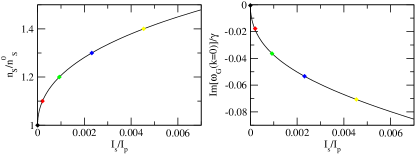
Figure 5: Signal mode occupation (left panel) and amplitude of the gap $\textrm{Im}[\omega_{G}(\Delta k=0)]$ (right panel) as a function of the signal laser power $I_{s}$. The coloured points mark the $I_{s}$ values of the spectra in Fig.6.

As the Goldstone mode has a pole at exactly the signal laser frequency and wavevector, the change of $S$ due to the application of the signal beam cannot be calculated by means of the linearized theory, but has to be calculated including he signal laser beam as an additional term in the full equation of motion (1), as shown in Appendix A.

The left panel of Fig. 5 shows the signal amplitude as a function of the signal laser amplitude: for small values of $I_{s}$, the signal intensity $|S|^{2}$ shows a square root behaviour as a function of $I_{s}$. As $S$ is an analytic function of $F_{s}$, one can expand $S\simeq S_{0}+cF_{s}$, the square modulus of which immediately gives the square-root behaviour $|S|^{2}-|S_{0}|^{2}\simeq c\,|S_{0}|\,|F_{s}|\propto\sqrt{I_{s}}$.

The effect of the signal laser on the Bogoliubov dispersion is shown in the right panels of of Fig. 3: the imaginary part $\textrm{Im}[\omega_{G}(\Delta k)]$ shows now a finite gap at $\Delta k=0$, so that no Goldstone mode exist any longer. The damping rate of Bogoliubov excitations is finite for any value of $\Delta k$. On the other hand the real part is much less affected by the signal laser beam and, in particular, remains $0$ at $\Delta k=0$.

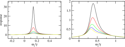
Figure 6: Response spectrum of the polariton gas to an extra laser beam at $\Delta k=0.1\,\mu\rm m$ (left panel) and $\Delta k=0.2\,\mu\rm m$ (right panel) for several values of the signal laser intensity $I_{s}$ marked with the symbols in Fig.5.

This is another important difference as compared to the thermodynamical equilibrium case, where the presence of the external field explicitely breaking the symmetry opens a gap in the real part of the dispersion law magnon . In the present non-equilibrium case the gap appears instead in the imaginary part. The dependence of the gap amplitude $\textrm{Im}[\omega_{G}(\Delta k=0)]$ on the signal laser intensity $I_{s}=|F_{s}|^{2}$ is plotted in the right panel of Fig. 5. Again, the behaviour for low values of $I_{s}$ is a square root one. This can be easily explained by the fact that $\omega_{G}(\Delta k=0)$ is an analytic function of $S,P$ and $I$ and these have the square root dependence on $I_{s}$ shown in the left panel of Fig.5.

The presence of the gap in the Bogoliubov spectrum is expected to have dramatic consequences on the response of the system to the probe laser of wave vector $k_{r}$ and frequency $\omega_{r}$. This can be quantitatively studied by means of the same linear response equation (10) once the correction to the stationary-state amplitudes $S$, $P$ and $I$ due to the presence of the signal laser have been duly taken into account. Note how this merely quantitative change in the entries of the ${\mathcal{L}}$ matrix is enough to destroy the weakly-damped Goldstone branch.

Examples of probe response spectra as a function of the probe frequency $\omega_{r}$ are plotted in Fig. 6 for several values of the signal laser power $I_{s}$ and two different values of the probe wave vector $k_{r}$. It is easy to see that the main consequence of the presence of the signal laser field is to broaden the peak and suppress the strongly peaked response to small $\Delta k$ perturbations. This is in exact correspondance with the Bogoliubov spectra plotted in the right panels of Fig.3.

This characteristic dependence of the probe response on the signal beam intensity constitutes a direct and experimentally accessible signature of the existence of a Goldstone mode which gets destroyed when the signal/idler phases are pinned by the signal beam.

VI Signal frequency mismatch

The discussion of the previous section has assumed the signal laser field to be exactly on resonance with the natural parametric oscillation frequency $\omega_{s}$ of the cavity when this is illuminated by the pump laser alone. Here we shall study the case when the parametric emission is forced by the signal beam to take place at a slightly different frequency $\omega_{s}+\delta\omega_{s}$.

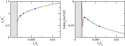
Figure 7: The same as figure 5, but for a signal laser detuning of $\delta\omega_{s}=0.01\,\textrm{meV}$. In the hatched region, the three-mode solution is dynamically unstable (see text).

Two intensity regimes have now to be distinguished for the signal laser. For a small intensity $I_{s}$, the signal beam can be considered as a perturbation of the parametric oscillation state at the natural frequency $\omega_{s}$ and can be introduced within the linear response theory of section IV as a probe beam. Thanks to the detuning $\delta\omega_{s}$, the signal beam is in fact not on resonance with the Goldstone mode, so that its response does no longer diverge as it instead happened in sec.V.

On the other hand, the linearized theory breaks down for larger signal laser intensity, when the parametric oscillation no longer takes place at its natural frequency $\omega_{s}$ but rather appears at the forcing signal beam frequency $\omega_{s}+\delta\omega_{s}$. A stationary state for the mean-field equation (1) of the form:

$$\psi_{LP}(x,t)=P\,e^{i(k_{p}x-\omega_{p}t)}+S\,e^{i(k_{s}x-(\omega_{s}+\delta\omega_{s})t)}+\\ +I\,e^{i(k_{i}x-(\omega_{i}-\delta\omega_{s})t)},$$ (14)

has thus to be considered. The transition from one case to the other can be described by means of a Hopf bifurcation scenario in a theory explicitely including the possibility of a time-dependence for $S$, $P$ and $I$. For the sake of simplicity, we will restrict ourselves in the following to the parameter range well above the bifurcation point, where the ansatz (14) is accurate. The Hopf bifurcation point is signalled by the solution (14) becoming unstable, i.e. the imaginary part of an eigenvalue of the linearized theory becoming positive $\textrm{Im}[\omega(\Delta k=0)]>0$.

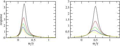
Figure 8: The same as Fig. 6, but for a signal laser detuning of $\delta\omega_{s}=0.01{\textrm{m}eV}$ and for the values of $I_{s}$ indicated with the symbols in Fig.7.

The signal mode occupation $n_{s}$ and the imaginary part $\textrm{Im}[\omega_{G}(\Delta k=0)]$ of the Goldstone mode at $\Delta k=0$ are plotted in respectively the left and right panels of Fig. 7 as a function of the signal beam intensity $I_{s}$. The hatched region is the low $I_{s}$ region where the solution (14) is dynamically unstable. Well above the instability region, the behaviour of $\textrm{Im}[\omega_{G}(\Delta k=0)]$ as a function of the signal laser intensity recovers the behaviour of the zero-detuning $\delta\omega_{s}=0$ case.

Examples of response spectra to the probe beam are shown in Fig.8. For low values of the signal laser intensity $I_{s}$ (but still above the instability threshold) the response is strongly peaked at the weakly damped Goldstone mode, while it broadens for larger values of $I_{s}$: this phenomenology is in close qualitative agreement with the one shown in Fig. 5 for the case of a perfectly tuned signal laser. Provided we are sufficiently far from the Hopf bifurcation, a mismatch in the signal frequency therefore does not substantially affect the signal/idler phase pinning effect which is responsible for the disappearance of the strong response associated to the Goldstone mode.

VII Finite spot

In all the previous discussion, a spatially homogeneous system was considered, with a spatially homogeneous pump beam; in that case, the wave vector was a good quantum number. Real experiments are however performed using finite-size pump laser spots, generally of Gaussian shape $F_{p}(k)\sim\exp[-\sigma_{p}^{2}\,(k-k_{p})^{2}/2]$. This implies that a range of wave vectors are excited, yet the pump, signal and idler beams remain well distinct in $k$ space provided the (real-space) spot size $\sigma_{p}$ is large enough $|k_{p}-k_{s}|\,\sigma_{p}\gg 1$. Under such an hypothesis, the signal and idler phase rotation (6) is still a symmetry element of the problem .

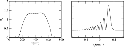
Figure 9: Numerical results for the spatial profile of the signal density (left panel) and the signal wave vector spectrum (right panel) for a pump waist $\sigma_{p}=300\,\mu\rm m$, a carrier pump wave vector $k_{p}=1.57\,\mu\rm m$. The vertical dashed line in the right panel shows the wavevector of the signal emission at the center of the spot. Other parameters as in Fig.2.

The spatial and wave vector distributions of the parametric signal emission are shown in Fig. 9 for the case of a wide pump spot in the absence of any incident signal laser. The plotted curves are the result of a numerical integration of the full mean-field evolution equation (1) until the steady-state is reached: the main feature to note is the inhomogeneous wave vector broadening that can be observed in the right panel, a broadening which always remains much smaller than the wavevector space distance $|k_{p}-k_{s}|\simeq 1.5\,\mu\textrm{m}^{-1}$. A detailed explanation of the physical origin of this broadening is posponed to the forthcoming publication pattern .

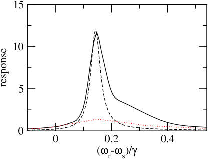
Figure 10: Solid line: response of the polariton pattern of Fig. 9 as a function of frequency, when it is probed by a laser beam with wave vector $k_{r}=0.175\mu\rm m^{-1}$ (full black line). Dashed line: prediction for a homogeneous system with the values at the center of the spot. Red dotted line shows the response when a signal laser with intensity $I_{s}=10^{-3}\,I_{p}$ and waist $\sigma_{s}\gg\sigma_{p}$ is applied to the inhomogeneous system.

The response of this steady-state to an additional probe laser beam with wave vector $k_{r}=0.175$ and a waist $\sigma_{r}=\sigma_{p}$ is shown in Fig. 10. As in the case of an homogeneous system, the very peaked response as a function of frequency is a consequence of the presence of the Goldstone mode. The enhanced broadening as compared to the homogeneous case is mostly due the inhomogeneous broadening of the signal emission in wavevector space shown in fig.9. The top of the peak is in good agreement with the prediction for a homogeneous system with the same signal wave vector as the one actually selected at the center of the finite spot (dashed line). Agreement is observed also in the low-frequency tail of the peak, but differences are apparent in the high-frequency tail: the tail of the finite spot curve extends in fact for much longer than in the homogeneous case. This is a direct consequence of the asymmetric inhomogeneous broadening of the signal wave vectors shown in the right panel of Fig. 9, which indeed mostly extends towards lower $k_{s}$ values. Relative to these wave vectors, the perturbation has a larger $\Delta k=k_{r}-k_{s}$, which means that the response peak lies at higher frequencies and has a larger width (as shown in the lower panels of Fig.3).

The red dotted line in Fig. 10 shows the response when a signal laser beam is applied, which explicitely breaks the $U(1)$ symmetry. Analogously to the case of a homogeneous system, the fact that the $U(1)$ symmetry is now explicitely broken causes a strong broadening of the peak and a corresponding suppression of the peak response. This completes the proof that the concepts and the analytical results developed for the homogeneous case can still be safely applied when the pump spot has a finite size.

VIII Conclusions

In the present paper, we have studied the properties of the Goldstone mode that appears in the elementary excitation spectrum of planar parametric oscillators above threshold as a consequence of the spontaneous breaking of the $U(1)$ signal/idler phase symmetry. Although quantitative predictions have been shown only for the case of planar semiconductor microcavities with a quantum well excitonic transition strongly coupled to the cavity mode, the physics is the same in any kind of parametric oscillator with planar geometry.

Analogies and differences with thermodymical equilibrium systems showing the same spontaneous symmetry breaking phenomenon (e.g. superfluid Helium 4 or Bose-Einstein condensates) have been drawn. In particular, several features have been pointed out, which are typical of the stationary state of a non-equilibrium system where a dynamical equilibrium occurs between driving and losses. Although its dispersion tends as usual to $0$ in the long wavelength limit, the Goldstone mode of our non-equilibrium system is not a propagating mode like zero-sound in Helium or Bose-Einstein condensates, but rather an overdamped mode. A simple way of probing its dispersion at small wavevectors is to measure the response of the system to an additional probe laser shone onto the cavity at an angle close to the signal emission. As the probe beam approaches the signal, the damping rate of the Goldstone mode tends to vanish, which corresponds to a probe response spectrum extremely peaked at the Goldstone mode frequency.

A signal laser beam injected into the cavity and stimulating the parametric emission is shown to provide an external field which explicitely breaks the $U(1)$ symmetry. This in analogy with what happens in a ferromagnet, where an external magnetic field provides a preferential orientation to the magnetization. As usual, the explicit breaking of the symmetry is responsible for the opening of a gap in the Goldstone mode dispersion. Differently from the equilibrium case, the gap is here in the imaginary part of the dispersion. As a consequence, the peak in the response spectrum gets broader and eventually almost disappears when the signal laser intensity grows higher.

In the last sections of the paper, a few issues of experimental relevance in view of the actual observation of the Goldstone mode have been addressed, such as the effect of a slight detuning of the signal laser from the natural parametric oscillation frequency, and the finite size of the excitation spot. All of them are shown not to give any dramatic effect on the observation of the Goldstone mode.

An experimental study along these lines appears therefore feasible with present technology samples and will constitute an important step in the understanding of the properties of parametric oscillation in spatially distributed systems, in particular of its analogies and differences with the Bose-Einstein condensation phase transitions in systems at thermodynamical equilibrium.

Appendix A Equations defining the stationary-state

Substituting the ansatz (5) in the equations of motion (1) and imposing the stationary state leads to the following set of complex equations:

$$0 = \frac{1}{X_{p}^{2}}\left[\epsilon_{p}-i\frac{\gamma}{2}-\omega_{p}\right]\tilde{P}+\left(|\tilde{P}|^{2}+2|\tilde{S}|^{2}+2|\tilde{I}|^{2}\right)\tilde{P}+2\tilde{P}^{\ast}\tilde{S}\tilde{I}+\tilde{F}_{p}$$ (15)

$$0 = \frac{1}{X_{s}^{2}}\left[\epsilon_{s}-i\frac{\gamma}{2}-\omega_{s}\right]\tilde{S}+\left(2|\tilde{P}|^{2}+|\tilde{S}|^{2}+2|\tilde{I}|^{2}\right)\tilde{S}+\tilde{P}^{2}\tilde{I}^{\ast}$$ (16)

$$0 = \frac{1}{X_{i}^{2}}\left[\epsilon_{i}-i\frac{\gamma}{2}-2\omega_{p}+\omega_{s}\right]\tilde{I}+\left(2|\tilde{P}|^{2}+2|\tilde{S}|^{2}+|\tilde{I}|^{2}\right)\tilde{I}+\tilde{P}^{2}\tilde{S}^{\ast}.$$ (17)

The following shorthand notations have been introduced $\epsilon_{p,s,i}=\varepsilon(k_{p,s,i})$ and $X_{p,s,i}=U_{X}(k_{p,s,i})$. Scaled quantities $\tilde{S}=\sqrt{g}\,X_{s}\,S$, $\tilde{P}=\sqrt{g}\,X_{p}\,P$, $\tilde{I}=\sqrt{g}\,X_{i}\,I$ and $\tilde{F}_{p}=\sqrt{g}\,U_{C}(k_{p})/U_{X}(k_{p})\,F_{p}$ have been defined. The complex variables ${\tilde{S}}$, ${\tilde{P}}$, ${\tilde{I}}$, $\omega_{s}$ can be obtained from the set of three complex equations (15-17) together with the condition that the frequency $\omega_{s}$ has to be real: only 7 real equations are then available to determine 8 real variables, which means that the solutions are grouped in 1D manifolds. As the set of equations ((15)-(17)) is symmetric under the phase rotation (6), the solution manifold is generated by the action of (6) on a given solution.

The presence of the signal beam at frequency $\omega_{s}+\delta\omega_{s}$ is taken into account in the set of equations ((15)-(17)) by simply adding the term $\tilde{F}_{s}=\sqrt{g}\,U_{C}(k_{s})/U_{X}(k_{s})\,F_{s}$ to the right-hand side of (16) and considering $\omega_{s}\rightarrow\omega_{s}\pm\delta\omega_{s}$ as a fixed quantity. In this case, the number of unknowns is reduced to three complex variables, which are then completely determined by the three complex equations.

Appendix B Analytical remarks on the Goldstone mode

In this appendix we show that (convective) stability cross implies that only even powers are possible in the expansion of $\textrm{Im}[\omega(k)]$ around $k=0$. The eigenvalues of a linear operator $\mathcal{L}(k)$ have a Taylor expansion around every value of $k$, except for some special points where fractional powers $1/p$ can occur (see Ref.kato , p. 65). If the Taylor expansion exists, stability requires $\textrm{Im}[\omega(k)]<0$ for all $k$, which implies that only even powers of $k$ are allowed in the Taylor expansion of $\textrm{Im}[\omega(k)]$ around $k=0$.

If accidentally $k=0$ is a special point of order $p$, there are $p$ eigenvalues which have a Puiseux series instead of a Taylor series

$$\lambda_{h}(k)=\lambda+\alpha_{1}e^{2\pi ih/p}k^{1/p}+\alpha_{2}e^{4\pi ih/p}k^{2/p}+\cdots,$$ (18)

for $h=0,1,\ldots,p-1$. If $p=2$, stability requires that $\text{Im}(\alpha_{m})=0$ for any odd $m$, so that no half-integer powers are allowed in the expansion of $\textrm{Im}[\lambda(\omega)]$. The case with $p>2$ is ruled out just because it would forcedly give an eigenvalue with positive imaginary part.

In summary, only even powers are allowed in the expansion of $\textrm{Im}[\omega(k)]$, so that the expansion of $\textrm{Im}[\omega(k)]$ is to leading order quadratic (unless this term accidentally vanishes).

Appendix C Comparisons with $\chi^{(2)}$ OPO’s

In this Appendix we make the link of our theory to the different case of an optical parametric oscillator based on a nonlinear medium showing a second-order optical nonlinearity instead of a third order one planar_OPO_2 .

In the non-degenerate case where pump, signal and idler belong to different photonic branches of the planar cavity, the terms of the Hamiltonian responsible for the parametric downconversion process have the form:

$$H_{\rm int}=\hbar g\,\left[{\hat{E}}^{\dagger}_{p}(k_{p})\,{\hat{E}}_{i}(k_{i})\,{\hat{E}}_{s}(k_{s})+{\textrm{h}.c.}\right],$$ (19)

where a single pump photon is converted into a pair of signal/idler photons. An ansatz analogous to (5) can then be used for the stationary state of the three pump, signal and idler fields at mean-field regime:

$$E_{p}(x) \rightarrow P\,e^{i(k_{p}x-\omega_{p}t)}$$ (20)

$$E_{s}(x) \rightarrow S\,e^{i(k_{s}x-\omega_{s}t)}$$ (21)

$$E_{i}(x) \rightarrow I\,e^{i(k_{i}x-\omega_{i}t)},$$ (22)

and the amplitudes $P$, $S$, and $I$, as well as the frequency $\omega_{s}$ are obtained by inserting this ansatz into the field equations of motion for the Hamiltonian (19).

It is appearent that the transformation (6) is still a symmetry of the Hamiltonian (19), which is spontaneously broken above threshold by the ansatz (20-22). A Goldstone mode is therefore present, with the same properties as discussed in the body of the present paper.

The only different lies in the dependence of the stationary state on the pump intensity lugiato_degen_OPO : as the second-order nonlinearity does not produce any direct shift of the mode frequency due to the mode population, the curves of Fig.2 are dramatically modified. In particular, there is no upper threshold for the parametric process, which at high intensities is replaced by chaotic behaviour lugiato_degen_OPO .

In the degenerate case where signal and idler belong to the same photonic $L$ branch, the parametric terms of the parametric Hamiltonian read instead:

$$H_{\rm int}=\hbar g\,\left[{\hat{E}}^{\dagger}_{p}(k_{p})\,{\hat{E}}_{L}(k_{i})\,{\hat{E}}_{L}(k_{s})+{\textrm{h}.c.}\right]$$ (23)

so that the ansatz

$$\psi_{p}(x) \rightarrow P\,e^{i(k_{p}x-\omega_{p}t)}$$ (24)

$$\psi_{L}(x) \rightarrow S\,e^{i(k_{s}x-\omega_{s}t)}+I\,e^{i(k_{i}x-\omega_{i}t)}$$ (25)

has to be used to describe the parametric oscillation state. Also in this case, the equations of motion are invariant with respect to the transformation (6) and all the physics of the Goldstone mode remains unchanged. Note how the transformation (6) corresponds in this case to a spatial translation of the field (25) in the $L$ mode.

The only exception occurs when the system oscillates in a completely degenerate regime $k_{s}=k_{i}=k_{p}/2$ where the signal and the idler coincide: in this case, the $U(1)$ symmetry is reduced to a discrete $\pm$ symmetry and no Goldstone mode is any longer present. A linear analysis for this completely degenerate case has been worked out in lugiato_degen_OPO , where it was shown explicitely that no zero eigenvalue is present for $\Delta k=0$.

Note that the condition characterizing a complete degeneracy regime is weakened for a finite spot of size $\sigma_{p}$, where the pump, signal and idler spots have a $k$-space broadening of the order of $1/\sigma_{p}$. In this case, in fact, the Goldstone mode can be shown to disappear as soon as $\sigma_{p}|k_{s}-k_{i}|\simeq 1$.

References

- (1) K. Huang, Statistical Mechanics (New York, John Wiley & Sons, 1963).
- (2) P.W. Anderson, Phys. Rev. 112, 1900 (1958).
- (3) D. Forster, Hydrodynamic fluctuations, Broken symmetries and correlation functions (W.A. Benjamin, Massachusetts, 1975).
- (4) D. Pines and P. Nozières, The Theory of Quantum Liquids, (Addison-Wesley, Redwood City, CA, 1990), Vol. 2.
- (5) L. D. Landau, E. M. Lifshitz and L. P. Pitaevskii, Statistical Physics, Vol.2, Pergamon Press, Oxford, 1980.
- (6) M. C. Cross and P. C. Hohenberg, Rev. Mod. Phys. 65, 851 (1993).
- (7) see e.g. S. Chandrasekhar, Hydrodynamic and hydromagnetic stability (Clarendon Press, Oxford, 1961).
- (8) M. Vaupel, A. Maître and C. Fabre, Phys. Rev. Lett. 83, 5278 (1999); S. Ducci, N. Treps, A. Maître and C. Fabre, Phys. Rev. A 64, 023803 (2001).
- (9) G.-L. Oppo, M. Brambilla and L.A. Lugiato, Phys. Rev. A 49, 2028 (1994); G.-L. Oppo et al., J. Mod. Opt. 41, 1151 (1994); S. Longhi, Phys. Rev. A 53, 4488 (1996); K. Staliunas, J. Mod. Opt. 42, 1261 (1995).
- (10) N. Gisin et al., Rev. Mod. Phys. 74, 145 (2002).
- (11) J. Baumberg and L. Viña (Eds.) Special issue on Microcavities, [Semicond. Sci. Technol. 18, S279 (2003)].
- (12) B. Deveaud (Ed.), Special issue on the “Physics of semiconductors microcavities”, Phys. Stat. Sol. B 242, 2145-2356 (2005) and references therein.
- (13) P. G. Savvidis, J. J. Baumberg, R. M. Stevenson, M. S. Skolnick, D. M. Whittaker and J. S. Roberts, Phys. Rev. Lett. 84, 1547 (2000).
- (14) R. M. Stevenson, V. N. Astratov, M. S. Skolnick, D. M. Whittaker, M. Emam-Ismail, A. I. Tartakovskii, P. G. Savvidis, J. J. Baumberg and J. S. Roberts, Phys. Rev. Lett 85, 3680 (2000).
- (15) R. Houdré, C. Weisbuch, R. P. Stanley, U. Oesterle and M. Ilegems, Phys. Rev. Lett. 85, 2793 (2000).
- (16) A. Baas, J.-Ph. Karr, M. Romanelli, A. Bramati and E. Giacobino Phys. Rev. Lett. 96, 176401 (2006).
- (17) L.P. Pitaevskii and S. Stringari, Bose-Einstein Condensation, Clarendon Press Oxford (2003).
- (18) I. Carusotto and C. Ciuti, Phys. Rev. Lett. 93, 166401 (2004); C. Ciuti and I. Carusotto, Phys. Stat. Sol. (b) 242, 2224 (2005).
- (19) R. Zambrini et al., Phys. Rev. A 62, 063801 (2000).
- (20) M. Wouters and I. Carusotto, cond-mat/0512464.
- (21) P.G. Savvidis, C. Ciuti, J. J. Baumberg, D. M. Whittaker, M. S. Skolnick, J. S. Roberts, Phys. Rev. B 64, 075311 (2001); J.J. Baumberg and P.G. Lagoudakis, Phys. Stat. Sol. (b) 242, 2210 (2005).
- (22) V. Savona, P. Schwendimann and A. Quattropani, Phys. Rev. B 71, 125315 (2005).
- (23) D.M. Whittaker, Phys. Rev. B 71, 115301 (2005).
- (24) C. Ciuti, P. Schwendimann and A. Quattropani, Semicond. Sci. Technol. 18, S279-S293 (2003).
- (25) G.P. Agrawal and R.W. Boyd, Contemporary Nonlinear Optics (Academic Press, 1992).
- (26) D. F. Walls and G. J. Milburn, Quantum Optics (Springer, Berlin, 1994).
- (27) P. N. Butcher and D. Cotter The Elements of Nonlinear Optics, (Cambridge University Press, 1990)
- (28) M. Wouters and I. Carusotto in preparation.
- (29) A. I. Tartakovskii, D.N. Krizhanovskii, D. A. Kurysh, V. D. Kulakovskii, M. S. Skolnick, and J. S. Roberts, Phys. Rev. B 65, 081308(R) (2002).
- (30) J.Y. Courtois et al., J. Mod. Opt. 38, 177 (1991).
- (31) L. P. Pitaevskii and S. Stringari, Phys. Lett. A 235, 398 (1997).
- (32) V. DeGiorgio and M.O. Scully, Phys. Rev. A 2, 1170 (1970).
- (33) M. O. Scully, M. S. Zubairy, Quantum Optics, Cambridge University Press (1997).
- (34) R. Neubecker and A. Zimmermann, Phys. Rev. E 65, 035205(R) (2002); R. Neubecker and O. Jakoby, Phys. Rev. E 67, 066221 (2003).
- (35) L. Sneddon, Phys. Rev. A 24, 1629 (1981).
- (36) T. Kato Perturbation theory for linear operators, second edition, Springer-Verlag Berlin (1984).
- (37) L. A. Lugiato et al., Il Nuovo Cimento 10, 959 (1988).