A mean-field theory for strongly disordered non-frustrated antiferromagnets

Abstract

Motivated by impurity-induced magnetic ordering phenomena in spin-gap materials like TlCuCl₃, we develop a mean-field theory for strongly disordered antiferromagnets, designed to capture the broad distribution of coupling constants in the effective model for the impurity degrees of freedom. Based on our results, we argue that in the presence of random magnetic couplings the conventional first-order spin-flop transition of an anisotropic antiferromagnet is split into two transitions at low temperatures, associated with separate order parameters along and perpendicular to the field axis. We demonstrate the existence of either a bicritcal point or a critical endpoint in the temperature–field phase diagram, with the consequence that signatures of the spin flop are more pronounced at elevated temperature.

I Introduction

The interplay of magnetism and disorder is a fascinating field of research in condensed matter physics. Various non-trivial low-temperature phases, like spin glasses, Bose glasses, random singlet phases etc., and associated phase transitions have been studied in both theory and experiment. A particularly interesting manifestation of quantum effects is impurity-induced magnetism in quantum paramagnets: The starting point is a Mott insulator with a finite spin gap which separates elementary spin excitations from the spin singlet ground state; examples are SrCu₂O₃, CuGeO₃, PbNi₂V₂O₈, SrCu₂(BO₃)₂, KCuCl₃, or TlCuCl₃. As demonstrated in recent experiments,exp1 ; exp2 ; exp3 ; exp3b ; exp4 ; exp5 ; sitetlcucl ; dopeins non-magnetic impurities, replacing magnetic ions in such quantum paramagnets, can induce effective magnetic moments. These impurity-induced moments reveal themselves in a Curie-like behavior of the uniform susceptibility, $\chi\propto C/T$, at intermediate temperatures. Remarkably, in the presence of three-dimensional couplings these induced moments can order at sufficiently low temperatures, thus changing the spin-gapped paramagnetic ground state of the pure compound into an magnetically long-range ordered state upon doping.

On the theoretical side, the appearance of effective moments upon doping vacancies into the spin system is well understood in principle. It occurs in systems with confined spinons, i.e., elementary $S=1$ excitations; for spin $1/2$ systems it is best visualized in terms of broken singlet bonds where one spin is replaced by a vacancy. The liberated spin $1/2$ is confined to the vacancy at low energies, resulting in an effective spin $1/2$ moment.sigrist ; icmp (In contrast, in host systems with elementary $S=1/2$ excitations, i.e., deconfined spinons, no moments are generated by introducing vacancies.) This theoretical picture has been supported by various numerical studies, in particular on spin chainbruce and ladder systems.elbio ; Miyazaki ; Yasuda

A number of theoretical works also addressed impurity-induced antiferromagnetic ordering. On the one hand, numerical simulations on finite-size systems of spin gap magnets containing impurities studied signatures of magnetic ordering.Yasuda ; wessel ; rosc1 ; rosc2 On the other hand, analytical approachesfabrizio ; melin ; rsrg1 ; rsrg2 typically start from an effective spin-$1/2$ model involving the impurity-induced moments $\vec{S}_{i}$ only:

$$\mathcal{H}_{\rm eff}=\sum_{ij}J_{ij}\vec{S}_{i}\cdot\vec{S}_{j},$$ (1)

where the interaction $J_{ij}$ between two impurity moments depends on their distance $r_{ij}$ as $J_{ij}\propto\exp(-r_{ij}/\xi)$, where $\xi$ is the magnetic correlation length of the host material. Due to the random locations of the impurities the system shows a broad distribution of coupling values $J_{ij}$. Furthermore, on bipartite lattices the sign of $J_{ij}$ will alternate as function of the Manhattan distance between $i$ and $j$. This implies that classically all bonds can be satisfied with a Neél-type arrangement of the effective moments. In other words, Eq. (1) defines a strongly disordered non-frustrated quantum magnet. Real-space renormalization group studiesrsrg1 ; rsrg2 indicate that the ground state of the model (1) with quantum spins 1/2 shows long-range order for any concentration of impurity moments; this is supported by numerical simulations of vacancy-doped quantum paramagnets with confined spinons, which display magnetic order up to the percolation threshold.Yasuda ; wessel ; rosc1 ; rosc2 Thus, although the systems under consideration are long-range-ordered antiferromagnets, their properties can be expected to be strongly different from that of antiferromagnets without quenched disorder, due to the broadly distributed $J_{ij}$.

The purpose of this paper is to introduce a generalized mean-field theory, which takes into account the broad distribution of coupling constants in Eq. (1). The central idea is to parameterize the spins according to their coupling strength to the environment, i.e., by their sum of coupling constants to all other spins, $\bar{J}$, see Eq. (2) below. For each $\bar{J}$ a separate mean-field parameter will be introduced, leading to integral equations replacing the standard self-consistency relations. Although such a mean-field theory misses certain aspects of disorder physics, like localization phenomena, we will demonstrate that it captures various distinct properties of magnets described by Eq. (1). For instance, the overall behavior of the order parameter as function of temperature is significantly different from non-disordered magnets and from conventional mean-field theory. In particular, we discuss the physics in an external field the presence of a magnetic anisotropy, relevant for most real materials. Here, a spin-flop transition is expected to occur for fields parallel to the easy axis, which indeed has been observed in TlCu_1-xMg_xCl₃.sitetlcucl We argue that strong disorder leads to an interesting temperature evolution of the spin-flop physics: at low temperature the transition is generically split into two (with at least one of them being continuous), whereas at elevated temperature a single first-order transition is restored.

The bulk of the paper is organized as follows: In Sec. II we describe our generalized mean-field theory, together with the numerical procedure to solve the mean-field equations. Sec. III discusses the symmetries and possible phases of the model in the presence of a field parallel to the easy axis, and presents temperature–field phase diagrams obtained from the mean-field theory. In Sec. IV we take a closer look at the phase transitions, in particular at the spin-flop transition. A comparison to experiments and available numerical results for vacancy-doped magnets is given in Sec. V. A brief outlook concludes the paper.

II Mean-field theory

II.1 Parameterization

In standard mean-field theory, the many-body problem is reduced to one single-spin problem in an effective field. Following this idea in the presence of disorder requires to consider distinct effective fields for all spins. Physicswise, we expect spins to behave differently if they have different couplings to their environment; spins in a similar environment may behave in a similar fashion. This is the basis for the main simplification of our mean-field theory: We will parameterize the spins by the coupling sum $\bar{J}$, defined as

$$\bar{J}_{i}=\sum_{j}J_{ij}(-1)^{i-j+1}=\sum_{j}|J_{ij}|.$$ (2)

Thus we replace the spin variables $\vec{S}_{i}$ by $\vec{S}(\bar{J})$. The factor $(-1)^{i-j+1}$ accounts for the sublattice structure of the bipartite lattice, with $(i-j)$ being the Manhattan distance, and the second identity follows from the alternating sign of the coupling $J_{ij}$. With this definition, $\bar{J}_{i}$ is the magnitude of the effective field on spin $i$ in a perfectly ordered antiferromagnetic state.

For a description of the magnetic interactions in terms of the coupling sum, we introduce a probability distribution $P(\bar{J})$ according to

$$P(\bar{J})=\frac{1}{N}\sum_{i}\delta({\bar{J}}-\bar{J}_{i})$$ (3)

where $N$ is the number of spins. Further, we need an interaction function $f(\bar{J}_{1},\bar{J}_{2})$, defined as

$$f(\bar{J}_{1},\bar{J}_{2})=\frac{1}{NP(\bar{J}_{1})P(\bar{J}_{2})}\sum_{ij}|J_{ij}|\delta({\bar{J}_{1}}-\bar{J}_{i})\delta({\bar{J}_{2}}-\bar{J}_{j})\,.$$ (4)

which is symmetric w.r.t. to $\bar{J}_{1}\leftrightarrow\bar{J}_{2}$ and fulfills normalization conditions

$$\int d\bar{J}_{2}P(\bar{J}_{2})f(\bar{J}_{1},\bar{J}_{2})=\bar{J}_{1}\,.$$ (5)

With these definitions, a ferromagnetic Heisenberg model, $\mathcal{H}=-\sum_{ij}J_{ij}\vec{S}_{i}\cdot\vec{S}_{j}$, takes the form

$$\mathcal{H}=-N\int d\bar{J}_{1}d\bar{J}_{2}P(\bar{J}_{1})P(\bar{J}_{2})f(\bar{J}_{1},\bar{J}_{2})\vec{S}(\bar{J}_{1})\cdot\vec{S}(\bar{J}_{2}).$$ (6)

Defining an effective field

$$\vec{m}(\bar{J})=\int d\bar{J}_{2}P(\bar{J}_{2})f(\bar{J},\bar{J}_{2})\langle\vec{S}(\bar{J}_{2})\rangle,$$ (7)

the mean-field Hamiltonian reads

$$\mathcal{H}_{\rm mf}=-N\int d\bar{J}P(\bar{J})\left[\vec{m}(\bar{J})+\vec{B}\right]\cdot\vec{S}(\bar{J}),$$ (8)

where we have included an external field $\vec{B}$.

For an antiferromagnet on a bipartite lattice different mean fields are required for the two sublattices A and B, which can become inequivalent in the presence of symmetry breaking and a finite field. Using $P_{A}(\bar{J})=P_{B}(\bar{J})=P(\bar{J})/2$, the effective field becomes

$$\vec{m}_{A,B}(\bar{J})=\pm\int d\bar{J}_{2}P(\bar{J}_{2})f(\bar{J},\bar{J}_{2})\frac{\langle\vec{S}_{A}(\bar{J}_{2})\rangle-\langle\vec{S}_{B}(\bar{J}_{2})\rangle}{2}.$$ (9)

The corresponding mean-field Hamiltonian reads

$$\begin{split}\mathcal{H}_{\rm mf}=-\frac{N}{2}\int d\bar{J}P(\bar{J}&)\left(\left[\vec{m}_{A}(\bar{J})+\vec{B}\right]\vec{S}_{A}(\bar{J})+\right.\\ &\left.+\left[\vec{m}_{B}(\bar{J})+\vec{B}\right]\vec{S}_{B}(\bar{J})\right)\end{split}$$ (10)

replacing (8).

In general, two angles are needed to specify the orientation of a spin. In the following, we will exclusively consider situations where $\mathcal{H}$ has a U(1) symmetry of rotations about the $z$ axis (see Sec. III). Then we can describe the orientation of a spin just by one angle, $\varphi$, between spin and $z$ axis; the angle in the $xy$ plane can be fixed to zero, positive (negative) values of $\varphi$ on the A (B) sublattice account for the staggered in-plane order. Hence, the expectation value of a spin can be written in the following way:

$$\langle\vec{S}_{A,B}(\bar{J})\rangle=\left|\langle\vec{S}_{A,B}(\bar{J})\rangle\right|\left(\begin{array}[]{c}\sin\varphi_{A,B}(\bar{J})\\ 0\\ \cos\varphi_{A,B}(\bar{J})\\ \end{array}\right).$$ (11)

The single-spin problem of Eq. (8) can be readily solved, yielding the mean-field equations:

$$\cos\varphi_{A,B}(\bar{J})=\vec{e_{z}}\cdot\frac{[\vec{B}+\vec{m}_{A,B}(\bar{J})]}{|\vec{B}+\vec{m}_{A,B}(\bar{J})|}\,,$$ (12a)

and

$$\left|\langle\vec{S}_{A,B}(\bar{J})\rangle\right|=s\tanh\frac{\left|\vec{B}+\vec{m}_{A,B}(\bar{J})\right|}{k_{B}T/s}\,.$$ (12b)

The amplitude equation (12b) has been written for a spin with two states $\pm s$, appropriate for quantum spins $s=1/2$ – this will be used in the numerical calculations. For continuous classical spins the $\tanh()$ needs to be replaced by a Brillouin function as usual.

In the case of $P(\bar{J})=\delta(\bar{J}-\bar{J}_{0})$ and $f(\bar{J}_{1},\bar{J}_{2})=\bar{J}_{0}$ the mean-field equations (9,12) reduce to the self-consistency equation of the familiar Weiss mean-field theory, with $\bar{J}_{0}=zJ$ for a Hamiltonian with a nearest-neighbor coupling strength $J$ and a coordination number of $z$.

II.2 Magnetic anisotropy

In this paper we consider the formally simplest source of magnetic anisotropy, namely an anisotropic exchange interaction of easy-axis type (the behavior in the presence of a Dshyaloshinski-Moriya interaction is expected to be similar). Thus, in the Hamiltonian we perform the replacement

$$J_{ij}\vec{S}_{i}\cdot\vec{S}_{j}~{}\rightarrow~{}J_{ij}\left[\beta(S_{i}^{x}S_{j}^{x}+S_{i}^{y}S_{j}^{y})+S_{i}^{z}S_{j}^{z}\right]$$ (13)

with an anisotropy constant $\beta<1$; we keep the coupling to the external field as $\vec{B}\cdot\vec{S}$. We note that in the context of impurity-induced magnetism, e.g., in TlCuCl₃ some complications arise (which we will ignore here): The anisotropy of the effective interaction will depend on the external field and the interaction itself; furthermore the form of the field coupling will be modified, leading to an anisotropic $g$ tensor.

The anisotropy according to Eq. (13) requires the following replacement in the mean-field equations (12):

$$\vec{m}_{A,B}~{}\rightarrow~{}\left(\begin{array}[]{c}\beta m^{x}_{A,B}\\ \beta m^{y}_{A,B}\\ m^{z}_{A,B}\\ \end{array}\right)$$ (14)

where $m^{xy}$ and $m^{z}$ denote the components perpendicular and parallel to the easy axis.

II.3 Choice of input parameters

The described mean-field theory requires the coupling distribution $P(\bar{J})$, Eq. (3), and the interaction function $f(\bar{J}_{1},\bar{J}_{2})$, Eq. (4), as input. Both functions are given by the underlying microscopic model. We have numerically determined $P(\bar{J})$ and $f(\bar{J}_{1},\bar{J}_{2})$ for an effective model of impurity-induced order in quantum paramagnets, Eq. (1), as described in the Appendix.

For the actual mean-field calculations we found it more convenient to use plausible model (i.e. fitting) functions instead. However, a difficulty arises here: $P(\bar{J})$ and $f(\bar{J}_{1},\bar{J}_{2})$ cannot be chosen independently, because the normalization conditions (5) cannot be easily fulfilled while preserving the symmetry w.r.t. $\bar{J}_{1}\leftrightarrow\bar{J}_{2}$. We have therefore resorted to the following construction. From an arbitrary symmetric “generating” function $g(\bar{J}_{1},\bar{J}_{2})$ we define the functions $P(\bar{J})$ and $f(\bar{J}_{1},\bar{J}_{2})$ according to:

$$P(\bar{J})=\frac{a}{\bar{J}}\int d\bar{J}_{2}g(\bar{J},\bar{J}_{2})$$ (15)

and

$$f(\bar{J}_{1},\bar{J}_{2})=a\frac{g(\bar{J}_{1},\bar{J}_{2})}{P(\bar{J}_{1})P(\bar{J}_{2})}\,.$$ (16)

Choosing the normalization factor as

$$a^{-1}=\int d\bar{J}_{1}\frac{1}{\bar{J}_{1}}\int d\bar{J}_{2}g(\bar{J}_{1},\bar{J}_{2}),$$ (17)

all normalization conditions are fulfilled.

Figure 1: Model functions for the coupling-sum distribution $P(\bar{J})$ obtained from different generating functions $g(\bar{J}_{1},\bar{J}_{2})$: a) Lognormal-like distribution from Eq. (18), with the parameters $\sigma_{2}=0.699$, $\mu_{L}=-0.171$, $\sigma_{L}=1.3$, and $\bar{J}_{\text{max}}=4.317$. b) Gauss-like distribution from Eq. (19), with the parameters $\mu_{1}=0.59$, $\sigma_{1}=0.289$, $\sigma_{2}=0.193$, and $\bar{J}_{\text{max}}=1.929$. In both cases, $\int d\bar{J}P(\bar{J})=1$.

As detailed in the Appendix, in vacancy-doped magnets the function $P(\bar{J})$ will be peaked at a value which increases with impurity concentration, and it will be increasingly asymmetric at low concentrations, with a tail to higher $\bar{J}$. Thus, among others, we have employed the following generating functions $g(\bar{J}_{1},\bar{J}_{2})$.

$$\begin{split}g(\bar{J}_{1},\bar{J}_{2})&=\exp\left(-\frac{(\ln(\bar{J}_{1})-\mu_{L})^{2}}{2\sigma_{L}^{2}}\right)\exp\left(-\frac{(\ln(\bar{J}_{2})-\mu_{L})^{2}}{2\sigma_{L}^{2}}\right)\\ &\times\exp\left(-\frac{(\bar{J}_{1}-\bar{J}_{2})^{2}}{2\sigma_{2}^{2}}\right)\theta(\bar{J}_{\text{max}}-\bar{J}_{1})\theta(\bar{J}_{\text{max}}-\bar{J}_{2})\end{split}$$ (18)

generates a Lognormal-like distribution $P(\bar{J})$ which captures the coupling distribution for a small impurity concentration. In contrast,

$$\begin{split}g(\bar{J}_{1},\bar{J}_{2})&=\bar{J}_{1}\bar{J}_{2}\exp\left(-\frac{(\bar{J}_{1}-\mu_{1})^{2}}{2\sigma_{1}^{2}}\right)\exp\left(-\frac{(\bar{J}_{2}-\mu_{1})^{2}}{2\sigma_{1}^{2}}\right)\\ &\times\exp\left(-\frac{(\bar{J}_{1}-\bar{J}_{2})^{2}}{2\sigma_{2}^{2}}\right)\theta(\bar{J}_{\text{max}}-\bar{J}_{1})\theta(\bar{J}_{\text{max}}-\bar{J}_{2})\end{split}$$ (19)

leads to a Gauss-like distribution $P(\bar{J})$, corresponding to higher impurity concentrations. The $\mu_{i}$ and $\sigma_{i}$ are free parameters. Examples for the resulting $P(\bar{J})$ are shown in Fig. 1; here and in the following the $\bar{J}$ values are scaled such that the mean value of $\bar{J}$ is unity. In Fig. 8 below we show $P(\bar{J})$ results of the numerical simulations for comparison.

To model an easy-axis situation, we have chosen the anisotropy parameter $\beta=0.9$.

III Phase diagrams

III.1 Symmetries and phases

We will restrict our attention to magnetic fields parallel to the easy axis in which case interesting spin-flop physics arises. Then, the symmetry of the antiferromagnetic Hamiltonian (10) in the presence of a field is U(1) $\times$ Z₂ (whereas for $B=0$ we have U(1) $\times$ Z₂ $\times$ Z₂ which becomes SU(2) $\times$ Z₂ in the absence of exchange anisotropy). Here we have assumed a unit cell size of 2 sites, and the Z₂ symmetry corresponds to the exchange of the two sublattices.

The possible phases are easily enumerated: (i) An Ising phase, where spins on the A (B) sublattice point preferrentially up (down). This breaks the Z₂ symmetry, but leaves the U(1) rotations about the $z$ axis intact. (ii) A canted phase, where the spins order spontaneously perpendicular to the field, and have a finite component in the field direction (equal for both sublattices) as well. Z₂ and U(1) are broken, but a combination of sublattice exchange and 180^o rotation is an intact Z₂ symmetry. (iii) A mixed phase where Z₂ and U(1) are fully broken. (iv) A disordered phase with no symmetry breaking. For non-zero field the spins point in the field direction only.

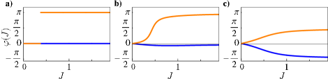
Figure 2: (color online) Angle configurations $\varphi(\bar{J})$ occurring in the ordered phases of the antiferromagnet with field parallel to the easy axis, with blue/red (dark/gray) showing $\varphi_{A}$/$\varphi_{B}$. a) Ising phase, b) mixed phase, c) canted phase. The evolution from a) to c) represents the behavior at low temperatures upon increasing the field, see Figs. 3,4 below.

The order parameters are the components of the staggered magnetization parallel and perpendicular to the direction of the applied magnetic field, $M_{\text{stagg},z}$ and $M_{\text{stagg},xy}$. Further, the ordered phases (i)–(iii) can be nicely characterized by the angles $\varphi$, Eq. (11). Without quenched disorder, i.e., for $P(\bar{J})=\delta(\bar{J}-\bar{J}_{0})$, we have (i) Ising: $\varphi_{A}=0$, $\varphi_{B}=\pi$; (ii) canted: $0<\varphi_{B}=-\varphi_{A}<\pi$; (iii) mixed: $\varphi_{A}<0$, $\varphi_{B}>0$, $|\varphi_{A}|\neq|\varphi_{B}|$. In the disordered case with broad $P(\bar{J})$, the angles become functions of $\bar{J}$, with examples for $\varphi_{A,B}(\bar{J})$ shown in Fig. 2.

III.2 Numerical iteration of the mean-field equations

For given functions $P(\bar{J})$ and $f(\bar{J}_{1},\bar{J}_{2})$ and fixed values of applied magnetic field $\vec{B}$, temperature $T$, and anisotropy constant $\beta$ one can iterate the mean-field equations (9,12), using a linear discretization for the $\bar{J}$ values. The initial distributions for the angles $\varphi_{A,B}(\bar{J})$ and amplitudes $|\langle\vec{S}_{A,B}\rangle|$ could be chosen random in principle; we found it more convenient to employ distributions corresponding to perfect Ising or XY order instead. The mean fields are calculated from Eq. (9); new amplitudes are obtained from Eq. (12b). Some care is required with the angle equation (12a) in the case of an Ising initial configuration: in addition to Eq. (12a) we used an update scheme where spins on the sublattice B flipping from $\varphi_{B}=\pi$ to $\varphi_{B}=0$ are set to $\varphi_{B}=\pi/2$ by hand in order to mix the symmetry breakings.

These different initial conditions and different update schemes lead to potentially different fixed-point distributions after convergence is reached. These correspond to different local minima in the free-energy landscape; comparison of the free energies then yields the stable phase.

III.3 Phase diagrams from mean-field theory

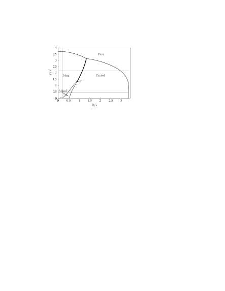
Figure 3: Temperature–field phase diagram of a disordered easy-axis antiferromagnet, obtained from the present mean-field theory, for the Lognormal-like distribution of coupling constants $P(\bar{J})$ as shown in Fig. 1a. The calculation was done for spins with eigenvalues $\pm s$, hence the axes are scaled by appropriate powers of $s$. First-order transitions (thick lines) were determined from crossing points of the free energy, whereas second-order transitions were obtained from extrapolations of the order parameters. BP is a bi-critical point. Magnetization data along the dotted gray lines will be shown in Figs. 5, 7 below.

In Figs. 3, 4 we show representative phase diagrams for the disordered easy-axis antiferromagnet with a longitudinal field, obtained from solving the mean-field equations (9,12). At zero field, the Ising order, present at low temperatures $T$, is destroyed at a continuous transition to a paramagnetic phase. Applying a field to the Ising phase drives various transitions, resulting in a canted phase at intermediate fields and finally a field-polarized (disordered) phase at large field. The main difference to the text-book antiferromagnet is the presence of a mixed phase. The conventional first-order spin-flop transition is split into two transitions at low $T$: At some small field, there is a continuous transition from the Ising to a mixed phase, where an in-plane staggered magnetization $M_{stagg,xy}$ perpendicular to the field develops. Only at a larger field, the Ising order measured by $M_{stagg,z}$ is destroyed, leading to a spin-flop transition into a canted phase, see Figs. 5, 6. The origin of this behavior lies in the broadly distributed couplings: Already for small fields, weakly coupled spins with $\bar{J}\ll B$ cannot sustain the zero-field Ising order and flip in the field direction, while for strongly coupled spins ($\bar{J}\gg B$) Ising order is favored. At low $T$, spins with $\bar{J}\approx B$ reach their lowest-energy state by canting – this results in an overall mixed phase and can be nicely seen in Fig. 2b. (However, at elevated temperatures the in-plane mean-field from these spins alone is not sufficient to establish a mixed phase.) At the spin-flop transition (mixed$\rightarrow$canted at low $T$, Ising$\rightarrow$canted at higher $T$), the spins with the largest couplings loose their Ising order. The evolution of the angle distributions $\varphi_{A,B}(\bar{J})$ with increasing field at low $T$ is shown in Fig. 2.

Note that the part of the phase transition line between Ising and mixed phases at small $T$ and $B$ (dashed) is difficult to extract numerically for a linear discretization of $\bar{J}$. However, by a comparison of energies it is easy to prove that at $T=0$, $B>0$ the Ising phase is always unstable towards the mixed phase for distributions $P(\bar{J})$ which are non-zero for arbitrarily small $\bar{J}$.

Figure 4: Temperature–field phase diagram as in Fig. 3, but for the Gauss-like distribution $P(\bar{J})$ shown in Fig. 1b. (CE is a critical endpoint.)

The two phase diagrams in Figs. 3, 4 differ in the extensions of the mixed phase, and in the character of the phase transition line between mixed and canted phase (see below). Clearly, the deviations from the textbook spin-flop behavior of non-disordered antiferromagnets are most pronounced for broad distributions $P(\bar{J})$.

Both the Néel temperature $T_{N}$ and the critical field $B_{c}$ where long-range order is destroyed, scale with the mean value of the exchange constant (which is set to unity in our calculations). Similarly, the flop field $B_{\rm flop}$ scales as $(1-\beta)^{1/2}$ times the mean exchange. Furthermore, an asymmetric distribution $P(\bar{J})$ as the one in Fig. 1a leads to a larger $T_{N}$, $B_{c}$, $B_{\rm flop}$ compared to a symmetric one with the same mean $\bar{J}$, the reason being that the scales are primarily determined by the spins with large $\bar{J}$.

IV Phase transitions and critical properties

IV.1 Magnetizations and critical exponents

The Figs. 5, 6 show curves for the staggered magnetizations ($M_{\text{stagg},xy}$ and $M_{\text{stagg},z}$) as well as the total magnetization $M$, along the gray dotted lines in the phase diagrams in Figs. 3, 4. The role of $M_{\text{stagg},xy}$ and $M_{\text{stagg},z}$ as order parameters can be clearly seen.

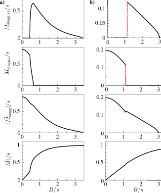
Figure 5: (color online) Magnetization curves for the Lognormal-like distribution $P(\bar{J})$, Fig. 1a, at a) $T/s^{2}=0.435$ and b) $T/s^{2}=2.177$. The red (dashed) part indicates the jump at the first-order transition.

Figure 6: (color online) As Fig. 5, but for the Gauss-like distribution $P(\bar{J})$, Fig. 1b, at a) $T/s^{2}=0$ and b) $T/s^{2}=0.675$.

Fig. 7 shows the total staggered magnetization vs. temperature for both coupling-sum distributions. The transition to the disordered phase at high $T$ (or $B$) is always continuous. The corresponding order-parameter exponent $\beta$, defined through $M_{\text{stagg}}\propto(T_{c}-T)^{\beta}$, should be $1/2$ in conventional mean-field theory. Interestingly, Fig. 7a shows an overall behavior very different from this standard square-root law. This is again due to the broadly distributed couplings: Close to $T_{c}$ the magnetization is effectively only carried by a small fraction of the spins with large $\bar{J}$ – note that the distribution $P(\bar{J})$ corresponding to Fig. 7a has a pronounced tail at larger $\bar{J}$. We note that asymptotically close to the phase transition standard mean-field behavior is restored within the present approach, with exponent $\beta=1/2$.

Figure 7: Staggered magnetization for a) the Lognormal-like distribution $P(\bar{J})$, Fig. 1a, at $B/s=0.209$, and b) the Gauss-like distribution $P(\bar{J})$, Fig. 1b, at $B/s=0.189$.

IV.2 Spin-flop transition

In a non-disordered easy-axis antiferromagnet, a first-order spin-flop transition from an Ising to a canted phase occurs upon increasing the field, leading to a jump in the total magnetization.

In the present situation with quenched disorder, a mixed phase with both $M_{\text{stagg},xy}$ and $M_{\text{stagg},z}$ non-zero occurs at low temperatures. The spin-flop transition splits; for small disorder (a narrow distribution $P(\bar{J})$) the mixed$\rightarrow$canted transition remains of first order, but becomes second-order at larger disorder, whereas the Ising$\rightarrow$mixed transition is always continuous. As the mixed phase only exists at low $T$, the conventional first-order spin-flop transition is restored at elevated temperatures. This has the remarkable consequence that the jump in the magnetization is most pronounced at intermediate $T$, namely at the position of the critical end point or the bicritical point, respectively (see Figs. 5, 6). In general, the magnetization jump is larger in situations with less disorder because the collective spin flop is carried by a larger fraction of spins here.

V Relation to vacancy-doped magnets

In the previous sections, we have described a general mean-field theory for disordered non-frustrated antiferromagnets. We now discuss the applicability to impurity-induced magnetic order in quantum paramagnets.

V.1 Experiments

The low-energy physics of Mg-doped TlCuCl₃ may be expected to be well described by a Hamiltonian of the form (1), provided that the impurity concentration is small. Magnetization measurementssitetlcucl have indicated the presence of a spin-flop transition at 1.8 K for fields parallel to the easy axis [2,0,1] at a field of approximately 0.35 T, significantly below the field corresponding to the bulk gap, 6 T. Interestingly, the spin-flop field seems to be almost independent of the impurity concentration (in the measured range of 0.8 – 2.5%). Our theory does not offer an easy explanation for that: As discussed above, the spin-flop field $B_{\rm flop}$ is roughly proportional to the mean exchange (for fixed anisotropy parameter $\beta$), which would result in a concentration dependence of $B_{\rm flop}$. Within the effective model (1), it is hard to envision a mechanism leading to a concentration-independent flop field, therefore we speculate that correlations between the impurities beyond this effective model play a role here. We also consider it possible that $B_{\rm flop}$ will actually decrease for impurity concentrations smaller than the ones measured. In this context we note that the experiments of Ref. fujisawa, mapped out the phase diagram for TlCuCl₃ doped with 1% Mg and showed the zero-field impurity-induced ordered phase to be continuously connected to the high-field bulk ordered phase. Together with recent theoretical studies mikeska ; rosc1 , this suggests that the impurity and bulk energy scales are not well separated there, i.e., the impurity concentration is too high to allow for a description using the effective model (1).

Further magnetization measurements on Mg-doped TlCuCl₃ would also be interesting regarding the temperature dependence of the spin-flop physics: Our theory predicts interesting behavior for very low temperatures, where the spin-flop transition should split. This requires measurements down to e.g. 1/10th of the ordering temperature $T_{N}$; the experiments of Ref. sitetlcucl, have $T\gtrsim T_{N}/2$.

V.2 Numerical results from Quantum Monte Carlo simulations

Numerical simulations using Quantum Monte Carlo techniques can go beyond the effective model (1) and study the full system, i.e., quantum paramagnet plus vacancies. Those calculations have been reported in Refs. Yasuda, ; wessel, ; rosc1, ; rosc2, , but all were restricted to the spin-isotropic situation. These simulations mapped out the complete phase diagram, with distinct low-field and high-field ordered phases. Among the interesting aspects are the occurrence of Bose glass phases near the bulk field-ordered phase rosc1 , and of a quantum disordered phase at intermediate fields where impurity-induced transverse order is destroyed and the impurity moments appear to form a random-singlet-like phase rosc2 . Clearly, these properties rely on the one hand on the quantum nature of the impurity-induced spin-$1/2$ moments and on the other hand on localization effects, both not captured by our mean-field approach. Quantum Monte Carlo calculations for the spin-anisotropic case studied by us would be interesting, but may be difficult due to the small energy scales involved in the spin-flop physics.

VI Conclusions

We have proposed a mean-field theory for strongly disordered magnets, which takes into account the broad distribution of energy scales in the system. Parameterizing the spins by their sum of coupling constants, equivalent to the exchange field in a perfectly ordered state, yields a continuous set of mean-field equations. We have applied the formalism to a model for impurity-induced order in spin-gap quantum magnets, and derived detailed phase diagrams as function of temperature and external field. We have shown that the conventional first-order spin-flop transition generically splits at low temperatures, leaving room for a mixed phase with both transverse and longitudinal order.

We envision our approach of continuous mean fields to be applicable to a number of interesting problems involving strong disorder, like magnetic ordering in dilute magnetic semiconductors xin , charge ordering in the presence of strong pinning, or electronic models treated within modifications of dynamical mean-field theory (DMFT) sdmft .

Appendix A Coupling constants for impurity-induced moments in paramagnets

Our mean-field theory requires the knowledge of the distribution of the coupling-constant sums, $P(\bar{J})$, and the interaction function $f(\bar{J}_{1},\bar{J}_{2})$. We have numerically determined these functions from an effective Hamiltonian for the impurity-induced moments of the form (1).

The effective interaction between two impurity spins ($\vec{s}_{i,j}$), coupled to two different spins ($\vec{S}_{i,j}$) of a bulk system according to

$$\mathcal{H}=\mathcal{H}_{\text{bulk}}+K\left(\vec{S}_{i}\cdot\vec{s}_{i}+\vec{S}_{j}\cdot\vec{s}_{j}\right)$$ (20)

can be determined in perturbation theory in $K$. In lowest order and in the static approximation, it is given by the $\omega=0$ bulk susceptibility:

$$J_{\text{eff}}^{\alpha}=K^{2}\langle\langle S_{i}^{\alpha};S_{j}^{\alpha}\rangle\rangle(\omega=0).$$ (21)

For vacancy-induced moments, $K$ can be approximated by a bulk exchange coupling.

To be specific, consider a bulk system consisting of dimers on a $d$-dimensional hypercubic lattice, with intra-dimer (inter-dimer) coupling $J_{\perp}$ ($J_{\parallel}$). Using a bond-operator formalism in the linearized (harmonic) approximationkotov , we find for the effective coupling in the long-distance limit:

$$\begin{split}J_{\text{eff}}=-\frac{K^{2}}{2J_{\parallel}}&(-1)^{\zeta}(-1)^{r}\xi^{(3-d)/2}2^{(d-1)/2}\pi^{(d+1)/2}\\ &\times r^{-(d-1)/2}\exp(-r/\xi)\end{split}$$ (22)

where $r$ denotes the distance between the impurity spins, $(-1)^{r}$ accounts the alternating sign of the interaction, and $\zeta=0$ (1) for spins $i,j$ on the same (on different) sites of the dimer pairs. Note that the asymptotic behavior $r^{-(d-1)/2}\exp(-r/\xi)$ is generic, whereas the concrete value of $\xi$ and the prefactor in (22) depend on the level of approximation used; in our case $\xi^{2}=J_{\parallel}/(J_{\perp}-2dJ_{\parallel})$. For the purpose of our numerical simulation, we will employ Eq. (22) with $K=J_{\parallel}$ for all distances $r$ – this will overestimate couplings at small $r$. The sign of $J_{\text{eff}}$ leads to a non-frustrated system on a bipartite lattice.

Figure 8: Numerical results for the coupling-sum distribution $P(\bar{J})$, in a host magnet with a correlation length of 7.9 lattice spacings, at impurity concentrations of a) $0.1\%$ and b) $1\%$. (The energy unit for the vertical axis is $J_{\parallel}$ of the bilayer model; note that the rather large values of $\bar{J}$ arise from the inaccurate short-range behavior of Eq. (22).)

The simulation is done by randomly placing impurities on sites of a bilayer square lattice (i.e. $d=2$), calculating $P(\bar{J})$ and $f(\bar{J}_{1},\bar{J}_{2})$, Eqs. (3,4), from the effective coupling constants (22), and averaging the result over several impurity configurations. The bilayer system is assumed to be in its quantum disordered phase, close to the magnetic ordering transition. In the linearized bond-operator approach, the phase transition takes place at $J_{\parallel}/J_{\perp}=1/4$; we choose in the following $J_{\parallel}/J_{\perp}=0.249$, corresponding to a correlation length of $\xi\approx 7.9$. Fig. 8 shows the resulting $P(\bar{J})$ for two different impurity concentrations: In the low-concentration limit, the distribution is strongly asymmetric, with a tail to high energies. (Note that in this limit analytical results are available as well, see e.g. Ref. mikeska, .)

References

- (1) M. Hase, I. Terasaki, Y. Sasago, K. Uchinokura, and H. Obara, Phys. Rev. Lett. 71, 4059 (1993).
- (2) S. B. Oseroff, S.-W. Cheong, B. Aktas, M. F. Hundley, Z. Fisk, and L. W. Rupp, Jr., Phys. Rev. Lett. 74, 1450 (1995).
- (3) K. M. Kojima et al., Phys. Rev. Lett. 79, 503 (1997).
- (4) M. Azuma, Y. Fujishiro, M. Takano, M. Nohara and H. Takagi, Phys. Rev. B 55, R8658 (1997).
- (5) T. Masuda, A. Fujioka, Y. Uchiyama, I. Tsukada, K. Uchinokura, Phys. Rev. Lett. 80, 4566 (1998).
- (6) Y. Uchiyama, Y. Sasago, I. Tsukada, K. Uchinokura, A. Zheludev, T. Hayashi, N. Miura, and P. Böni, Phys. Rev. Lett. 83, 632 (1999).
- (7) A. Oosawa, T. Ono, and H. Tanaka, Phys. Rev. B66, 020405(R) (2002).
- (8) A. Oosawa, M. Fujisawa, K. Kakurai, and H. Tanaka, Phys. Rev. B67, 184424 (2003).
- (9) M. Sigrist and A. Furusaki, J. Phys. Soc. Jpn. 65, 2385 (1996).
- (10) S. Sachdev and M. Vojta, in: Proceedings of the XIII International Congress on Mathematical Physics, London, eds. A. Fokas et al., International Press, Boston (2001).
- (11) B. Normand and F. Mila, Phys. Rev. B 65, 104411 (2002).
- (12) T. Miyazaki, M. Troyer, M. Ogata, K. Ueda, and D. Yoshioka, J. Phys. Soc. Jpn. 66, 2580 (1997).
- (13) G. B. Martins, M. Laukamp, J. Riera, and E. Dagotto, Phys. Rev. Lett. 78, 2563 (1997); M. Laukamp, G. B. Martins, C. Gazza, A. L. Malvezzi, E. Dagotto, P. M. Hansen, A. C. Lopez, and J. Riera, Phys. Rev. B57, 10755 (1998).
- (14) C. Yasuda, S. Todo, M. Matsumoto, and H. Takayama, Phys. Rev. B 64, 092405 (2001), and references therein.
- (15) S. Wessel, B. Normand, M. Sigrist, and S. Haas, Phys. Rev. Lett. 86, 1086 (2001).
- (16) T. Roscilde and S. Haas, Phys. Rev. Lett. 95, 207206 (2005).
- (17) T. Roscilde, cond-mat/0602524 (2006).
- (18) M. Fabrizio and R. Melin, Phys. Rev. Lett. 78, 3382 (1997).
- (19) M. Fabrizio, R. Melin, and J. Souletie, Eur. Phys. J. B 10, 607 (1999); R. Melin, Eur. Phys. J. B 18, 263 (2000).
- (20) R. Melin, Eur. Phys. J. B 16, 261 (2000).
- (21) N. Laflorencie, D. Poilblanc, and M. Sigrist, Phys. Rev. B71, 212403 (2005); N. Laflorencie and D. Poilblanc, J. Phys. Soc. Jpn. Suppl. 74, 277 (2005).
- (22) M. Fujisawa, T. Ono, H. Fujiwara, H. Tanaka, V. Sikolenko, M. Meissner, P. Smeibidl, S. Gerischer, and H. A. Graf, J. Phys. Soc. Jpn. 75, 033702 (2006).
- (23) H.-J. Mikeska, A. Ghosh, and A. Kolezhuk, Phys. Rev. Lett. 93, 217204 (2004).
- (24) An idea similar to ours has been developed by X. Wan and R. N. Bhatt (unpublished) in the context of ordering in dilute magnetic semiconductors.
- (25) We note that the so-called statistical DMFT, V. Dobrosavljevic and G. Kotliar, Phys. Rev. Lett. 71, 3218 (1993), Phys. Rev. B50, 1430 (1994), is based on an idea somewhat similar to ours; however, no parametrization in terms of energy scales is employed, but instead the full geometry of a finite-size disordered system is kept (which is mandatory to describe localization phenomena).
- (26) V. N. Kotov, O. P. Sushkov, Zheng Weihong, and J. Oitmaa, Phys. Rev. Lett. 80, 5790 (1998).