Quantum phase transition in the multimode Dicke model

Abstract

An investigation of the quantum phase transition in both discrete and continuum field Dicke models is presented. A series of anticrossing features following the criticality is revealed in the band of the field modes. Critical exponents are calculated. We investigate the properties of a pairwise entanglement measured by a concurrence and obtain analytical results in the thermodynamic limit.

Introduction. An ensemble of two-level quantum systems, each coupled to the common radiation field modes, the Dicke model,Dicke was introduced initially to investigate superradiant emission—a dramatic increase in the rate of coherent spontaneous emission of an ensemble of atoms. The model has found a variety of applications in quantum optics, nanoscale solid-state physics, and quantum information theory. The critical behavior of this model was first discussed in Refs. HeppLieb, ; Hioe, ; Duncan, , where the single-mode Dicke model has been shown to admit a second-order classical phase transition. An investigation of the thermodynamic properties of the multimode model of superradiance was done in Refs. HeppLieb_multimode, and Emeljanov, where the conditions for the thermodynamic instability were derived. In Refs. Rzazewski, and Rzazewski2, Rza̧żewski et al. have demonstrated that the presence of the $A^{2}$ term in the interaction leads to the disappearance of the classical phase transition in the single-mode model. The multimode case has been addressed in Refs. Thompson1, and Thompson2, .

The quantum, or zero-temperature, phase transition reveals itself by the presence of nonanalyticity in the ground-state energy of a quantum system as some parameter of the system—e.g., the strength of the interaction—is varied.Sachdev In addition the energy gap—e.g., between the ground and first excited states—vanishes at the critical point as a power-law function. This kind of phase transition is driven by quantum fluctuations and related to qualitative changes in the ground state of the system. A single-mode Dicke model Dicke has been shown to be one of the examples of such behavior.Wang-Hioe ; Hillery-Mlodinow ; Emary-Brandes Recently Emary and BrandesEmary-Brandes have considered a single-mode Dicke model with no rotating-wave approximation and demonstrated that at the quantum phase transition the system changes from being quasi-integrable to quantum chaotic. In Refs. Reslen, ; Vidal, ; Plastina, the universality properties of the single-mode Dicke model have been addressed; it was demonstrated that the finite-size scaling hypothesis Privman works well for the single-mode Dicke model—it pertains to the same universality class as the infinite-range anisotropic XY model in a transverse field. The divergent correlation length is typical for the quantum as well as classical transition at criticality. Quantum systems, however, acquire additional correlations that do not have a classical counterpart. These are entanglement. In connection with the quantum phase transition in the single-mode superradiance model, it has been studied in Refs. Emary-QPT-Concurrence, ; Vidal, , and Plastina, .

In the present paper we study a general model HeppLieb_multimode ; Emeljanov ; Thompson1 ; Thompson2 in which the atomic system is coupled to an arbitrary (discrete or continuous) set of radiation modes with arbitrary coupling constants. Many recent publications have emphasized the achievements in creating a nearly single-mode environment, such as, for instance, high-Q cavities.QCavities One should, however, note that the cavities used currently have essentially a finite quality factor. In fact it is rather a tough problem in many circumstances to create an environment with a single field mode.QCavities Therefore the multimode generalization provides a more realistic scenario. In addition, significant progress in solid-state photonic crystals,PhCrGap systems of artificial atoms,Microdisk and ion-trap structuresion-trap-cavity have allowed experimental investigation of a rich variety of atom-field coupling regimes, in which case the multimode Dicke model may be an exciting target.

Multimode Dicke model. We consider a system of $M$ atoms distributed over some finite volume. Each atom is regarded within the two-level approximation. The atoms are identical, having the same transition frequency $\omega_{0}$, and coupled to the electromagnetic radiation field via a dipole interaction with the coupling constants $g^{j}_{k}$ for the $j$th atom and $k$th mode. We also assume that the system resides in a volume small enough such that the electromagnetic field is nearly uniform within the atomic distribution. Therefore the atom-field coupling constants depend weakly on the atom’s number—i.e., $g^{j}_{k}\approx g_{k}$. The overall Hamiltonian of the model is

$$H = \frac{\omega_{0}}{2}\sum_{j=1}^{M}\sigma_{z}^{j}+\sum_{k}\omega_{k}a_{k}^{\dagger}a_{k}$$ (1)

$$+ \frac{1}{\sqrt{M}}\sum_{k}\sum_{j=1}^{M}g_{k}\left(a_{k}^{\dagger}+a_{k}\right)\left(\sigma_{+}^{j}+\sigma_{-}^{j}\right).$$

We use units with $\hbar=1$. The atom-field coupling constants are proportional to the inverse square root of the atomic distribution volume, $V\sim M$. We explicitly show this $1/\sqrt{M}$ dependence in the interaction term, whereas $g_{k}$ are finite and independent of $M$. Note that Eq.(1) has parity symmetry; i.e. it commutes with $\Pi=\exp\left[i\pi\left(\sum_{k}a_{k}^{\dagger}a_{k}+\sum_{j}\sigma_{z}^{j}\right)\right]$.

The model given by Eq.(1) incorporates chaotic dynamics and is not integrable even for a single-mode field. However, it becomes approachable in the thermodynamic limit $M\rightarrow\infty$ for a large number of atoms. In this limit the solution of the single-mode model was carried out in Refs. Hillery-Mlodinow, and Emary-Brandes, where it was demonstrated that the system undergoes a quantum phase transition. Below we present a solution to the multimode model in a form convenient for further analysis of criticality and entanglement.

Effective Hamiltonian. Taking into account the structure of the Hamiltonian (1) we introduce the collective spin operatorsDicke $J_{\pm}\equiv\sum_{i}\sigma_{\pm}^{i}$ and $J_{z}\equiv\frac{1}{2}\sum_{i}\sigma_{z}^{i}$. The corresponding square of the total spin operator, $J^{2}$, with eigenvalues $j(j+1)$ commutes with $H$, and therefore $j=M/2$ is a good quantum number. In our analysis we are interested in the situation when all atoms are at the ground state before the transition, so that the expectation of $J_{z}$, proportional to the magnetization of the atomic system, is $-M/2$. Using the Holstein-Primakoff transformation Holstein-Primakoff

$$J_{+} = b^{\dagger}\sqrt{M-b^{\dagger}b},\,\,\,J_{-}=J_{+}^{\dagger},$$

$$J_{z} = b^{\dagger}b-\frac{M}{2},$$ (2)

where $b$ and $b^{\dagger}$ are the usual bosonic operators, one can expand the Hamiltonian (1) in powers of $1/M$. Neglecting the terms of order ${\cal O}(M^{-s})$, $s\geq 1/2$, we obtain the effective Hamiltonian in the form

$$H_{eff}\!\!=\!\omega_{0}b^{\dagger}b+\sum_{k}\omega_{k}a_{k}^{\dagger}a_{k}+\!\sum_{k}g_{k}\big{(}a_{k}^{\dagger}+a_{k}\big{)}\!\left(b^{\dagger}+b\right)-\omega_{0}j.$$ (3)

When the field modes are distributed continuously and separated from $\omega_{0}$ by a gap, the first term represents a localized impurity. On the other hand, placing $\omega_{0}$ within the field spectrum leads to the situation when confinement of the corresponding state may be defined only for a certain lifetime, represented by the imaginary part of the “energy.” In the essentially discrete model of the field modes, $k=1,2,\ldots,N$, which the single-mode case is an extreme example of, making $\omega_{0}$ equal to one of the field modes energies $\omega_{k}$ does not change the situation dramatically. Nevertheless, the diagonalization of Eq.(3) can be carried out in the discrete case, provided proper integrations are introduced in the final equations when the continuous-model result is sought.

The Hamiltonian (3) is quadratic and can be brought to the diagonal form $H^{\prime}=\sum_{\alpha}\varepsilon_{\alpha}q_{\alpha}^{\dagger}q_{\alpha}$ by the Bogolubov transformation defining a new set of bosonic variables

$$a_{\alpha}\!\!=\!\!\sum_{\beta}\left(A_{\alpha\beta}q_{\beta}\!+\!\overline{A}_{\alpha\beta}q_{\beta}^{\dagger}\right),\,\,q_{\beta}\!\!=\!\!\sum_{\alpha}\left(B_{\beta\alpha}a_{\alpha}+\overline{B}_{\beta\alpha}a_{\alpha}^{\dagger}\right),$$ (4)

where $A_{\alpha\beta}$, $\overline{A}_{\alpha\beta}$, $B_{\beta\alpha}$, and $\overline{B}_{\beta\alpha}$ are complex amplitudes representing the direct and inverse transformations. For convenience, we introduced Greek indexes $\alpha,\beta,\dots$, such that $a_{\alpha=0}^{(\dagger)}\equiv b^{(\dagger)}$ and $a_{\alpha=k}^{(\dagger)}\equiv a_{k}^{(\dagger)}$, assuming that $k$, as a discrete index, counts the modes beginning with “1,” as suggested earlier.

The easiest way to proceed with the diagonalization is to use the commutation approach. One equates the coefficient before the creation (annihilation) operators in $\big{[}a_{\alpha},H_{eff}^{\prime}\big{]}=\big{[}a_{\alpha},H_{eff}\big{]}$ as soon as these commutators are evaluated using the direct (inverse) transformation (4). This procedure leads to the system of equations

$$\omega_{\alpha}\!A_{\alpha\beta}^{+}\!+\!2\delta_{\alpha k}g_{k}A_{0\beta}^{+}\!+\!2\delta_{\alpha 0}\!\sum_{k}g_{k}A_{k\beta}^{+}\!=\!\varepsilon_{\beta}A_{\alpha\beta}^{-},$$

$$\omega_{\alpha}A_{\alpha\beta}^{-}\!=\!\varepsilon_{\beta}A_{\alpha\beta}^{+},$$ (5)

where $A_{\alpha\beta}^{+}=A_{\alpha\beta}+\overline{A}_{\alpha\beta}$ and $A_{\alpha\beta}^{-}=A_{\alpha\beta}-\overline{A}_{\alpha\beta}$. The system becomes complete provided the bosonic commutation relations $\big{[}q_{\alpha},q_{\beta}^{\dagger}\big{]}=\delta_{\alpha\beta}$ and $\big{[}a_{\alpha},a_{\beta}^{\dagger}\big{]}=\delta_{\alpha\beta}$ are taken into account. One can also benefit significantly from the fact that $B_{\alpha\beta}=A^{*}_{\beta\alpha}$ and $\overline{B}_{\alpha\beta}=-\overline{A}_{\beta\alpha}$. This is easily obtained playing around with the commutations of $a_{\alpha}$ and $q_{\alpha}$ with Eq.(4). The complete solution of the system (LABEL:Eq:System-From-Direct-Transformation) is

$$A_{0\beta}=\frac{\omega_{0}+\varepsilon_{\beta}}{\sqrt{4\omega_{0}\varepsilon_{\beta}}}\Bigg{[}1+\sum_{k}\frac{4g_{k}^{2}\omega_{0}\omega_{k}}{\big{(}\omega_{k}^{2}-\varepsilon_{\beta}^{2}\big{)}^{2}}\Bigg{]}^{-1/2},$$

$$A_{k\beta}=-\frac{g_{k}}{\omega_{k}-\varepsilon_{\beta}}\left(\frac{\omega_{0}-\varepsilon_{\beta}}{\omega_{0}+\varepsilon_{\beta}}+1\right)A_{0\beta},$$

$$\overline{A}_{\alpha\beta}=\frac{\omega_{\alpha}-\varepsilon_{\beta}}{\omega_{\alpha}+\varepsilon_{\beta}}A_{\alpha\beta}.$$ (6)

The inverse transformation is obtained recalling that $B_{\alpha\beta}=A^{*}_{\beta\alpha}$ and $\overline{B}_{\alpha\beta}=-\overline{A}_{\beta\alpha}$.

Below the critical point. For $g_{k}>0$, the spectrum of the model is given by the solutions to the equation

$$4\omega_{0}\sum_{k=1}^{N}\frac{g_{k}^{2}\omega_{k}}{\omega_{k}^{2}-\varepsilon^{2}}+\varepsilon^{2}-\omega_{0}^{2}=0.$$ (7)

For the single-mode case ($N=1$) the solution coincides with one derived in Ref. Emary-Brandes, . In general, for any $N$, the above equation cannot be solved analytically. However, an important property can be revealed from a mere analysis of Eq.(7). It can be noticed that the excitation energies $\varepsilon$ are real only for $\gamma<\gamma_{c}$, where $\gamma=\sum_{k}g_{k}^{2}/\omega_{k}$ and $\gamma_{c}=\omega_{0}/4$. This defines the critical point, with the relation between the coupling constants $4\sum_{k}g_{k}^{2}/\omega_{k}=\omega_{0}$. This critical value of the interaction defines the quantum phase transition point, separating normal and superradiant phases. After the critical point $\gamma>\gamma_{c}$, the energies are found by properly displacing the bosonic modes, as will be shown shortly. For the moment let us discuss the continuum model corresponding to Eq.(7).

In the case of the continuum there is a difference between the bosons created by the impurity operators $b^{\dagger}$ and the field (bath) operators $a_{k}^{\dagger}$. The bath energies are not affected significantly; i.e., one can reasonably assume that the impurity does not change the spectrum of the bath, $\omega_{k}$. At the same time, the bath does dress the impurity state. Further we assume that the impurity is localized and the corresponding dressed energy is outside of the field band.

For the continuous field spectrum model, in Eq.(7) one replaces $\sum^{N\rightarrow\infty}_{k=1}\rightarrow\int^{\infty}_{0}d\omega\mathcal{D}(\omega)$ and $g_{k}\rightarrow g(\omega)$, where $\mathcal{D}(\omega)$ is the density of the bath modes. As an instructive example, we model the density of modes and the coupling constants as $\mathcal{D}_{\omega}g^{2}\left(\omega\right)=\alpha\omega^{n}\theta(\omega-\Omega_{1})\theta(\Omega_{2}-\omega)$ with ${n=1}$, which corresponds to the well-known Ohmic case.Leggett The width of the band is, then, $\Delta\equiv\Omega_{2}-\Omega_{1}$. This choice is for convenience only. It does not affect the qualitative structure of the result. Finally, the impurity level is given by the transcendental equation

$$2\alpha\varepsilon\omega_{0}\ln\frac{\Omega_{1}+\varepsilon}{\Omega_{2}+\varepsilon}\frac{\Omega_{2}-\varepsilon}{\Omega_{1}-\varepsilon}+\varepsilon^{2}-\omega_{0}^{2}+4\alpha\omega_{0}\Delta=0\,.$$ (8)

Here the parameter $\alpha$ represents the strength of the coupling and can be varied. The critical point, as follows from Eq.(8), is at $\alpha_{c}=\omega_{0}/4\Delta$. Note that in Eq.(8) the bandwidth has to be finite for the quantum phase transition to appear—i.e., for $\alpha_{c}>0$. In most physical systems, however, the effective width of the band, $\Delta_{\textrm{eff}}$, is finite due to the natural cutoff that comes from the density of modes, $\mathcal{D}(\omega)$, or the coupling constants $g(\omega)$—i.e., $\int^{\infty}_{0}d\omega f(\omega)\sim\Delta_{\textrm{eff}}$ where $f(\omega)$ is some cutoff function. As a result, one simply has $\alpha_{c}=\omega_{0}/4\Delta_{\textrm{eff}}$.

Above the critical point. The quantum phase transition results in a qualitative change in the structure of correlations in the system’s ground state.Sachdev As the interaction strength $g$ ($\gamma$) or $\alpha$ increases beyond the critical point the parity symmetry of the system is broken and all the oscillators in Eqs. (1) and (Quantum phase transition in the multimode Dicke model) obtain new equilibrium positions; i.e., the operators $a_{\alpha}$ and $a^{\dagger}_{\alpha}$ acquire c-number shifts.

To get the effective Hamiltonian above the critical point we displace all the bosonic modes in Eqs. (1) and (Quantum phase transition in the multimode Dicke model) by $a_{k}\rightarrow a_{k}+\sqrt{j}\alpha_{k}$ and $b\rightarrow b+\sqrt{j}\beta$, where $\alpha_{k}$ and $\beta$ are some complex constants and the factor $\sqrt{j}$ is for convenience of notation. One can easily show, following the logic of Ref. Hillery-Mlodinow, , that $\alpha_{k}$ and $\beta$ are ${\cal O}(1)$ quantities,

$$\beta=\sqrt{1-\gamma_{0}/\gamma},\,\,\,\,\,\,\alpha_{k}=-\frac{g_{k}}{\omega_{k}}\gamma\beta\sqrt{2}\,.$$ (9)

The effective Hamiltonian above the phase transition becomes

$$\widetilde{H}_{eff}\!\!\! = \!\!\sum_{k}\omega_{k}a_{k}^{\dagger}a_{k}+\widetilde{\omega}_{0}b^{\dagger}b+\sum_{k}\widetilde{g}_{k}\big{(}a_{k}^{\dagger}+a_{k}\big{)}\!\big{(}b+b^{\dagger}\big{)}$$ (10)

$$+ \!\zeta\left(b^{2}+b^{\dagger 2}\right)\!+\xi,$$

where

$$\widetilde{\omega}_{0}\!\! = \!\!\frac{\omega_{0}\left(5+2\eta+\eta^{2}\right)}{4\eta\left(1+\eta\right)},\,\,\,\,\,\,\,\widetilde{g}_{k}=\eta\sqrt{\frac{2}{1+\eta}}g_{k},$$

$$\zeta\!\! = \!\!\frac{\omega_{0}\left(1-\eta\right)\left(3+\eta\right)}{8\eta\left(1+\eta\right)},$$

$$\xi\!\! = \!\!\frac{\omega_{0}\left(1-\eta\right)^{2}}{8\eta\left(1+\eta\right)}-j\frac{\omega_{0}\left(1+\eta^{2}\right)}{2\eta}\,.$$ (11)

Here we also introduced $\eta=\gamma_{c}/\gamma$, recalling the earlier definitions $\gamma=\sum_{k}g_{k}^{2}/\omega_{k}$ and $\gamma_{c}=\omega_{0}/4$. At the critical point, when $\eta=1$ this effective Hamiltonian coincides with Eq.(3).

The diagonalization procedure here is similar to the one below the critical point. One makes the linear transformation of the form (4) which leads to $\widetilde{H}_{eff}^{\prime}=\sum_{\alpha}\varepsilon_{\alpha}q_{\alpha}^{\dagger}q_{\alpha}$. The spectrum above the critical point is defined by the solution to the equation

$$\frac{\omega_{0}^{2}}{\gamma}\sum\limits_{k=1}^{N}\frac{g_{k}^{2}\omega_{k}}{\omega_{k}^{2}-\varepsilon^{2}}+\varepsilon^{2}-16\,\gamma^{2}=0.$$ (12)

At the critical point, when $\gamma=\gamma_{c}$($=\omega_{0}/4$), this equation coincides with Eq.(7). The coefficients of the transformation (4) above the critical point can be obtained from Eq.(LABEL:Eq:Solution-To-Direct-Transformation) replacing: $\omega_{0}\rightarrow\widetilde{\omega}_{0}-2\zeta$, $g_{k}\rightarrow\widetilde{g}_{k}$.

Equation (7) together with Eq.(12) gives the complete spectrum of the multimode Dicke model in the quasiclassical limit for both normal and superradiant phases. Figure 1 illustrates the behavior of the energy levels before and after the phase transition for a finite number of modes and $g_{k}=g\sqrt{\omega_{k}/2}$, so that $\gamma=Ng^{2}/2$. The latter choice is for convenience only. One observes that the excitation energy originating from the atomic level hits the ground state at the critical point, which results in the divergence of the spatial parameters, as will be demonstrated shortly. After the critical point it goes trough the discrete “band” of the field-originated energy levels, creating an anticrossing structure with each of them. Finally it formes a detached state developing the “gap” above the field levels. The energy gap for each anticrossing feature is inversely related to the number of field modes. The energies experience a jump in the derivatives at the criticality.

It is interesting to note that for large $g_{k}$, the creation and annihilation operators $q_{N}$ and $q_{N}^{\dagger}$ corresponding to the separated top energy level become equal to a combination of $a_{0}$ and $a_{0}^{\dagger}$ only—namely, $a_{0}\rightarrow(3q_{N}-q_{N}^{\dagger})/\sqrt{8}$. At the same time $q_{\alpha<N}$ and $q_{\alpha<N}^{\dagger}$ converge to $-a_{k}$ and $-a_{k}^{\dagger}$, such that with the corresponding levels they resemble the initial ($g_{k}=0$) set of field excitations up to the phase factor. One concludes that at large $g_{k}$ the atomic subsystem and field states are factorized in each eigenstate of the system. The atom-field interaction merely dresses the atomic ensemble with energy $\varepsilon\rightarrow 4\gamma$. Therefore, one would expect zero entanglement between the atoms and the field by that point. The anticrossing features following the phase transition can, then, be easily understood in terms of the transfer of an excitation while the coupling constants are changed adiabatically. For instance, if one has the top field mode excited initially, the adiabatic increase of the coupling will result in the transfer of this excitation to the atomic system with the energy above the field “band” and vice versa; see Fig. 1. Note, however, that all operators $a_{\alpha<N}$ and $a_{\alpha<N}^{\dagger}$ are shifted after the critical point.

Below the critical point the field is empty, $\langle a_{k}^{\dagger}a_{k}\rangle=0$, and the atomic system is in its ground state, $\langle J_{z}\rangle/j=-1$. Above the critical point the atomic system loses the magnetization as $\langle J_{z}\rangle/j=-\gamma_{c}/\gamma$ and the field becomes occupied as $\langle a_{k}^{\dagger}a_{k}\rangle=j\omega_{0}\left(\gamma^{2}-\gamma_{c}^{2}\right)/2\gamma\gamma_{c}$. This is similar to the single-mode case.Emary-Brandes

Let us now proceed to the continuous spectrum with the Ohmic bath model above criticality. Similarly to Eq.(8) we find

$$\frac{\omega_{0}^{2}}{2\Delta}\varepsilon\ln\frac{\Omega_{1}+\varepsilon}{\Omega_{2}+\varepsilon}\frac{\Omega_{2}-\varepsilon}{\Omega_{1}-\varepsilon}+\varepsilon^{2}-16\alpha^{2}\Delta^{2}+\omega_{0}^{2}=0.$$ (13)

The complete energy spectrum of the continuum-field case is presented in Fig. 2. It consists of two branches located below and above the energy band. The effective impurity level vanishes at $\alpha_{c}$. As the strength of the interaction increases the dressed level approaches the continuum. At the same time a new dressed impurity state splits off from the field continuum developing the gap above the band, $\varepsilon\rightarrow 4\alpha\Delta$. This can be understood comparing the discrete and continuum spectrum model; cf. Figs. 1 and 2. For larger bands—i.e., larger $\Delta$—the split-off energy converges to the limiting linear behavior faster.

Placing the impurity above the field band, one observes similar behavior; see Fig. 2. The over-band impurity level in this case diverges from the band starting with $\alpha=0$. The effective impurity level below the band splits off the field modes and vanishes at the critical point $\alpha=\alpha_{c}$. Then it returns back to the field band. For both positions of the undressed impurity level the slope of the excitation energy above the band jumps at the criticality.

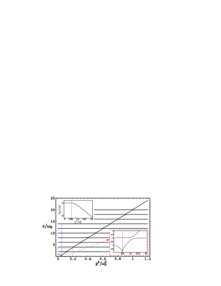
Figure 1: Energy spectrum for the discrete model; $N=10$ and $g_{k}=g\sqrt{\omega_{k}/2}$. The top-left inset shows the ground-state energy of the system. The bottom-right inset presents the area around the critical point, in which the first excited state collapses to the ground state. It also magnifies the anticrossing between the effective impurity level and the first field mode. In all the frames the vertical dashed line shows the quantum phase transition point.

When the field band is not bounded from above, except for the gradual effective cutoff, the impurity excitation level placed in the gap below the field band still undergoes the transition at the critical point, which is defined as $\alpha_{c}=\omega_{0}/4\Delta_{\textrm{eff}}$, and then merges with the field band. The split-off level above the band is not developed in this case.

Critical exponents. An important property of phase transitions is that systems with different microscopic dynamics behave equivalently at criticality. Their behavior depends only on the dimension of the system and the symmetry of the order parameter.Sachdev This phenomenon is known as universality. The parameters describing this critical behavior are universal quantities. Their behavior at the criticality is completely described in terms of a critical exponent.

Let us analyze the behavior of the lowest excited state energy (relatively to the ground state) in the vicinity of the critical point. We consider the discrete case first, factoring the magnitude of the interaction for convenience as $g_{k}\equiv g\,\chi_{k}$. Here $g$ is varied in the vicinity of the critical value $g_{c}=\sqrt{\omega_{0}}/\sqrt{4\sum_{k}\chi_{k}^{2}/\omega_{k}}$. This is feasible as far as the shape of the dependence stays the same. Stepping away form the critical point infinitesimally as $g=g_{c}\pm\delta g$, where the negative sign is taken for Eq.(7) and the positive for Eq.(12), one obtains

$$\varepsilon\sim N_{c}\left|g-g_{c}\right|^{z\nu}.$$ (14)

Here $z\nu=1/2$ is the critical exponent. The nonuniversal constant of proportionality which defines the energy scale from the left of the critical point is

$$N_{c}=\left(\frac{2\omega_{0}^{2}}{g_{c}+4\omega_{0}g_{c}^{3}\sum_{k=1}^{N}\chi_{k}^{2}\omega_{k}^{-3}}\right)^{1/2}.$$ (15)

After the critical point it is greater by a factor of $\sqrt{2}$. This behavior marks the second-order quantum phase transition.

In the case of continuously distributed field modes with the Ohmic model one varies $\alpha$ around the critical value $\alpha_{c}=\omega_{0}/4\Delta$ in Eq.(8) and (13), observing similar behavior for the impurity excitation energy

$$\varepsilon\sim N_{c}^{\prime}\left|\alpha-\alpha_{c}\right|^{z\nu},$$ (16)

with the same critical exponents $z=2$ and $\nu=1/4$. The nonuniversal coefficient $N_{c}^{\prime}$ to the left of the critical point is

$$N_{c}^{\prime}=\sqrt{\frac{4\omega_{0}\Delta}{1+\frac{\omega_{0}^{2}}{\Omega_{1}\Omega_{2}}}}\,.$$ (17)

After the critical point it acquires a factor of $\sqrt{2}$.

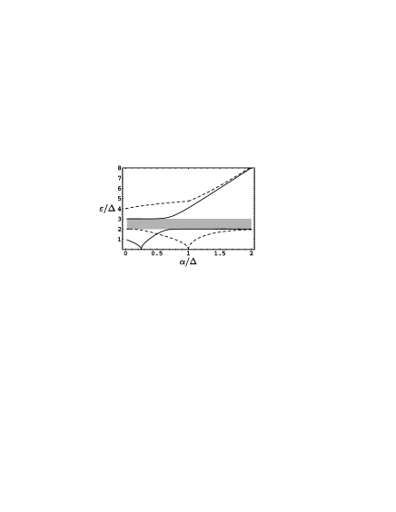
Figure 2: Energy spectrum for the continuous field distribution. The field band is shown by the shaded area. The solid curve represents the effective impurity excitation energy. It begins below the band at $\alpha=0$ and ends above the band at $\alpha\rightarrow\infty$ as purely atomic excitation energy. The quantum phase transition occurs when the first excitation energy of the system (solid bottom curve) hits the ground state at $\alpha_{c}=\Delta/4$. The ground-state energy changes similarly to the discrete case and is not shown here. The parameters are $\omega_{0}=\Delta$, $\Omega_{1}=2\Delta$, and $\Omega_{2}=3\Delta$. The dashed top curve shows the effective impurity when it is placed at $\omega_{0}=4\Delta$. In this case the quantum phase transition is manifested by the first exited level (bottom dashed curve) as it splits off below the band and hits the ground-state energy at $\alpha_{c}=\Delta$.

Entanglement as an order parameter.The quantum phase transition is governed by a divergent correlation length at the critical point. This is similar to what happens in the classical case. In the quantum case, though, there are correlations which do not have a classical analog. These purely quantum correlations are known as entanglement. It was demonstratedOsterloh ; Osborne ; Wu that there is a close relation between quantum phase transitions and entanglement. For a single-mode model it was shownEmary-QPT-Concurrence that the atoms become strongly entangled in the vicinity of the critical point. Osterloh et al.Osterloh have found that the concurrence is universal for the XY models. In what follows, we investigate the entanglement between the impurity atoms in the multimode field model and analyze how it is affected by the number of modes involved.

The entanglement of an effectively bipartite system can be measured by the concurrence,Concurrence which is a convex function of the entanglement of formation.Bennett For a given two-atom density matrix it is definedConcurrence as

$$C(\rho)=\max\Big{\{}0,2\max_{j}\lambda_{i}-\sum\limits_{j=1}^{4}\lambda_{j}\Big{\}},$$ (18)

where $\lambda_{j}$ are the eigenvalues of the Hermitian matrix $R=\sqrt{\sqrt{\rho}\widetilde{\rho}\sqrt{\rho}}$ and $\widetilde{\rho}=\left(\sigma_{y}\otimes\sigma_{y}\right)\rho^{*}\left(\sigma_{y}\otimes\sigma_{y}\right)$. Due to the symmetry of the atomic system with respect to the exchange of atoms, one can evaluate pairwise concurrence, extracting two-particle states from the multiparticle symmetric states. Wang and Mølmer have demonstratedWang-Molmer that the two-atom reduced density matrix written in the standard basis $\big{\{}\left|\uparrow\uparrow\right\rangle,\left|\uparrow\downarrow\right\rangle,\left|\downarrow\uparrow\right\rangle,\left|\downarrow\downarrow\right\rangle\big{\}}$ takes the form

$$\rho_{12}=\left(\begin{array}[]{cccc}v_{+}&x_{+}^{*}&x_{+}^{*}&u^{*}\\ x_{+}&w&y^{*}&x_{-}^{*}\\ x_{+}&y&w&x_{-}^{*}\\ u&x_{-}&x_{-}&v_{-}\end{array}\right).$$ (19)

As mentioned earlier, utilizing the symmetry of the atomic state under the exchange of particles one can express all the elements in Eq.(19)—i.e., the expectation values $\langle\sigma_{1i}\sigma_{2j}\rangle$, etc.—via the expectation values of the collective spin operators,Wang-Molmer

$$v_{\pm}\!\!\! = \!\!\frac{M^{2}-2M+4\left\langle J_{z}^{2}\right\rangle\pm 4\left\langle J_{z}\right\rangle\left(M-1\right)}{4M\left(M-1\right)},$$

$$x_{\pm}\!\!\! = \!\!\frac{\left(M-1\right)\left\langle J_{+}\right\rangle\pm\left\langle\left[J_{+},J_{z}\right]_{+}\right\rangle}{2M\left(M-1\right)},\,\,\,\,\,\,u\!=\!\frac{\left\langle J_{+}^{2}\right\rangle}{M\left(M-1\right)}$$

$$w\!\!\! = \!\!\frac{M^{2}-4\left\langle J_{z}^{2}\right\rangle}{4M\left(M-1\right)},\,\,\,\,\,\,y=\frac{2\left\langle J_{x}^{2}+J_{y}^{2}\right\rangle-M}{2M\left(M-1\right)}.$$ (20)

To calculate the above expectation values below and above the phase transition, we utilize Eq.(Quantum phase transition in the multimode Dicke model) in the limit of large $M$. Below the critical point we obtain

$$\left\langle J_{z}^{2}\right\rangle = \frac{M^{2}}{4}-M\left\langle b^{\dagger}b\right\rangle+\left\langle b^{\dagger}bb^{\dagger}b\right\rangle+{\cal O}(M^{-s}),$$

$$\left\langle J_{+}^{2}\right\rangle\!\! = \!\!\big{(}M-\sqrt{M}\big{)}\left\langle b^{\dagger}b^{\dagger}\right\rangle+{\cal O}(M^{-s}),$$

$$\left\langle J_{z}\right\rangle\!\! = \!\!-\frac{M}{2}+\left\langle b^{\dagger}b\right\rangle+{\cal O}(M^{-s}),\,\,\,\,s\geq 1/2.$$ (21)

The other expectation values are either trivial ($=0$) or can be derived from Eq.(Quantum phase transition in the multimode Dicke model). After the phase transition we have

$$\left\langle J_{z}^{2}\right\rangle^{\prime}\!\! = \!\!\frac{M^{2}}{4}\eta^{2}+\frac{M}{2}\left(1-\eta\right)+M\left(1-\eta\right)\left\langle b^{\dagger 2}\right\rangle^{\prime}$$

$$+ M\left(1-2\eta\right)\left\langle b^{\dagger}b\right\rangle^{\prime}+\left\langle b^{\dagger}bb^{\dagger}b\right\rangle^{\prime}+{\cal O}(M^{-s}),$$

$$\left\langle J_{+}^{2}\right\rangle^{\prime}\!\! = \!\!\frac{M^{2}}{4}\left(1-\eta^{2}\right)+\frac{M}{4}\left(\eta-1\right)+\frac{M}{2}\left(3\eta-1\right)\left\langle b^{\dagger 2}\right\rangle^{\prime}$$

$$+ \frac{3M}{2}\left(\eta-1\right)\left\langle b^{\dagger}b\right\rangle^{\prime}+{\cal O}(M^{-s}),$$

$$\left\langle J_{z}\right\rangle^{\prime}\!\! = \!\!-\frac{M}{2}\eta+\left\langle b^{\dagger}b\right\rangle^{\prime}+{\cal O}(M^{-s}),\,\,\,\,s\geq 1/2.$$ (22)

We point out that the ground states in Eqs. (Quantum phase transition in the multimode Dicke model) and (Quantum phase transition in the multimode Dicke model) are different, which is the reason for the “primes” in Eqs.(Quantum phase transition in the multimode Dicke model). Note also that after the critical point one has to include the shift of the bosonic operators in Eqs.(Quantum phase transition in the multimode Dicke model) to obtain Eqs.(Quantum phase transition in the multimode Dicke model).

The expectation values of the bosonic operators before the critical point are found utilizing the transformation (4) as $\langle b^{\dagger}b\rangle=\sum_{\beta}\overline{A}_{0\beta}^{2}$, $\langle b^{\dagger 2}\rangle=\sum_{\beta}A_{0\beta}\overline{A}_{0\beta}$, and $\langle b^{\dagger}bb^{\dagger}b\rangle=\sum_{\beta,\gamma}A_{0\beta}\overline{A}_{0\beta}A_{0\gamma}\overline{A}_{0\gamma}+\sum_{\beta,\gamma}\overline{A}_{0\beta}^{2}A_{0\gamma}^{2}+\sum_{\beta,\gamma}\overline{A}_{0\beta}^{2}\overline{A}_{0\gamma}^{2}$. Here we omit the complex conjugation since all the amplitudes are real. Together with Eqs. (LABEL:Eq:Solution-To-Direct-Transformation) and (7) these relations give the expectation values of the total spin operators. A similar procedure leads to the explicit expressions for the expectation values after the critical point (Quantum phase transition in the multimode Dicke model).

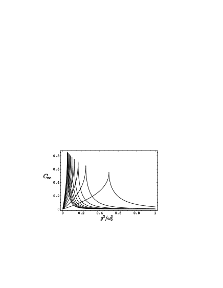
Figure 3: Concurrence for the discrete model with different numbers of field modes. From right to left, $N=1,2,\ldots,10$. The other parameters are the same as in Fig. 1.

For the Dicke model the reduced density matrix (19) simplifies, $x_{+}=x_{+}^{*}=x_{-}=x_{-}^{*}=0$, $y=y^{*}=w$, and the eigenvalues of the matrix $R$ are $\lambda_{1}=2w$, $\lambda_{2,3}=\big{|}u\pm\sqrt{v_{+}v_{-}}\big{|}$, and $\lambda_{4}=0$. One can verify that $\lambda_{2}>\lambda_{3}>\lambda_{4}>\lambda_{1}$, $u<\sqrt{v_{+}v_{-}}$, and $2w<u+\sqrt{v_{+}v_{-}}$. As a result the concurrence below and above the phase transition has the form $C=2(u-w)$. However, in the thermodynamic limit $M\rightarrow\infty$, the pairwise concurrence vanishes as $C={\cal O}(M^{-1})$ due to exchange symmetry, so we define the scaled concurrence Emary-QPT-Concurrence ; VidalConcurrence ; VidalCollective

$$C_{M}(\rho)=2M(u-w).$$ (23)

Using relations (Quantum phase transition in the multimode Dicke model), (Quantum phase transition in the multimode Dicke model), and (Quantum phase transition in the multimode Dicke model) and the expressions for $\langle b^{\dagger}b\rangle$, $\langle b^{\dagger 2}\rangle$, and $\langle b^{\dagger}bb^{\dagger}b\rangle$ we obtain the limiting value of the scaled concurrence, $C_{\infty}=\lim_{M\rightarrow\infty}C_{M}(\rho)$, in the form

$$C_{\infty}=\left(1+\theta\right)\sum_{\beta}W_{\beta}\frac{\omega_{0}-\varepsilon_{\beta}}{2\omega_{0}}+\frac{1}{2}\left(1-\theta\right)\,,$$ (24)

where

$$W_{\beta}=\left[1+\sum_{k}\frac{4g_{k}^{2}\omega_{0}\omega_{k}}{\left(\omega_{k}^{2}-\varepsilon_{\beta}^{2}\right)^{2}}\right]^{-1}.$$ (25)

Here $\theta\equiv 1$ below the critical point, $\gamma<\gamma_{c}$, and $\theta\equiv\eta$ above the critical point, $\gamma>\gamma_{c}$. Also we imply the replacements $\omega_{0}\rightarrow\widetilde{\omega}_{0}-2\zeta$, $g_{k}\rightarrow\widetilde{g}_{k}$ for $\gamma>\gamma_{c}$. In Fig. 3 we plot $C_{\infty}$ as a function of the coupling strength for various $N$, using the coupling constants in the form $g_{k}=g\sqrt{\omega_{k}/2}$ for an illustrative example. The concurrence reaches the maximum and breaks at the critical point. We note that the increase in the number of the field modes leads to the corresponding increase of the maximum bipartite entanglement in the atomic system.

Let us investigate the critical behavior of the concurrence. Introducing an infinitesimal deviation of the coupling from the critical point $g=g_{c}\pm\delta g$ one obtains $\delta C_{\infty}=-W_{0}^{c}\delta\varepsilon/\omega_{0}$ from the first term in Eq.(24). Here $W_{0}^{c}$ is $W_{0}$, [see Eq.(25)], evaluated at the critical point. As a result one has

$$C_{\infty}\sim-\frac{1}{\omega_{0}}W_{0}^{c}N_{c}\left|g-g_{c}\right|^{z\nu},$$ (26)

with the critical exponent $z\nu=1/2$, which defines entanglement (via concurrence) as an order parameter. One can easily generalize these results to the case of the continuum field model.

$A^{2}$-term. In many circumstances the overall Hamiltonian of the ensemble of two-state systems interacting with electromagnetic field would involve an additional field term.note1 One would expect a Hamiltonian of the form $H(t)=\sum_{j=1}^{M}[\mathbf{p}_{j}-\frac{e}{c}\mathbf{A}(t)]^{2}/2m+\sum_{j=1}^{M}V_{j}(\mathbf{r}_{j})$, where $\mathbf{p}_{j}$ and $\mathbf{r}_{j}$ are momentum and coordinate operators of the $j$th subsystem with confinement potential $V_{j}$. Rewriting the Hamiltonian in the eigenspace of the two-state systems with the assumptions discussed above we arrive at Eq.(1) with an additional term $M\frac{e^{2}}{2mc^{2}}\mathbf{A}^{2}$. In terms of the standard bosonic operators it is $\sum_{k}s_{k}(a_{k}^{\dagger}+a_{k})^{2}$ where $s_{k}$ depends on the density of states and therefore is finite when $M\to\infty$. Often this term is small with respect to the linear one and therefore is not considered. Nevertheless, it was shown Rzazewski ; Rzazewski2 ; Thompson1 ; Thompson2 that it can lead to the absence of the classical phase transition. Below we demonstrate that the quantum phase transition in the Dicke model with the $A^{2}$ term is present and can still be qualitatively described by the above results.

We consider a single-mode model with $\omega_{0}=\omega_{k}=\omega$. The diagonalization of Eq.(1) with the $A^{2}$ term—i.e., $s(a^{\dagger}+a)^{2}$—yields an expression for the spectrum in the form $\varepsilon^{2}=1+2s\pm\sqrt{(1+2s)^{2}-(1+4s-4g^{2})}$. Here $\varepsilon$, $s$, and $g$ are in units of $\omega$. Exactly as before, one finds the critical point at $g_{c}=\sqrt{1+4s}/2$, where the energy gap between the first excited and the ground state energy levels vanishes. Above this point the symmetry breaks. At the criticality the energy scales as $\varepsilon\to\sqrt{{4g_{c}}/(1+2s)}|g-g_{c}|^{1/2}$. After the critical point there is additional factor of $\sqrt{2}$ on the right-hand side. As a result, one observes the same transition with the same critical exponents and corrected position of the critical point.

In the multimode case the derivation is more cumbersome due to the cross terms in $\mathbf{A}^{2}$. Considering the above strategy it is expected that the generalization will yield similar unimportant corrections. We leave a thorough proof of this statement to be given elsewhere.

In summary, we investigated the model of the atomic ensemble interacting with an arbitrary discrete or continuous set of bosonic modes. The system was shown to undergo a quantum phase transition of the second order. In addition a series of anticrossing features following the criticality was revealed in the field band. Critical behavior of the parameters was found explicitly. It was demonstrated that the pairwise concurrence of the atomic system is broken at criticality with the same critical exponent as the energy.

- (1) R. H. Dicke, Phys. Rev. 93, 99 (1954).
- (2) K. Hepp and E. H. Lieb, Ann. Phys. (N.Y.) 76, 360 (1973).
- (3) F. T. Hioe, Phys. Rev. A 8, 1440 (1973).
- (4) G. Comer Duncan, Phys. Rev. A 9, 418 (1974).
- (5) K. Hepp and E. H. Lieb, Phys. Rev. A 8, 2517 (1973).
- (6) V. I. Emeljanov and Yu. L. Klimontovich, Phys. Lett. 59, 366 (1976).
- (7) K. Rza̧żewski, K. Wódkiewicz, and W. Żakowicz, Phys. Rev. Lett. 35, 1967 (1976).
- (8) K. Rza̧żewski and K. Wódkiewicz, Phys. Rev. A 13, 432 (1975).
- (9) B. V. Thompson, J. Phys. A 10, 89 (1977).
- (10) B. V. Thompson, J. Phys. A 10, L179 (1977).
- (11) S. Sachdev, Quantum Phase Transitions (Cambridge University Press, Cambrdge, England, 1999).
- (12) Y. K. Wang and F. T. Hioe, Phys. Rev. A 7, 831 (1973).
- (13) C. Emary and T. Brandes, Phys. Rev. Lett. 90, 044101 (2003).
- (14) M. Hillery and L. D. Mlodinow, Phys. Rev. A 31, 797 (1985).
- (15) J. Reslen, L. Quiroga, and N. F. Johnson, Europhys. Lett. 69, 8 (2005).
- (16) J. Vidal and S. Dusuel, Europhys. Lett. 74, 817 (2006).
- (17) G. Liberti, F. Plastina and F. Piperno, Phys. Rev. A 74, 022324 (2006).
- (18) V. Privman, in Finite Size Scaling and Numerical Simulation of Statistical Systems, edited by V. Privman (World Scientific, Singapore, 1990), p. 1.
- (19) N. Lambert, C. Emary, and T. Brandes, Phys. Rev. Lett. 92, 073602 (2004).
- (20) H. W. Chan, A. T. Black, and V. Vuletic, Phys. Rev. Lett. 90, 063003 (2003).
- (21) S.-Y. Lin, J. G. Fleming, M. M. Sigalas, R. Biswas, and K. M. Ho, Phys. Rev. B 59, R15579 (1999).
- (22) A. Kiraz, P. Michler, C. Becher, B. Gayral, A. Imamoglu, L. Zhang, E. Hu, W. V. Schoenfeld, P. M. Petroff, Appl. Phys. Lett. 78, 3932 (2001).
- (23) M. Keller, B. Lange, K. Hayasaka, W. Lange, and H. Walther, Nature (London) 431, 1075 (2004).
- (24) T. Holstein and H. Primakoff, Phys. Rev. 58, 1098 (1949).
- (25) A. J. Leggett, S. Chakravarty, A. T. Dorsey, M. P. A. Fisher, A. Garg, and W. Zwerger, Rev. Mod. Phys. 59, 1 (1987).
- (26) A. Osterloh, L. Amico, G. Falci, and R. Fazio, Nature (London) 416, 608 (2002).
- (27) T. J. Osborne and M. A. Nielsen, Phys. Rev. A 66, 032110 (2002).
- (28) L.-A. Wu, M. S. Sarandy, and D. A. Lidar, Phys. Rev. Lett. 93, 250404 (2004).
- (29) W. K. Wootters, Phys. Rev. Lett. 80, 2245 (1998); S. Hill and W. K. Wootters, ibid. 78, 5022 (1997).
- (30) C. H. Bennett, D. P. DiVincenzo, J. A. Smolin, and W. K. Wootters, Phys. Rev. A 54, 3824 (1996).
- (31) X. Wang and K. Mølmer, Eur. Phys. J. D 18, 385 (2002).
- (32) J. Vidal, G. Palacios, and R. Mosseri, Phys. Rev. A 69, 022107 (2004).
- (33) J. Vidal, Phys. Rev. A 73, 062318 (2006).
- (34) The corrections for phonon fields may be more complicated.