Lattice Model of Sweeping Interface for Drying Process in Water-Granule Mixture

Abstract

Based on the invasion percolation model, a lattice model for the sweeping interface dynamics is constructed to describe the pattern forming process by a sweeping interface upon drying the water-granule mixture. The model is shown to produce labyrinthine patterns similar to those found in the experiment[Yamazaki and Mizuguchi, J. Phys. Soc. Jpn. 69 (2000) 2387]. Upon changing the initial granular density, resulting patterns undergo the percolation transition, but estimated critical exponents are different from those of the conventional percolation. Loopless structure of clusters in the patterns produced by the sweeping dynamics seems to influence the nature of the transition.

1 Introduction

During drying process, it often happens that material dispersed in fluid condenses and leaves patterns on a substrate[1]. A typical one is dry stain made by coffee spilt over a table. Yamazaki and Mizuguchi demonstrated[2] that the water-granule mixture that is confined in the narrow gap between two glass plates produces much more complicated patterns than coffee stain upon drying; Labyrinthine patterns of granules emerge as granules are swept by one-dimensional water-air interfaces as they recede during the drying process.

Physical processes are as follows; As the water evaporates from the gap between the plates, the volume of the wet region tends to shrink and the pressure in the water decreases, which gives the driving force to move the interface between the water and the air; Although the pressure difference should be almost uniform over the whole interface, the interface does not move uniformly, but only the weakest part moves at a time. As the interface moves, it sweeps the dispersed granules to collect them along it; Consequently, the interface becomes more difficult to move due to the friction of granules with the glass plates. At some parts of the interface, the granular density eventually exceeds the threshold where granules get stuck to form a pattern after drying.

For this phenomenon, several models have been proposed. In their original paper on the experiment, Yamazaki and Mizuguchi analyzed the elementary process to estimate the thickness of the granule region assuming the granular region as elastic material[2]. A phase field model with the granular density field[3, 4] and the boundary dynamics[5] have been constructed, based on the observation that the sweeping phenomenon can be regarded as the small diffusion limit of the crystal growth[6, 7].

In this paper, focusing on similarities in dynamics between the sweeping process described above and the invasion percolation[8], we present a simple lattice model of sweeping interface for pattern formation. We performed numerical simulation on the model and analyzed the resulting patterns.

2 Lattice Model of Sweeping Interface

The model consists of two variables at each site of the triangular lattice: the state variable $s_{i}$ and the granular density $f_{i}$ on the site $i$. The state variable $s_{i}$ takes the values either 0 or 1 depending upon whether the site $i$ is dry or wet:

$$s_{i}=\left\{\begin{array}[]{ll}0&\mbox{(if the site $i$ is dry)}\\ 1&\mbox{(if the site $i$ is wet)}\end{array}\right..$$ (1)

The granular density $f_{i}$ takes zero or a positive real number representing the quantity of granules in the $i$’th cell.

Initially, all the sites in the system are wet and the granules are distributed uniformly with some randomness, thus the initial value of the state variables $s_{i}$’s are 1 for all the sites, and the granule density $f_{i}$’s are given random values from the uniform distribution with the width $\Delta f$ and the upper bound $f_{M}$: $f_{i}\in[f_{M}-\Delta f,f_{M}]$.

The interface site is defined as a wet site adjacent to a dry site. We assume the sites outside of the system are dry, thus the wet regions are surrounded by the one dimensional chains of the interface sites, which we call the interface.

Upon drying, the water volume shrinks, then the pressure decreases in the water region. The pressure difference between the wet and the dry regions pushes the interface toward the wet region, but the site that actually moves is the least resistive site. The resistance, or the strength of the interface sites, against the interface motion is determined by the granular density $f_{i}$ and the local configuration of interface; The granules causes friction with the glass plates, while the interface sites surrounded by the dry sites are easier to dry due to the surface tension that tends to make the interface straight. In order to take these effects in a simple way, we introduce the strength $r_{i}$ of the interface site $i$ as a function of its granular density $f_{i}$ and the number of neighboring dry sites $n_{i}$. We employ the simple form

$$r_{i}=\left\{\begin{array}[]{ll}f_{i}&\mbox{if }n_{i}<n_{s}\\ f_{i}-\gamma&\mbox{if }n_{i}\geq n_{s}\end{array}\right.$$ (2)

with two parameters $\gamma$ and $n_{s}$, which represent the surface tension effect.

Sweeping of granules takes place when the interface moves; Upon drying a wet interface site, the granules on this dried site are swept away to the neighboring wet sites, as long as the granular density of the site is not high enough for the granules to get stuck. If the granule density exceeds a threshold value $g_{\rm th}$, the granules get stuck between the glass plates and cannot move, thus they stick to the sites and form a pattern after the whole system is dried.

To represent the above processes, the dynamics for the lattice model of the sweeping interface is defined as follows. (i) Out of the sites with $f_{i}<g_{\rm th}$, pick the weakest interface site $i$, whose strength $r_{i}$ is smallest. If all the interface sites have $f_{i}\geq g_{\rm th}$, then pick the weakest site from them. (ii) Dry the site $i$ by changing its state variable $s_{i}$ from 1 to 0. (iii) Redistribute $f_{i}$ to the neighboring wet sites equally if $f_{i}$ is smaller than $g_{\rm th}$ and there exist some wet neighbor sites; Otherwise do nothing. Repeat the steps (i) – (iii) until all the sites becomes dry.

There are five parameters that characterize the model: $\Delta f$ and $f_{M}$ to characterize the initial distribution of granular density, $\gamma$ and $n_{s}$ to control the effect of surface tension on the interface motion, and $g_{\rm th}$, that is the upper limit for the sweeping to take place. Out of four parameters, $\Delta f$, $f_{M}$, $\gamma$, and $g_{\rm th}$, we can eliminate one that sets the scale for the granular density; We take $g_{\rm th}=1$.

In the following simulations, we fix the parameter $\Delta f$ to be $0.5f_{M}$ for simplicity, and take $n_{s}=3$, i.e. half of the number of neighboring sites in the triangular lattice that we are using. Then we have only two parameters, $f_{M}$ and $\gamma$.

3 System behavior

3.1 Patterns and surface tension effects

Figure 1: Patterns produced by the sweeping interface model with and without the surface tension effect ($\gamma=0$ for the left column and $\gamma/g_{th}=1$ for the right column). The sites with the granules are represented by the solid circles whose sizes are proportional with the granule density. The initial granular density is given by $f_{M}=0.1$(the top row), 0.5(the middle row), and 0.9(the bottom row) with $\Delta f=0.5f_{M}$ and $n_{s}=3$. The linear system size is $L=64$.

First, we compare the patterns for $\gamma/g_{\rm th}=0$ with those for $\gamma/g_{\rm th}=1$ in order to examine the surface tension effects in Fig.1, where the sites with granules are represented by the solid circles whose sizes are proportional to the density. The initial grain densities are given by $f_{M}/g_{\rm th}=0.1$, 0.5, and 0.9, and the system size $L\times L$ with $L=64$. One can see the surface tension effects especially in the lower density cases; The grains tend to align in the systems with the surface tension $\gamma/g_{\rm th}=1$ for $f_{M}=0.1$. These correspond to the patterns obtained in the experiment[2]. In the higher density cases, the surface tension effect is small. In the rest of the paper, we study only the case of $\gamma/g_{\rm th}=1$ and change $f_{M}$.

Note that, in the case of $\gamma/g_{th}=1$, the pattern consists of winding paths delineated by walls of granular sites; the width of the paths are proportional to $1/f_{M}$, while that of the walls is always of order of one lattice site because we assume that granules are swept only to the neighboring sites in the present model.

3.2 Invading process

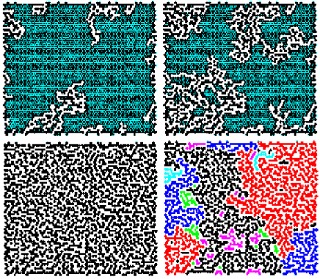
Figure 2: (Color online) Time development and final patterns. The upper two plates show the drying process. The blue regions denote the wet regions. The lower left plate shows the final pattern after drying with the granule density represented by the solid circles. The lower right plate shows the cluster structure of the same pattern. The parameters are $f_{M}/g_{th}=0.871$, $\Delta f=0.5f_{M}$, $n_{s}=3$, $\gamma/g_{th}=1$ and $L=64$.

Fig.2 shows time development of the drying process for $f_{M}/g_{\rm th}=0.871$ for the system with $L=64$. While one site is dried at each time step, the spatial development is not homogeneous but intermittent as in the case of the invasion percolation model. The difference in the pattern from the invasion percolation model is that the invaded (or dried) region develops a winding path structure, and the basic mode of development is extending narrow paths. This is due to the sweeping process, by which the granules on a dried site are swept away to the adjacent wet sites; This makes walls on both sides of the path, consequently, it is easier to advance ahead making a narrow path than to widen the swept region beyond a certain width. This path extending process leads to a labyrinthine pattern of granules when the drying process is completed.

Both of the two plates in the lower row of Fig.2 represent the same pattern obtained by this process; The lower left plate shows the grain density distribution by solid circles whose size is proportional to the density. The pattern consists of strings of the sites with grains. If we define a cluster as a set of connected sites with non-zero grain density, the whole pattern can be decomposed into clusters; In the lower right plate of Fig.2, its cluster structure is shown by coloring. The clusters are of highly branched structure, but there are virtually no loops of granular sites; The shape of clusters is compact and their fractal dimension appears to be very close to two. One can see that one of the clusters is percolating from the top to the bottom; In this case, we call the system percolated.

4 Percolation transition of the sweeping interface model

In the following, we will examine the percolation transition in the pattern produced by the sweeping interface model.

4.1 Occupation ratio

Figure 3: (a) Proportion of occupied sites $p$ vs. $f_{M}$ for the system size $L=256$. (b) The percolation probability $\Pi$ vs. the occupation proportion $p$ for various system sizes $L$. The system sizes are $L=$124, 256, 512, 1024, 2048, 4096, and 8192 from the left curve to the right. The lines denote the fitting function by the error functions with $p_{50}(L)$ and $\Delta p$ (see text). Each plot represents average over $200\sim 1000$ realizations. The vertical line is drawn at $p=p_{c}=0.5221$. (c) $p_{50}(L)-p_{c}$ and $\Delta p$ vs. $L$ in the logarithmic scale. $p_{50}(L)-p_{c}$ is plotted with $p_{c}=0.5221$ in the left scale and $\Delta p$ in the right scale. The solid lines represent the lines with the slope $-0.50$. The other parameters of the model are $\Delta f=0.5f_{M}$, $\gamma/g_{th}=1$, and $n_{s}=3$.

The proportion $p$ of the sites with grains after drying is not an input parameter but is obtained by performing simulations with the initial distribution given by $f_{M}$. In Fig.3(a), $p$ is plotted against $f_{M}/g_{\rm th}$. The plot is for the system with $L=256$, but the size dependence is small when $L$ is larger. The ratio $p$ is an almost linearly increasing function of $f_{M}/g_{\rm th}$, but one can see a small bump near $f_{M}/g_{\rm th}\approx 0.9$, or $p\approx 0.5$; This roughly corresponds with the percolation transition point. We will not pursue this any further in this paper although we do not understand its nature yet.

4.2 Percolation probability

Fig.3(b) shows the percolation probability $\Pi$ as a function of $p$ for various lattice size $L$. The lines show fitting curves by the error function as

$$\Pi(p;L)={\rm Erf}\Bigl{(}(p-p_{50}(L))/\Delta p(L)\Bigr{)},$$ (3)

where the error function is defined by

$${\rm Erf}(x)\equiv\frac{1}{\sqrt{\pi}}\int_{-\infty}^{x}e^{-t^{2}}dt;$$ (4)

$p_{50}(L)$ is the occupied site proportion where $\Pi=0.5$, and $\Delta p(L)$ is the width of the percolation transition for the finite system of the size $L$. For lower granular density, the system is not percolated, while the percolation probability is almost one at higher density; The curve is steeper, or $\Delta p(L)$ is smaller, for the larger system, which suggests that there exists a sharp transition at a finite density in the infinite system size limit as in the case of the conventional percolation problem.

In comparison with the conventional percolation, the difference is in the $L$ dependence of $\Pi(p;L)$; $\Pi(p;L)$ is a decreasing function of $L$, therefore, there is no fixed point where the percolation probability $\Pi$’s for all $L$ intersect.

As $L$ becomes large, $p_{50}(L)$ converges to a finite value $p_{c}$ and $\Delta p(L)$ goes to zero as

$$p_{c}-p_{50}(L) \sim L^{-1/\nu_{1}}$$ (5)

$$\Delta p(L) \sim L^{-1/\nu_{2}}$$ (6)

with the exponents $\nu_{1}$ and $\nu_{2}\approx 1/0.50$, and the threshold $p_{c}\approx 0.5221$ (Fig.3(c)). The corresponding value of $f_{M}$, or $f_{c}$, is $f_{c}/g_{\rm th}\approx 0.926$. The fact that $\nu_{1}\approx\nu_{2}$ suggests that there is a unique length scale $\xi$, which diverges as

$$\xi\sim|p-p_{c}|^{-\nu}$$ (7)

with the exponent $\nu\approx 2.0$. Note that its value 2.0 is quite different from 4/3, or the value for the 2-d percolation[9].

4.3 Order parameter

Figure 4: (a) The order parameter $P$ vs the occupation ratio $p$ for $L=64\sim 8192$. The vertical line is drawn at $p=p_{c}=0.5221$. (b)The scaling plot with $\beta=0.02$ and $\nu=2.0$.

The percolation order parameter $P$, or the ratio of the sites that belongs to the percolating cluster, is shown in Fig.4(a) for $L=64\sim 8192$. The value of $P$ at $p=p_{c}$ is almost independent of $L$, thus the transition looks first order, but one can observe slight tendency of decrease in $P$ at $p=p_{c}$ for the systems $L>1024$, which implies the transition is of the second order with a small value of the exponent $\beta$;

$$P(p)\sim(p-p_{c})^{\beta}.$$ (8)

The scaling plots

$$P(p;L)=L^{-\beta/\nu}f_{P}\Bigl{(}(p-p_{c})L^{1/\nu}\Bigr{)}$$ (9)

with the scaling function $f_{P}(x)$ are shown in Fig.4(b) with $\beta=0.02$ and $\nu=2.0$. The plot looks reasonably good, but one may find some scatter.

4.4 Cluster size distribution

Figure 5: The cluster size distributions below (a), at (b), and above (c) the percolation transition for various system sizes. The initial granular density is given by $f_{M}=0.88$(a), 0.926(b), and 0.95(c) with the resulting $p\approx 0.502$(a), 0.522(b), and 0.531(c). The system sizes are $L=32\sim 1024$ (a), $128\sim 4096$ (b), and $128\sim 1024$ (c). The other parameters are $\Delta f=0.5f_{M}$, $\gamma/g_{th}=1$ and $n_{s}=3$.

The cluster size distribution $n(s)$ is introduced as the number of clusters with the size $s$ divided by the number of lattice sites $L^{2}$ in the system, thus it is normalized as

$$\sum_{s=1}^{L^{2}}s\,n(s)=p.$$ (10)

In Fig.5, the cluster size distributions are shown in the logarithmic scale for $p<p_{c}$ (a), $p\approx p_{c}$ (b), and $p>p_{c}$ (c). In the case of $p<p_{c}$ (a), the distribution has finite width in the large $L$ limit. As for the case of $p>p_{c}$ (c), it is also of finite width but with an isolated peak for each system size; The peak corresponds with the percolating clusters. The distribution at $p\approx p_{c}$ in Fig.5(b) is intriguing; They show the power law distribution

$$n(s)\sim s^{-\tau}$$ (11)

with the exponent $\tau=2.25$, but there are peaks at the large cluster end of the distribution; The position of the peak scales with almost $L^{2}$ which suggests they corresponds to the percolating cluster. This is consistent with the result of percolation probability in Fig.3(b), which shows the system with any finite size is percolating at $p=p_{c}$.

Figure 6: The scaling plot of the cluster size distribution at the percolation transition $p=0.5221$ ($f_{M}=0.9259$) for $L=128\sim 8192$. (a) The data for $s\geq 4$ are plotted with $D=2$ and $\tau=2.25$. (b) The data that correspond to the percolating clusters are removed in the plot with $D^{\prime}=1$ and $\tau=2.25$, using the same scaling form (12). The solid lines indicate the line with the slope $-2.25$.

Fig.6 shows the scaling plot

$$n(s;L)=L^{-D\tau}f_{n}(s/L^{D})$$ (12)

at $p\approx p_{c}$ for $D=2$ (a) and 1 (b) with $\tau=2.25$ for the both.

From Fig.6(a) with $D=2$, one can see the peak position scales with the system area. This is consistent with the observation that the percolating clusters look compact and two-dimensional in Fig.2. If one looks carefully, however, one may find systematic deviation near the peak. This can be interpreted as the distribution deviates from the power law (11) at $s>s_{c}(L)$, and $s_{c}(L)$ does not scale as $L^{2}$ but $L^{D^{\prime}}$ with another exponent $D^{\prime}$.

To see this, we plot the same data except for the two data points that correspond to the large percolating clusters for each $L$; We tried various values of $D^{\prime}$, but $D^{\prime}=1$ seems to give least scatter around the master curve(Fig.6(b)). The fact that $D$ and $D^{\prime}$ are quite different simply means that the boundary effect has strong influence on the cluster distribution, but the exponent $D^{\prime}$ should not be associated with the fractal dimension of the geometrical structure of clusters.

5 Discussions and summary

	$\nu$	$\beta$	$\tau$	$D$
sweeping interface model	2.0	0.02	2.25	2.0
2-d percolation	3/4	5/36	187/91	91/48

Table 1: The critical exponents at the percolation threshold for the sweeping interface model and the conventional 2-d percolation[9].

The exponents obtained above are listed with those for the two-dimensional conventional percolation transition(Table 1); They are clearly different, suggesting that the nature of the transition is different from that of the conventional percolation. This may not be very surprising because the labyrinthine patterns analyzed here are results of the dynamical process of sweeping, which could induce long range correlation, while the conventional percolation transition is for the pattern by random deposition.

Most remarkable difference, however, is the behavior of the percolation probability $\Pi(p;L)$ in Fig.3(b). For the sweeping interface model, the $\Pi(p;L)$ is a decreasing function of $L$ for any $p$, thus $\Pi(p;L)$’s for different $L$ do not intersect, while those for the percolation intersect at $p=p_{c}$. This feature, however, may be explained by the fact that the clusters produced by the sweeping dynamics have branching structure with virtually no loops; Even in a very large cluster, the path that connects any given two sites in the cluster is essentially unique[10], thus, for a fixed $p$, the percolating cluster is more difficult to appear in a larger system because breakage of a path at any site during drying process may break the cluster apart. One consequence of this feature is that the finite system is almost always percolated at the percolation threshold $p=p_{c}$ for the infinite system.

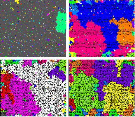
Figure 7: (Color on line) Cluster structure at the percolation threshold $p=0.522$. The cluster structure of the whole system of the size $L=1024$ (upper left), and its subsets at the central part of the size 512 (upper right), 256 (lower left), and 128 (lower right) are shown.

Another aspect of the loopless structure of cluster is that the cluster structure of the system changes drastically when the system is trimmed. Fig.7 shows the cluster structure of the system with $L=1024$ and its subsystems for $p\approx p_{c}$. The upper left plate is the original system of $L=1024$. The largest percolating cluster colored by grey is dominating the system. The upper right, lower left, and lower right plates show the central parts of the original system of the size $L=512$, 256, and 128, respectively. The cluster structure are analyzed only within the subsystems, i.e. the clusters that are connected only outside of the subsystems are disconnected in the subsystem. One can see there are no percolating clusters in the smallest subsystem because the original percolating cluster is fragmented into small pieces when we look at only a smaller part of it. This should be a general feature for the labyrinthine structure; There is virtually no loop in clusters, therefore, there is usually only one connecting path between any two sites in a cluster. Consequently, clusters are easily fragmented into pieces when they are trimmed to fit into a smaller part of the system.

This may pose some problems in the analysis of experimental data; In the experiment, it should be difficult to analyse whole systems because the regions near the boundary are usually disturbed. In the finite size scaling analysis, the samples with smaller sizes are generated by trimming larger samples[2], but the present analysis suggests that such a procedure changes the cluster structure and results may well depend upon the size of the original system.

In summary, being stimulated by the labyrinthine pattern produced in the drying process, we have constructed the lattice model of the sweeping interface based on the invasion percolation, and demonstrated the model produces similar patterns. The cluster analysis of the resulting patterns shows that there is a percolation transition upon changing the density in the initial state, but the loopless structure of the labyrinthine patterns obtained by the sweeping dynamics make the nature of the transition different from the conventional percolation.

The authors thank Dr. Yamazaki for showing unpublished experimental data. This work is partially supported by a Grant-in-Aid for scientific research (C) 16540344 from JSPS.

References

- [1] R.D. Deegan, Phys. Rev. E 61 (2000) 475.
- [2] Y. Yamazaki and T. Mizuguchi, J. Phys. Soc. Jpn. 69 (2000) 2387.
- [3] Y. Yamazaki, M. Mimura, T. Watanabe, and T. Mizuguchi, unpublished.
- [4] T. Iwashita, Y. Hayase, and H. Nakanishi, J. Phys. Soc. Jpn. 74 (2005) 1657.
- [5] H. Nakanishi, arXiv: cond-mat/0508622, to be published in Phys. Rev. E (2006).
- [6] For review, see for example, J.S. Langer, Rev. Mod. Phys. 52 (1980) 1.
- [7] W.W. Mullins and R.F. Sekerka, J. Appl. Phys. 34 (1963) 323; ibid. 35 (1964) 444.
- [8] D. Wilkinson and J.F. Willemsen, J. Phys. A 16 (1983) 3365.
- [9] D. Stauffer and A. Aharony, “Introduction to Percolation Theory” 2nd edition, Taylor and Francis, 1994.
- [10] Large loops may appear for the case where the average initial granular density is greater than , but near the percolation transition threshold, there exist only small loops if any, because, in order that a large loop is to appear, a large area should be surrounded by the interface sites whose granular densities are all greater then or equal to .