Permeability up-scaling using Haar Wavelets

Abstract.

In the context of flow in porous media, up-scaling is the coarsening of a geological model and it is at the core of water resources research and reservoir simulation. An ideal up-scaling procedure preserves heterogeneities at different length-scales but reduces the computational costs required by dynamic simulations. A number of up-scaling procedures have been proposed. We present a block renormalization algorithm using Haar wavelets which provide a representation of data based on averages and fluctuations.

In this work, absolute permeability will be discussed for single-phase incompressible creeping flow in the Darcy regime, leading to a finite difference diffusion type equation for pressure. By transforming the terms in the flow equation, given by Darcy’s law, and assuming that the change in scale does not imply a change in governing physical principles, a new equation is obtained, identical in form to the original. Haar wavelets allow us to relate the pressures to their averages and apply the transformation to the entire equation, exploiting their orthonormal property, thus providing values for the coarse permeabilities.

Focusing on the mean-field approximation leads to an up-scaling where the solution to the coarse scale problem well approximates the averaged fine scale pressure profile.

¹Department of Earth Science and Engineering, ²Department of Physics, Imperial College London, United Kingdom

1. Introduction

The term up-scaling is used in reservoir engineering to refer to the procedure by which a geological model is coarse grained into a flow model. This is essential in modelling mass transport correctly to gain an understanding of subsurface systems such as oil fields, ground water flow and waste deposits. Correct estimation of the transport properties of these reservoirs, including permeability, is vital for their management. For example, in the contexts mentioned above, good control of the fluid dynamics is necessary to ensure optimization of recovery and the safety of the environment [Noet:futurestoch, ]. The procedure presented in this paper, based on renormalization and wavelets, is a general coarse graining technique, inspired by the wavelet treatment of the Ising model and in line with the new developments that have been suggested in the field of materials modelling Ism:W2005 ; Ism:W .

In Section 1.1, the main up-scaling methods and related issues will be briefly reviewed. In Section 2 a short account of real-space renormalization and Haar wavelets will be given leading to the description of the proposed method in Section 3. Numerical simulations and results will be presented in Section 4.

The present paper is intended as a proof of concept of how wavelets can be used in the field of upscaling by establishing a specific formalism and applying it to the simplest cases. This allows us to explore the underlying workings of the method, an essential step towards the treatment of less trivial problems.

1.1. Up-scaling techniques

Numerous methods have been suggested for the coarsening of permeability in geological systems, the simplest being averaging techniques. As highlighted in a classic review [Farmer:krev, ], we can subdivide up-scaling methods into three categories: deterministic, stochastic and heuristic. Further distinctions can be made between analytical and numerical methods. The main issue with up-scaling is the heterogeneity which characterizes natural porous media on many different length scales. Heterogeneities range from millimeters to kilometers, due to the great variety of types of rocks and depositional processes that can be present in the same system. Often, there is no clear division between the system size and the length scales of the features or the size of the cells in the model.

An analogy can be made between flow in porous media and currents through resistors. This is possible because of the nature of the equation for flow, Darcy’s law, which is an elliptic equation relating flow to the gradient of the pressure just like Ohm’s law relates current to voltage drop in conductors.

The problem of up-scaling is thus translated into solving the Laplace-like differential equation, encouraging the application of the wide range of methods which have been devised for this purpose in other fields, for example field theoretical techniques, perturbation expansions, effective medium theory, percolation approaches or more simply finite differences and finite elements methods, see Ref. [Farmer:krev, ] for a recent review. A serious drawback of these techniques, especially perturbation and effective medium theory, is the underlying assumption that fluctuations in permeability are small.

Renormalization offers an alternative, allowing for large fluctuations in the system to be taken into account. Renormalization techniques are a step-by-step approach where the system is coarsened progressively, integrating out features on small length scales, leading to the large scale effective permeability. Moreover, renormalization can be applied to stochastic data sets by acting on the probability distribution of the considered property rather than on the single data points Hast:permup .

With the exception of geological modelling techniques involving object based methods and irregular grids, typically permeability data is interpolated stochastically from the information gained at precise locations in the reservoir. Hence, the emphasis is on preserving the features of its statistical distribution rather than the precise values. Furthermore, uncertainty pervades all stages of reservoir modelling, from the measurement of permeability to the estimation of the size of different rock type elements, rendering statistical analysis the only viable tool to account for a range of equiprobable scenarios which could represent the physical system Chris:errors .

Although there are various solutions to calculating effective permeability for specific conditions, most of them have not been implemented in the standard reservoir engineering packages for industry. In practice, the methods of choice are often simple averages, due to the ease and speed with which they can be implemented and to the fact that precision in the estimation of permeability in a specific location does not affect the uncertainty implicit in the modelling process.

2. Renormalization and Haar Wavelet Transforms

2.1. Renormalization in up-scaling

The concept of real-space renormalization has proved to be extremely useful in estimating effective permeability efficiently [King:renkeff, ]. The basic idea behind this method is to start with a lattice on which a property, in this case permeability, is defined at each lattice cell. Successively the original cells are grouped in a number of blocks, assigning new values for the coarsened property. To avoid confusion, it is necessary to clarify what is referred to by the words “block” and “cell”. A cell is the basic unit of the fine grid which typically characterizes the geological model. Cell permeability is therefore what is commonly referred to as fine permeability. A block is the basic unit of the coarse grid used in flow simulations. The term block permeability refers to the coarse equivalent permeability of the block, calculated from the cell permeabilities through up-scaling Wen:condrev . This is clearly dependent on the boundary conditions and is different from effective permeability, defined as the permeability needed to relate the mathematical expectations of the flow and of the pressure gradient. Due to the finite size of the blocks it is only possible to consider equivalent permeability, which ensures a match of flow patterns between the block and the constitutive cells. After rescaling all the length scales, blocks become cells and the result is a coarse-grained lattice with fewer cells, but which still possesses the essential features of the original system.

This procedure was first suggested by Kadanoff:blockspins as an efficient method to extrapolate the large scale behaviour of an infinite system once fluctuations on smaller scales are averaged out. The main advantage is that the procedure can be repeated until the lattice has achieved the required coarseness with a low computational cost, the algorithm being linear in the system size.

The renormalization transformation is by no means unique and many different renormalization schemes have been proposed, some inspired by an analogy between flow in porous media, percolation processes and the flow of currents through resistors Will:Mathsoilren .

Real-space transformations are a particular case of the more general concept of the renormalization group. While the real-space version already provides a versatile and fast technique for up-scaling, a “full” real- and momentum-space renormalization method for coarse-graining of subsurface reservoirs was presented by Hristopoulos et al. hrist:RGoverview ; hrist:RG1999 . This general treatment has confirmed the applicability of the renormalization concept to up-scaling, providing a solution of the problem in all orders of perturbation, even for heterogeneous systems where large fluctuations render other methods unsound.

2.2. The Haar wavelet transform

The mathematical concept of wavelets was first suggested in 1909 by Haar Haar:wav . It found its first application in the field of seismology in 1989 in the work of Morlet Morelt:wav and has since then been at the origin of a substantial number of new approaches to various subjects, for example, biology Wav:bio and statistical mechanics Ism:W . The basic idea underlying wavelets is to decompose a function or a set of data, in the continuous and discrete case respectively, into basic components and their relative coefficients Daubechies:10lec . In this sense it is very similar to a Fourier transform, where the basic components are sines and cosines and the coefficients are given by their amplitude. Wavelet transforms, however, offer both spatial and frequency resolution. For this reason they have been particularly successfully applied to the analysis of signals where it is necessary to capture both underlying periodic functions and specific localized features, which are almost impossible to represent with periodic components.

At this point, however, a distinction between two different uses of wavelets must be made. On one side, wavelets can be used to compress information in terms of reducing the number of data points with a filtering procedure. This has been applied extensively in the context of up-scaling by Sahimi Sahimi:swa2004 , where a filtering process reduces the number of permeability values in the system without compromising its general statistics. On the other side, a more “pervasive” application of wavelets can lead to the coarsening of permeability by acting on the flow equations themselves. This approach has been suggested in statistical physics to compress the information relative to spins and coupling constants in the Ising model Ism:W and then extended to include various aspects of materials modelling Ism:W2005 .

The main point, already noted by Best Best:LandauGins , is that there is a striking similarity between the perspective of renormalization and of wavelet transforms: both highlight the features of a system in terms of large scale behaviour and fluctuations away from it and both provide a connection between the different relevant scales.

In this paper, the simplest type of discrete wavelet transform, the Haar transform, is implemented in a renormalization method. Its effect is to separate the average of the original data from the fluctuations, expressed in terms of differences. Wavelets are constructed through the scaling and shifting of the so called mother wavelet.The Haar wavelet is defined as follows, Daubechies:10lec : $\psi_{jk}\left(x\right)\equiv\psi\left(2^{j/2}x-k\right)$, where $\psi\left(x\right)$ is the mother wavelet, $j\in z$ is the scale parameter and $k$ is the shift. This leads to a Haar wavelet matrix of the form:

$$\mathbf{H}=\left[\begin{array}[]{cc}1&\phantom{-}1\\ 1&-1\end{array}\right].$$

For example, if we apply this transform to a $2\times 1$ vector we can obtain a new vector in terms of sums and differences of the original values. As will be seen in Section 3 this is a useful up-scaling scheme valid in any dimension. This is a very simple transform, however, the formalism described can be easily applied with any matrix transform.

2.3. The system: single-phase laminar flow

The simple problem analysed in this paper is single-phase creeping flow of a viscosity dominated incompressible fluid through a porous medium. We will assume unit viscosity and ignore the effect of gravity. The basic equation is Darcy’s equation for flow, $\mathbf{q=-K\nabla P}$, where $\mathbf{K}$ is permeability and $\mathbf{\nabla P}$ is the gradient of pressure, combined with the continuity equation, $\mathbf{\nabla\cdot q}=0$, which give rise to a Laplace-like differential equation: $\mathbf{\nabla}\cdot(\mathbf{K\nabla P})=0$.

The discretization was performed by specifying the permeability values at the cell centres and assuming pressure to be piece-wise linear across the cell. Transmissibility is equal to permeability in the case of unit volume of the discretization grid cell: $t_{i}=k_{i}/\Delta x$, where $\Delta x=1$ is the size of the grid cell. Assuming transmissibility $t_{i}$ to be piecewise constant with an interface between $t_{i}$ and $t_{i+1}$ at the cell boundary and imposing flow conservation, the inter cell transmissibility, $t_{ij}$ is found to be the harmonic mean of $t_{i}$ and $t_{j}$ Aziz:1979 .

(2.1) $$t_{ij}=\frac{t_{i}t_{j}}{t_{i}+t_{j}}=\frac{1}{1/t_{i}+1/t_{j}};\,\,\,\,\,\,t_{ij}\left(t_{j}=0\right)=0;\,\,\,\,\,\,t_{ij}\left(t_{j}=\infty\right)=t_{i}=k_{i}$$

As described in Aziz:1979 , this constitutes a satisfactory approximation if the properties do not change excessively between adjacent cells.

Assuming permeability to be a diagonal tensor, as in an isotropic medium, mass balance equations for the system give rise to a five-point scheme finite-difference equation expressed in matrix form:

(2.2) $$\mathbf{TP=R}.$$

Here, for a one-dimensional system of linear size $N$, $\mathbf{T}$ is an $N\times N$ matrix of transmissibilities, $\mathbf{P}$ is an $N\times 1$ pressure vector and $\mathbf{R}$ is an $N\times 1$ boundary condition vector King:Upk ; Aziz:1979 .

No-flow boundary conditions were imposed at the top and bottom of the entire system by setting the cell permeabilities to zero, such that also the transmissibilities in this region would be zero. A pressure gradient in the horizontal direction was established by setting permeability at the left and right boundaries equal to infinity so as to generate transmissibilities at these interfaces which are identical to the local permeabilities, see Equation (2.1). These global boundary conditions correspond to imposing no flow at the top and bottom of the block and to a constant pressure profile along the left and right boundaries. Clearly, these boundaries can be rotated to calculate vertical permeability. As outlined in [Durlofsky:krev2005, ], a different choice of boundary conditions, for instance periodic, would not alter the result significantly, given the local nature of the up-scaling process.

In a system of dimension $d=1$, the matrix $\mathbf{T}$ has a tridiagonal shape, arising from the coupling of each cell with its two nearest neighbours and with itself, while in $d>1$ dimensions further couplings are introduced leading to a diagonally dominant sparse matrix with $2d$ non-zero off-diagonals, see Figure 2.1.

$\begin{array}[]{ccc}\leavevmode\resizebox{130.08731pt}{}{\includegraphics{K41d.eps}}&\leavevmode\resizebox{130.08731pt}{}{\includegraphics{K42d.eps}}&\leavevmode\resizebox{130.08731pt}{}{\includegraphics{K43d.eps}}\\[-8.5359pt] \mbox{\small(a)}&\mbox{\small(b)}&\mbox{\small(c)}\end{array}$

Figure 2.1. Structure of the transmissibility matrix $\mathbf{T}$ for $N=4$ in (a) $d=1$, (b) $d=2$, and (c) $d=3$.

3. Renormalization based on Haar Wavelet Transforms

3.1. One-dimensional system

As mentioned in Section 2, wavelets can be used to decompose the behaviour of a system into averages and fluctuations. For example, if we consider a one-dimensional system consisting of two grid cells where pressure is defined, the pressure can be expressed with the two cell values or in terms of the average and semi-difference:

(3.1) $$\mathbf{P^{\prime}}=\mathbf{WP}=\left[\begin{array}[]{c}\mathbf{\Sigma}\\ \Delta\end{array}\right],$$

where the matrix $\mathbf{W}$, the pressure vector $\mathbf{P}$, the average $\Sigma$, and the semi-difference $\Delta$ are given by:

(3.2) $$\mathbf{W}=\frac{1}{2}\left[\begin{array}[]{cc}1&\phantom{-}1\\ 1&-1\end{array}\right];\,\mathbf{P}=\left[\begin{array}[]{c}p_{1}\\ p_{2}\end{array}\right];\,\Sigma=\frac{\begin{array}[]{c}p_{1}+p_{2}\end{array}}{2};\,\Delta=\frac{\begin{array}[]{c}p_{1}-p_{2}\end{array}}{2}.$$

The matrix $\mathbf{W}$ relates the original pressure variable $\mathbf{P}$ to the new pressure variable $\mathbf{P^{\prime}}$. Thus if we operate on the pressure vector of Equation (2.2) with $\mathbf{W}$, a new pressure vector $\mathbf{P^{\prime}}$ can be obtained, where the first element is the average of the original pressures, see Equation (3.2). This matrix is simply $1/2\,\mathbf{H}$, where $\mathbf{H}$ is the Haar transform matrix for a $1\times 2$ system.

Let us consider a $1\times N$ system, with $N=4$, that we want to coarsen by a factor $n=2$ by transforming a $1\times 4$ group of cells into a $1\times 2$ group of blocks. We will have:

(3.3) $$\mathbf{W}=\frac{1}{2}\left[\begin{array}[]{cccc}1&\phantom{-}1&0&\phantom{-}0\\ 0&\phantom{-}0&1&\phantom{-}1\\ 1&-1&0&\phantom{-}0\\ 0&\phantom{-}0&1&-1\end{array}\right];\,\mathbf{P}=\left[\begin{array}[]{c}p_{1}\\ p_{2}\\ p_{3}\\ p_{4}\end{array}\right];$$

(3.4) $$\mathbf{P^{\prime}=\left[\mathbf{\begin{array}[]{c}\mathbf{\Sigma}\\ \mathbf{\Delta}\end{array}}\right]};\mathbf{\,\Sigma}=\left[\begin{array}[]{c}\frac{\begin{array}[]{c}p_{1}+p_{2}\end{array}}{2}\\ \frac{\begin{array}[]{c}p_{3}+p_{4}\end{array}}{2}\end{array}\right];\,\mathbf{\Delta}=\left[\begin{array}[]{c}\frac{\begin{array}[]{c}p_{1}-p_{2}\end{array}}{2}\\ \frac{\begin{array}[]{c}p_{3}-p_{4}\end{array}}{2}\end{array}\right].$$

An important property of $\mathbf{W}$ is that the product $\mathbf{WW^{T}}$ is the identity matrix multiplied by a factor of $1/n$. $\mathbf{WW^{T}}$can be therefore inserted altering Equation 2.2 only by a factor of $n$:

(3.5) $$\mathbf{TW^{T}WP}=\frac{1}{n}\mathbf{R}.$$

To complete the equation transformation we multiply by $\mathbf{W}$ on both sides to obtain a new transmissibility matrix and a new boundary condition vector applied to the transformed pressure:

(3.6) $$\mathbf{\left(WTW^{T}\right)WP}=\frac{1}{n}\mathbf{WR}.$$

Defining the transformed variables,

(3.7) $$\mathbf{T^{\prime}=WTW^{T}};\mathbf{\,\,\,\,\,P^{\prime}=WP};\mathbf{\,\,\,\,\,R^{\prime}=WR};$$

we have

(3.8) $$\mathbf{T^{\prime}P^{\prime}=}\frac{1}{n}\mathbf{R^{\prime}}.$$

Up to this point, the transformation has been completely reversible; in fact, we have simply changed the variables with which we represent the system. Now we approximate Equation (3.8) by ignoring the fluctuations of the systems to preserve the large scale behaviour. To do this, we define new variables $\mathbf{\mathcal{P}}$ and $\mathbf{\mathcal{R}}$ composed of the first $(N/2)$ elements of $\mathbf{P^{\prime}}$ and $\mathbf{R^{\prime}}$ respectively, and $\mathbf{\mathcal{T}}$ as the $(N/2)\times(N/2)$ upper left corner of $\mathbf{T^{\prime}}$.

$\mathbf{T}=\left[\begin{array}[]{cccc}2k_{1}+t_{12}&-t_{12}&0&0\\ -t_{12}&t_{12}+t_{23}&-t_{23}&0\\ 0&-t_{23}&t_{23}+t_{34}&-t_{34}\\ 0&0&-t_{34}&t_{34}+2k_{4}\end{array}\right];$

$\mathbf{T^{\prime}}=\left[\begin{array}[]{cccc}2k_{1}+t_{23}&-t_{23}&2k_{1}-t_{23}&-t_{23}\\ -t_{23}&t_{23}+2k_{4}&t_{23}&t_{23}-2k_{4}\\ 2k_{1}-t_{23}&t_{23}&t_{23}+t_{34}&t_{23}\\ -t_{34}&t_{23}-2k_{4}&t_{23}&4t_{34}+2k_{4}+t_{23}\end{array}\right];$

(3.9) $$\mathbf{T^{\prime}}=\left[\begin{array}[]{cc}A&B\\ B^{T}&C\end{array}\right];\,\,\,\,\,\,\,\,\,\,\,\mathbf{\mathcal{T}}=A=\left[\begin{array}[]{cc}2k_{1}+t_{23}&-t_{23}\\ -t_{23}&t_{23}+2k_{4}\end{array}\right].$$

To determine the coarse pressure, we invert the renormalised transmissibility matrix $\mathcal{T}$ and multiply the resulting pressure by $2$. This rescale is necessary to compensate for the change from cell values to block values, which has doubled the size of $\Delta x$.

(3.10) $$\mathcal{TP}=\frac{1}{2}\mathcal{R};\,\,\,\,\mathcal{P}=\frac{1}{2}\mathcal{T}^{-1}\mathcal{R};\,\,\,\,\mathbf{P}_{coarse}=2\mathcal{P}.$$

Using $\mathbf{\mathcal{T}}$, $\mathbf{\mathcal{P}}$, and $\mathbf{\mathcal{R}}$ corresponds to assuming that fluctuations of pressures $\mathbf{\Delta}$, are negligible. In other words, we represent the system in what is commonly called a mean-field approximation where only the average behaviour of the pressure field is considered. Hence, exploiting the orthonormal property of $\mathbf{W}$, an expression for the coarse transmissibility can be derived, by operating on Darcy’s equation on the fine scale, leading to a mean-field pressure solution. The general principle underlying this method, can be applied in any dimension and to all problems which require coarsening.

3.2. Two- and three-dimensional systems

In $d$-dimensions a similar treatment can be performed, where the equivalent of a linear arrangement of $N$ cells is a $d$-hypercube of linear size $N$ which we want to coarsen by a factor of $2$ in each direction. In this case a convention for the ordering of the pressures in the vector is needed. The coefficient in the $\mathbf{W}$ matrix and the pressure rescale factor is now $1/2^{d}$. Moreover, while it is easy to write down expressions for the average and difference for two cell values, a complication arises when cells are averaged in a dimension equal or higher than two. In this case, the pressures are averaged 4 at a time and there is no unique way to define their difference. For example, the $\mathbf{W}$ matrix and $\mathbf{P^{\prime}}$ for a $2\times 2$ system can be given by:

(3.11) $$\mathbf{W}=\frac{1}{4}\left[\begin{array}[]{cccc}1&\phantom{-}1&\phantom{-}1&\phantom{-}1\\ 1&-1&\phantom{-}1&-1\\ 1&\phantom{-}1&-1&-1\\ 1&-1&-1&\phantom{-}1\end{array}\right];\,\,\,\,\mathbf{P^{\prime}}=\frac{1}{4}\left[\begin{array}[]{c}p_{1}+p_{2}+p_{3}+p_{4}\\ p_{1}-p_{2}+p_{3}-p_{4}\\ p_{1}+p_{2}-p_{3}-p_{4}\\ p_{1}-p_{2}-p_{3}+p_{4}\end{array}\right],$$

but this is by no means the only valid choice. The constraints on $\mathbf{W}$ are that the top row should produce the pressures average, that $\mathbf{WW^{T}}$ is proportional to the identity and that all rows are orthonormal to the top one.

While in one dimension the flow follows a forced path, already in two dimensions we can recover many of the characteristics of transport phenomena. Moreover, when looking at the elements of the matrix $\mathbf{\mathcal{T}}$ for the two-dimensional system, it was noted that the block permeability can be obtained by performing a specific average of the cell permeabilities, see Figure 3.1 and Appendix.

For a $4\times 4$ system, the transmissibility matrix is $16\times 16$. When transformed with $\mathbf{W}$ and $\mathbf{W^{T}}$ the matrix obtained is still $16\times 16$, but taking the first four rows and columns only, we get a $4\times 4$ matrix. This can be compared to the transmissibility matrix of a $2\times 2$ system to deduce the relation between the permeabilities at cell and block level, see Appendix.

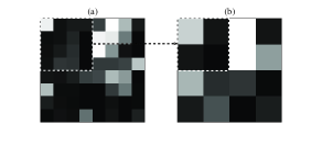
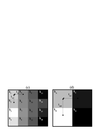
Figure 3.1. A schematic representation of the relation between cell and block permeabilities and transmissibilities. One step in the renormalization algorithm. (a) $8\times 8$ permeability map. (b) The $4\times 4$ coarsened permeability map. Notice how a $4\times 4$ group of cells is substituted by a $2\times 2$ group of blocks. (c) Blow-up of a $2\times 2$ group of cells. (d) Blow-up of a $2\times 2$ group of blocks. Properties of cells are subscripted with numbers, properties of blocks with letters. Permeabilities are indicated by $k$ and transmissibilities with $t$, $k{}_{A}=\left(k_{1}+k_{2}\right)/2,\,t{}_{AB}=\left(t_{23}+t_{67}\right)/2,\,t{}_{AC}=\left(t_{59}+t_{610}\right)/2$.

Accordingly, a renormalization algorithm was implemented whereby groups of $4\times 4$ cells are progressively substituted by groups of $2\times 2$ blocks, until the required degree of coarsening in permeability is achieved. This procedure is fast and can be further improved with the use of parallel computing. Finally, $\mathbf{\mathcal{T}}$ is inverted to obtain the coarse pressure, see Equation (3.10). The procedure in $d$-dimensions is as follows:

1. Start with a permeability map, linear size $N$ multiple of 4. Calculate the pressure by inverting the transmissibility matrix, see Equation (2.2).

2. Subdivide the system into groups of $4^{d}$ cells. Substitute each group with a new group of $2^{d}$ blocks, calculating the new permeability according to the averaging rule, see Appendix and Figure 3.1.

3. The new system has a factor of $2^{d}$ less cells. Calculate the upscaled pressure by inverting the new transmissibility matrix and rescaling, Equation (3.10).

Clearly the higher the dimension, the bigger the advantage in avoiding a double matrix multiplication.

It should be stressed that this renormalization scheme derives directly from the representation of the problem in the mean-field approximation and from the choice of $\mathbf{W}$ matrix. This result relates the elimination of permeability fluctuations to the smoothening of fluctuations in pressure, revealing the basic principle underlying renormalization methods for up-scaling. Importantly, it also represents the starting point for devising a controlled method to include the effects of fluctuations in the coarsening process.

4. Numerical Simulations and Heterogeneities

4.1. Stochastically generated correlated permeability

To emphasize the importance of maintaining the statistical properties of the permeability distribution, various realizations were generated with the same moments. Permeability was simulated as a random, log-normally distributed correlated variable on two- and three-dimensional Cartesian regular grids with a moving average technique Wall:cor .

The starting point is an uncorrelated field, that is normally or uniformly distributed random numbers are assigned to each cell. Then the correlation is introduced by averaging these values with a moving circle technique Wall:cor . By the central limit theorem, the new distribution remains normal, at least for sufficiently big circles, independent of the statistics of the initial data. Moreover, the correlation length is related to the radius of the circle used in the averaging process. Permeability is then taken to be the exponential of this distribution. Anisotropic systems can be generated by using ellipses to account for different rock types in the simulated reservoir.

The upscaled pressure was compared with the simple averaging of the fine pressure. Errors were calculated as differences between the two pressure solutions at the same coarsening level and then averaged over the entire system. While the average error is a useful measure of accuracy, localizing the discrepancies allows us to look for their justification in view of heterogeneities.

4.2. Analysis of heterogeneity in permeability distribution

The simplest test cases to be analysed are two layered systems where exact analytical solutions are known. More precisely, the equivalent permeability for flow parallel to the strata is the arithmetic average of the different permeabilities, and for perpendicular flow it is the harmonic average. In general, these two averages can be shown to be respectively the lower and upper limit on the effective permeability of any system Farmer:krev . As can be expected the new renormalization technique is just as good in these cases as others of its kind. It must be noted that while renormalization according to the resistor analogy produces a final number corresponding to the equivalent permeability, the last step of the wavelet method can only lead to a $2\times 2$ cell. A number can be obtained afterwards, but this is necessarily going to be some kind of average. For example, in the case of vertical layering, while at the third coarsening step the renormalization method already has a homogeneous character, the wavelet method still has a layered structure. The correct result, that is, the harmonic mean, can be recovered by taking the harmonic mean of the two layers. In the case of a chess-board configuration, where resistor analogy renormalization underestimates permeability with an error increasing with the difference between the two layer permeabilities Zimm:ren_comp , the wavelet method overestimates it by an even larger amount. In this case it is possible to show analytically that the exact result should be the geometric mean Farmer:krev while the wavelet method result is the arithmetic mean, as is expected given the averaging which takes place in the algorithm. This is not ideal but at least the error can be predicted and its source clearly identified, see Table 1.

$k_{1}$= 2500, $k_{2}$= 5000	$k_{\textrm{resistor}}$	$k_{\textrm{wavelet}}$	$k_{\textrm{exact}}$
Perpendicular layering	3333	3333	3333
Parallel layering	3750	3750	3750
Chess-board	3429	3750	3535.5

Table 1. Comparison of effective permeability obtained by resistor and wavelet based renormalization for layered and chess-board systems with cells of low ($k_{1}$) and high ($k_{2}$) homogeneous permeability reduced to a single cell. Both methods predict the exact results correctly for the layered cases while both fail in the chess-board case.

Initially two-dimensional systems were analysed so the method described will refer to this case. Results are also presented in three dimensions, where the procedure is identical in concept.

First, an analysis was made on the permeability distribution at each up-scaling step, see Table 2.

Cell size	Mean	Std
1	4902.9	11.8597
2	4902.8	11.54
4	4902.9	11.05
8	4903.1	10.24
16	4903.9	8.36

Table 2. Statistics of permeability distribution at each coarsening step, for a $64\times 64$ system, with correlation length $r=10$ averaged over 10 realizations. At each up-scaling step the cell size doubles. Notice how the renormalization preserves the mean and how the standard deviation starts to decrease considerably only when the cell size is comparable to the correlation length.

Once the permeability maps had been generated, pressure boundary conditions were set on the left and right boundaries of the system. These were taken to be fixed at 100 on the left and 50 on the right. The drop in pressure across the system is a fundamental factor in determining the errors in the estimates. However, the use of relative errors mitigates this effect and the same boundary conditions were used in all the simulations. A pressure profile was obtained at each renormalization step inverting the corresponding transmissibility matrix with the correct renormalized boundary conditions and compared to an equally coarsened pressure obtained by successively averaging fine pressure on $2\times 2$ cells, see Figure 4.1. The process was repeated $10$ times to generate a distribution of results.

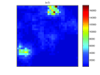
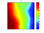
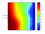
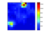
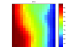
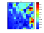
Figure 4.1. Wavelet renormalization of a permeability map from $32\times 32$ to $16\times 16$. (a1) Fine scale permeability. (a2) Fine scale pressure solution obtained from fine scale permeability. (a3) Average of the fine scale pressure solution ($2\times 2$ cells averaged). (b1) Wavelet renormalized coarse permeability. (b2) Coarse pressure solution obtained from coarse permeability. (b3) Modulus of relative error, $\left|\textrm{a3-b2}\right|$/a3. In this case the relative difference between the averaged fine scale pressure (a3) and the coarse pressure (b2) is within 2%. This procedure was repeated for systems with varying permeability ranges and with different heterogeneities, simulating different rock types.

When averaged over many realizations, the absolute error between the averaged fine scale pressure and the coarse pressure obtained from the wavelet upscale was consistently found to be of order $10^{-3}$. For this kind of systems, errors in a single realizations did not exceed 5%.

As expected, the error was found to be higher with higher standard deviation of the permeability, see Table 3, but only for very heterogeneous systems, where the standard deviation is an order of magnitude larger than the mean.

$\sigma/\mu$	Mean relative error (10-3)	Std of error (10-3)
0.1	$-$5.23	3.41
0.2	$-$0.74	3.47
0.4	$-$0.84	3.34
0.8	$-$1.46	3.15
1	0.58	3.64
2	1.82	3.52
10	0.79	4.71

Table 3. Comparison of mean and standard deviation of the relative error at different standard deviation of permeability and same correlation length $r$=3, $\mu$=10000, averaged over entire system. All data averaged over 27 realizations of $32\times 32$ systems being upscaled to $16\times 16$.

Correlation length	Mean relative error (10-3)	Std of error (10-3)
1	$-$0.52	3.85
2	$-$0.49	3.51
3	0.67	3.46
4	0.64	3.45
5	0.66	3.43

Table 4. Comparison of error for different correlation lengths but same standard deviation, $\sigma$=1000, $\mu=1000$ (average of multiple realizations of $32\times 32$ systems being upscaled to $16\times 16$, see text for details about the number of realizations). Notice a very weak dependence of the standard deviation of the error on the correlation length that seems to suggest that a more correlated system can be upscaled more accurately.

Next, a comparison between realizations with varying correlation length $r$, expressed in terms of grid cells, and equal standard deviation in permeability was made. A different number of realizations were averaged depending on the correlation length of the system, considering that each subsystem of linear size equal to the correlation length constitutes a sample in statistical terms (number of realizations = $3r^{2}$). As can be seen in Table 4, the more the field is correlated, that is, the larger the value of $r$, the better the wavelet renormalization method approximates the fine scale pressure average. However, even at a radius of correlation equal to one grid cell, the average standard deviation of the error is within 0.4%.

While the error averaged over the entire system can be misleadingly small, due to cancellations which occur between positively and negatively biased results at specific locations, the standard deviation of the error over the system can be taken as a faithful indicator of the performance of the method.

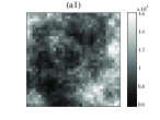
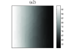
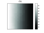
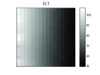
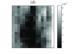
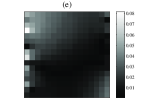
Figure 4.2. Comparison of resistor and wavelet renormalization. (a1) Fine scale permeability. (a2) Fine scale pressure solution obtained from fine scale permeability. (b) Coarse pressure solution obtained with wavelet method. (c) Coarse pressure solution obtained with resistor method. (d) Modulus of relative error of pressure obtained with the wavelet method with respect to the pressure average. (e) Modulus of relative error of pressure obtained with the resistor method with respect to the pressure average. The error in the wavelet renormalization is of order $10^{-3}$ because the permeability field is fairly homogeneous. However, the resistor renormalization is less effective even in this ideal case.

A comparison with the resistor renormalization performed according to King:immis (equation 2.1), can be seen in Figure (4.2). It is possible to develop a more accurate resistor renormalization algorithm by considering the anisotropy generated by the upscaling process. However, this algorithm is not as immediate as the wavelet renormalization algorithm to implement, requiring the definition of two transmissibilities per cell. It must be noted that, while the wavelet method is geared towards reproducing the average pressure, the resistor method is based on flux conservation, thus it is not surprising that the results of the two methods differ.

4.3. Shales

One of the major drawbacks of the renormalization proposed by King:renkeff is its imprecise treatment of shales. When the permeability contrast between adjacent cells is high, for example at the interface between permeable rock such as sandstone, and impermeable elements such as shales, the analogy with resistors gives inaccurate predictions. This results in a deformation of shales which can lead to misjudgment of the reservoir connectivity. Typically, shales have a large aspect ratio and they are distributed horizontally often constituting a barrier to flow in the vertical direction. A successful alternative approach to shales is given in Ref. Begg:vertsh , where the permeability is related to the length of the path going around the shale bodies.

Shales were implemented in the following way: some of the sites of the system were chosen at random and shales of random size and aspect ratio were created by setting the permeabilities in the area to a very small value ($10^{-13}$). Another conventional way of implementing shales into a model is to make correlation very anisotropic. This causes areas of low permeability to naturally emerge with the correct aspect ratio and orientation. However, the chosen method provides a much greater difference between the low permeability of the shales and the distribution of the permeability in the sand, which is often characteristic of physical systems.

As can be seen in Figure 4.3 and Table 5, shales are correctly upscaled unless their size becomes comparable to the size of the cells.

Max width	Max height	Shale fraction (%)	Mean error(10-3)	Std of error(10-3)
2	2	3.2	18.29	16.2
2	2	33.4	113.85	100.8
16	5	16.4	9.1	25.3
16	5	33.4	6.73	27.1
16	5	57.6	3.1	24.9
5	16	18.8	48.7	46
5	16	36	26.8	47.9
5	16	52.2	20.3	60

Table 5. Error in up-scaling a system with shales with different aspect ratio. Shale permeability set to $10^{-13}$ . All values were averaged over 3 runs. Notice that vertical and small shales are associated with a bigger error.

When either the shale fraction or the sand fraction approaches the percolation threshold, the error of the wavelet method calculated with respect to the average of the fine pressure solution can be of order $10^{-1}$. In this case shales will either cover the entire system or tend to disappear. Anisotropy also plays an important role. Shales perpendicular to the flow seem to represent more of a problem, since they oppose the pressure gradient, see Table 5, bottom three entries. For example, in Figure 4.3, the largest error occurs in the lower central region where a vertical barrier disappears in the coarsening process. However, in this situation, it is debatable that averaging the pressure profile can be of any use. Visually, it is clear that the upscaled pressure profile reproduces the fine scale pressure profile with reasonable accuracy. The resistor renormalization, as defined in Section 4.2, produces very unsatisfactory results. It must be noted that, even at the fine scale, pressure in very nearly zero permeability areas is poorly defined.

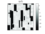
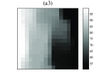
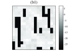
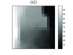
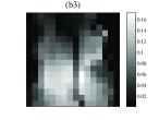
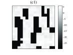
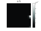
Figure 4.3. Wavelet transform based real-space renormalization of a permeability map with vertical shales from $32\times 32$ to $16\times 16$. (a1) Fine scale permeability. (a2) Fine scale pressure solution obtained from fine scale permeability. (a3) Average of the fine scale pressure solution ($2\times 2$ cells averaged). (b1) Wavelet-renormalized coarse permeability. (b2) Coarse pressure solution obtained from b1. (b3) Modulus of relative error, $\left|\textrm{a3-b2}\right|$/a3. (c1) Resistor-renormalized coarse permeability. (c2) Coarse pressure solution obtained from c1. (c3) Modulus of relative error, $\left|\textrm{c3-c2}\right|$/c3. The relative difference between the averaged fine scale pressure and the coarse pressure from wavelet renormalization reaches 16% with an average of 6%. Resistor renormalization clearly doesn’t produce the required result. The shale permeability is set to $10^{-13}$and also the shales are distributed across the direction of flow, generating a worst case scenario.

4.4. Three-dimensional systems

As already mentioned, the wavelet renormalization method for up-scaling is easily extended to three-dimensional systems. In this case, no flow was assumed in two directions and pressures were specified on the boundaries of the third direction. The only difference in the procedure between two- and three-dimensional systems is the structure and size of the matrix $\mathbf{W}$. As for the two-dimensional case, by observing the structure of the transformed transmissibility matrix $\mathcal{T}$, a renormalization scheme can be devised to produce the coarse permeability avoiding the matrix multiplications. The algorithm substitutes cubes of linear size 4 cells by cubes of half the linear size. Preliminary runs confirm that the upscale procedure is approximately as accurate as it is in the two-dimensional case.

5. Conclusion

An up-scaling method, based on the Haar wavelet transform and real-space renormalization was presented. Its advantages are speed, due to the underlying renormalization algorithm, and a rigorous mathematical derivation of the up-scaling rule.

This algorithm emerges from a mean-field picture of the solution to Darcy’s equation, which is at the heart of the success of renormalization methods. The renormalization scheme is a consequence of the choice of $\mathbf{W}$ matrix, in this case the aim is to obtain the coarse permeability map that would generate the average pressure profile. A different matrix would lead to mathematically valid results, for example one where the block permeability is taken to be equal to the value at the top left cell in the group constituting the block. However, the present choice attempts to minimize the information loss inherent in the coarsening process while preserving the algorithm simplicity to ensure its efficiency.

Within this context, the lowest degree, mean-field approximation, in which all fluctuations are neglected, performs well in two and three dimensions. The main problems with this method are encountered when there is a high contrast in permeability, such as in the case of shales, which leads to sharp pressure changes that inevitably get smoothened out. The resistor renormalization fails even more drastically in this case. A different wavelet matrix choice would improve the performance of the method. It is nevertheless foreseeable that the emerging renormalization scheme would not be as easy to implement as the one presented. An exact solution could also be obtained, including all the fluctuation terms, however, the computational power required would be equivalent to performing the fine-scale solution.

At present, the method can be used as a fast upscaling technique able to cope with heterogeneities. The formalism introduced highlights how a very crude renormalization scheme is satisfactory in treating sufficiently homogeneous systems and how upscaling methods can be constructed to match the specifications of the problem and the required results. The resistor method is based on an analogy with current laws and is therefore a statement of conservation of flux. It is possible that by defining Darcy’s equation in terms of fluxes rather than permeability and pressure, one might be able to find a matrix analogy to the resistor method that will reproduce the resistor upscaling rule in the same way as the current $\mathbf{W}$ matrix produces the renormalization scheme that was proposed. The present framework can be applied to other problems, such as advective transport, leading to insights into the general issue of how operators change as a consequence of coarsening.

It is hoped that further study will shed light on the effect of adding fluctuations to the mean-field approximation, allowing the choice between different degrees of accuracy depending on the available computational time.

6. Acknowledgements

V.P. gratefully acknowledges funding from the Department of Earth Science and Engineering, Imperial College London and the authors are thankful to the anonymous referees for very useful comments.

7. Appendix

In the following we reproduce the structure of the matrices discussed in the text. The structure of the transmissibility matrix for a $4\times 4$ system:

$\mathbf{T}=\left[\begin{array}[]{cccccccc}2k_{1}+t_{1,2}+t_{1,5}&-t_{1,2}&0&0&-t_{1,5}&0&...&0\\ -t_{2,1}&2k_{2}+t_{2,3}+t_{2,5}&-t_{2,3}&0&0&-t_{2,5}&...&0\\ ...&...&...&...&...&...&...&-t_{15,16}\\ 0&0&0&0&0&.&-t_{16,15}&2k_{16}+t_{16,15}+t_{16,12}\end{array}\right]$

The upper corner of the transformed matrix: $\mathbf{\mathcal{T}}=\mathbf{WTW^{T}}$

$$\mathbf{\mathcal{T}}=\left[\begin{array}[]{cccc}k_{1}+k_{2}+\frac{t_{23}+t_{67}}{2}+\frac{t_{59}+t_{610}}{2}&-\frac{t_{23}+t_{67}}{2}&-\frac{t_{59}+t_{610}}{2}&0\\ -\frac{t_{23}+t_{67}}{2}&k_{3}+k_{4}+\frac{t_{23}+t_{67}}{2}+\frac{t_{711}+t_{812}}{2}&0&-\frac{t_{711}+t_{812}}{2}\\ -\frac{t_{59}+t_{610}}{2}&0&k_{13}+k_{14}+\frac{t_{59}+t_{610}}{2}+\frac{t_{1011}+t_{1415}}{2}&-\frac{t_{1011}+t_{1415}}{2}\\ 0&-\frac{t_{711}+t_{812}}{2}&-\frac{t_{1011}+t_{1415}}{2}&k_{15}+k_{16}+\frac{t_{711}+t_{812}}{2}+\frac{t_{1011}+t_{1415}}{2}\end{array}\right]$$

The transmissibility matrix for a $2\times 2$ system, the dash indicates that the properties refer to the $2\times 2$ system :

$$\mathbf{T^{\prime}}=\left[\begin{array}[]{cccc}2k^{\prime}_{1}+t^{\prime}_{1,2}+t^{\prime}_{1,3}&-t^{\prime}_{1,2}&-t^{\prime}_{1,3}&0\\ -t^{\prime}_{2,1}&2t^{\prime}_{2}+t^{\prime}_{2,1}+t^{\prime}_{2,4}&0&-t^{\prime}_{2,4}\\ -t^{\prime}_{1,3}&0&2t^{\prime}_{3}+t^{\prime}_{3,1}+t^{\prime}_{3,4}&-t^{\prime}_{3,4}\\ 0&-t^{\prime}_{2,4}&-t^{\prime}_{3,4}&2k^{\prime}_{4}+t^{\prime}_{2,4}+t^{\prime}_{3,4}\end{array}\right]$$

Relationship between permeability and transmissibility in the upscaled system ($k^{\prime}_{i}$, $t^{\prime}_{ij}$) and in the fine scale system ($k{}_{i}$, $t{}_{ij}$):

$$k^{\prime}_{1}=\frac{k_{1}+k_{2}}{2},\,\,\,\,t^{\prime}_{12}=\frac{t_{23}+t_{67}}{2},\,\,\,\,t^{\prime}_{13}=\frac{t_{59}+t_{610}}{2}\,\,\,\,\textrm{etc}.$$

References

- [1] A. Aldroubi and M. Unser, Wavelets in medicine and biology, CRC Press, 1996.
- [2] K. Aziz and A. Settari, Petroleum reservoir simulation, Kluwer Academic Publishers, 1979.
- [3] S.H. Begg and P.R. King, Modelling the effect of shales in reservoir performance: calculation of vertical effective permeability, Presented at the SPE Reservoir Simulation Symposium, Dallas, TX, Feb. 10-13, SPE Paper 13529, 1985.
- [4] C. Best, Wavelet induced renormalization group for the landau-ginzburg model, Nuclear Physics B, (Proc. Suppl.) 83-84 (2000), 848–850.
- [5] I. Daubechies, Ten lectures on wavelets, CBMS-NSF Regional conference series in applied mathematics, SIAM, Philadelphia, 1992.
- [6] L.J. Durlofsky, Upscaling and gridding of fine scale geological models for flow simulation, Paper presented at the 8th International Forum on Reservoir Simulation, Iles Borromees, Stresa, Italy, June 20-24, 2005.
- [7] F. Ebrahimi and M. Sahimi, Multiresolution wavelet scale up of unstable miscible displacements in flow through heterogeneous porous media, Transport in Porous Media 57 (2004), 75–102.
- [8] C.L. Farmer, Upscaling: a review, Int. J. for Num. Meth. in Fluids 40(1-2) (2002), 63–78.
- [9] A. Haar, Zur thaeorie der orthogonalen funktionensysteme, Ph.D. thesis, Goettingen, 1909.
- [10] J.J. Hastings and A.H. Muggeridge, Upscaling uncertain permeability using small cell renormalization, Mathematical geology 33 (2001), 491.
- [11] D.T. Hristopulos, Renormalization group methods in subsurface hydrology: overview and applications in hydraulic conductivity upscaling, Advances in Water Resources 26(12) (2003), 1279–1308.
- [12] D.T. Hristopulos and G. Christakos, Renormalization group analysis of permeability upscaling, Stochastic Environmental Research and Risk Assessment 13(12) (1999), 131–160.
- [13] A.E. Ismail, G.C. Rutledge, and G. Stephanopoulos, Multiresolution analysis in statistical mechanics, part i. using wavelets to calculate thermodynamic properties, J. Chem. Phys. 118 (2003), no. 10, 4414–4423.
- [14] by same author, Using wavelet transforms for multiresolution materials modeling, Computers and Chemical Engineering 29 (2005), 689.
- [15] L.P Kadanoff, Scaling laws for ising models near tc, Physica 2 (1966), 263–272.
- [16] P. R. King, The use of renormalization for calculating effective permeability, Transport in Porous Media 4 (1989), 37–58.
- [17] by same author, Upscaling permeability: Error analysis for renormalization, Transport in Porous Media 23 (1996), 337–354.
- [18] P. R. King, A.H. Muggeridge, and W.G Price, Renormalization calculations of immiscible flow, Transport in Porous Media 12 (1993), 237–260.
- [19] J. L. Larsonneur and J. Morlet, Wavelets and Seismic Interpretation, Wavelets. Time-Frequency Methods and Phase Space, 1989.
- [20] B. Noetinger, V. Artus, and G. Zargar, The future of stochastic and upscaling methods in hydrogeology, Hydrogeology Journal 13(1) (2005), 184–201.
- [21] A.E. O’Sullivan and M.A. Christie, Solution error models: a new approach for coarse grid history matching, 2005, Presented at the SPE Reservoir Simulation Symposium, Houston, TX, Jan. 31 - Feb. 2, SPE Paper 93268.
- [22] T.C. Wallstrom, S.L. Hou, M.A. Christie, L.J. Durlofsky, and D.H. Sharp, Accurate scale up of two phase flow using renormalization and nonuniform coarsening, Computational Geoscience 3 (1999), 69–87.
- [23] X.H. Wen and J.J. Gomez-Hernandez, Upscaling hydraulic conductivities in heterogeneous media: An overview, Journal of Hydrology 183 (1996), ix–xxxii.
- [24] J.K. Williams, Simple renormalization schemes for calculating effective properties of heterogeneous reservoirs, Mathematics of oil recovery (P.R. King, ed.), Clarendon Press, Oxford, 1992, p. 281.
- [25] I. Yeo and R.W. Zimmerman, Accuracy of the renormalization method for computing effective conductivities of heterogeneous media, Transport in Porous Media 45 (2001), 129–138.