An ab-initio theory for the temperature dependence of magnetic anisotropy

Abstract

We present a first-principles theory of the variation of magnetic anisotropy, $K$, with temperature, $T$, in metallic ferromagnets. It is based on relativistic electronic structure theory and calculation of magnetic torque. Thermally induced ‘local moment’ magnetic fluctuations are described within the relativistic generalisation of the ‘disordered local moment’ (R-DLM) theory from which the $T$ dependence of the magnetisation, $m$, is found. We apply the theory to a uniaxial magnetic material with tetragonal crystal symmetry,$L1_{0}$-ordered FePd, and find its uniaxial $K$ consistent with a magnetic easy axis perpendicular to the Fe/Pd layers for all $m$ and proportional to $m^{2}$ for a broad range of values of $m$. This is the same trend that we have previously found in $L1_{0}$-ordered FePt and which agrees with experiment. This account, however, differs qualitatively from that extracted from a single ion anisotropy model. We also study the magnetically soft cubic magnet, the $Fe_{50}Pt_{50}$ solid solution, and find that its small magnetic anisotropy constant $K_{1}$ rapidly diminishes from 8 $\mu$eV to zero. $K$ evolves from being proportional to $m^{7}$ at low $T$ to $m^{4}$ near the Curie temperature.

I INTRODUCTION

It is well-known that a description of magnetic anisotropy, K, can be provided once relativistic effects such as the spin-orbit coupling on the electronic structure of materials are considered. Over recent years ‘first-principles’ theoretical work, based on relativistic density functional theory, has been quite successful in describing trends in K for a range of magnetic materials in bulk, film and nanostructured form Jansen ; Kubler ; review , e.g. Razee+99 ; Shick ; Till ; Laz ; Qian ; Cabria . These results can be fed into micromagnetic models of the magnetic properties to describe phenomena such as magnetisation reversal processes in magnetic recording materials micromag . There are also implications for electronic transport effects such as anisotropic magnetoresistance (AMR) AMR . Until only very recently, however, the temperature dependence of K was assumed to follow that given by single ion anisotropy models developed by Callen and Callen and others over 40 years ago Callen This assumption has now been challenged by ab-initio electronic structure theory Mryasov ; MAEvsT . The unexpected dependence of the magnetic anisotropy of $L1_{0}$-FePt, found in experiment Okamoto ; Thiele2002 ; Wu , to decrease in proportion with the square of the magnetisation, $m(T)$, is described well by the new theoretical treatments whereas the single ion magnetic anisotropy models fail. Evidently the itinerant nature of the electrons in metallic magnets like $FePt$ is an important factor.

In this paper we present a detailed description of our ab-initio theory for the temperature dependence of magnetic anisotropy. It involves a fully relativistic description of the electronic structure and hence includes spin-orbit coupling effects. The thermally excited magnetic fluctuations are accounted for with the, by now, well-tried, disordered local moment (DLM) picture. Moriya ; DLM ; JBS+BLG

The study of temperature-dependent magnetic anisotropy has recently become particularly topical owing to extensive experimental studies of magnetic films and nanostructures and their technological potential. For example, fabrication of assemblies of increasingly smaller magnetic nanoparticles has great potential in the design of ultra-high density magnetic data storage media. Sun If thermally driven demagnetisation and loss of data is to be avoided over a reasonable storage period, there is, however, a particle size limit to confront. A way of reducing this limit is to use materials with high magnetocrystalline anisotropy, $K$, since the superparamagnetic diameter of a magnetic particle is proportional to $(k_{B}T/K)^{\frac{1}{3}}$, where $k_{B}T$ is the thermal energy. OHandley Writing to media of very high $K$ material can be achieved by temporary heating. Thiele2002 ; TAR $K$ is reduced significantly during the magnetic write process and the information is locked in as the material cools. Modelling this process and improving the design of high density magnetic recording media therefore requires an understanding of how $K$ varies with temperature.

The temperature dependence of magnetic anisotropy in magnets where the magnetic moments are well-localised, e.g. rare-earth and oxide magnets, is described rather well by these single ion anisotropy models but it is questionable whether this will also be the case for itinerant ferromagnets. OHandley Owing to its high uniaxial magnetocrystalline anisotropy (MCA) (4-10 10⁷ ergs/cm³ or up to 1.76 meV per $FePt$ pair FePt-MAE ; Farrow ) the chemically ordered $L1_{0}$ phase of equiatomic $FePt$, has attracted much attention as a potential ultra-high magnetic recording density material. Indeed arrays of $FePt$ nanoparticles with diameters as small as 3 nm have been synthesised. Sun ; Wu For a uniaxial magnet like this, $K$ is the difference between the free energies, $F^{(0,0,1)}$ and $F^{(1,0,0)}$ of the system magnetised along $(0,0,1)$ and $(1,0,0)$ crystallographic directions. So for the first application of our theory we chose $L1_{0}$-ordered $FePt$. MAEvsT Careful experimental studies of its fundamental magnetic properties. Okamoto ; Thiele2002 ; Wu find that over a large temperature range, $K(T)/K(0)=(m(T)/m(0))^{n}$ ,where $n=2$ instead of $n=3$ as expected from the simple single ion anisotropy model. We found our ab-initio calculations to be in good agreement with this surprising result. Mryasov et al. Mryasov independently examined the same issues with a different theoretical but complementary approach and drew the same conclusions. In this paper, after providing full details of the R-DLM theory of magnetic anisotropy, we explore whether this $(m(T)/m(0))^{2}$ behavior is a general property of the MCA of $L1_{0}$-ordered itinerant transition metal uniaxial magnets by investigating another important uniaxial magnetic material $FePd$. We also study the temperature dependence of a material which has cubic rather than the tetragonal crystal symmetry of $L1_{0}$-ordered alloys, and which is magnetically softer, namely compositionally disordered $FePt$.

In the next section we describe the temperature dependence of the magnetic anisotropy that emerges from classical spin models with single site anisotropy. We then review briefly current approaches to calculating $K$ from first-principles electronic theory of materials at $T=0$K. An outline of the ‘disordered local moment’ (DLM) picture of metallic magnetism at finite temperature precedes a description of its relativistic generalisation. It is shown how the temperature dependence of the magnetisation, $m(T)$, can be found. The key outcome from the R-DLM theory is the formalism for the magnetisation dependence of magnetic anisotropy ab-initio. Applications to uniaxial $L1_{0}$-FePd and cubic $Fe_{50}Pt_{50}$ follow and the final section provides a summary.

II SINGLE ION ANISOTROPY

The MCA of a material can be conveniently expressed as $K=\sum_{\gamma}K_{\gamma}g_{\gamma}(\hat{n})$ where the $K_{\gamma}$’s are coefficients, $\hat{n}$ is the magnetisation direction and $g_{\gamma}$’s are polynomials (spherical harmonics) of the angles $\vartheta$, $\varphi$, fixing the orientation of $\hat{n}$ with respect to the crystal axes, and belong to the fully symmetric representation of the crystal point group. As the temperature rises, $K$ decreases rapidly. The key features of the results of the early theoretical work on this effect Callen are revealed by classical spin models pertinent to magnets with localised magnetic moments. The anisotropic behavior of a set of localised ‘spins’ associated with ions sitting on crystalline sites, $i$, in the material, is given by a term in the hamiltonian $H_{an}=\sum_{i}\sum_{\gamma}k_{\gamma}g_{\gamma}(\widehat{e}_{i})$ with $\widehat{e}_{i}$ a unit vector denoting the spin direction on the site $i$. As the temperature is raised, the ‘spins’ sample the energy surface over a small angular range about the magnetisation direction and the anisotropy energy is given from the difference between averages taken for the magnetisation along the easy and hard directions. If the coefficients $k_{\gamma}$ are assumed to be rather insensitive to temperature, the dominant thermal variation of $K$ for a ferromagnet is given by $K(T)/K(0)=\langle g_{l}(\widehat{e})\rangle_{T}/\langle g_{l}(\widehat{e})\rangle_{0}$ The averages $\langle\cdots\rangle_{T}$ are taken such that $\langle\widehat{e}\rangle_{T}=m(T)$, the magnetisation of the system at temperature $T$, and $l$ is the order of the spherical harmonic describing the angular dependence of the local anisotropy i.e. $l=2$ and $4$ for uniaxial and cubic systems respectively. At low temperatures $K(T)/K(0)\approx(m(T)/m(0))^{l(l+1)/2}$ and near the Curie temperature $T_{c}$, $K(T)/K(0)\approx(m(T)/m(0))^{l}$.

These results can be illustrated straightforwardly in a way which will be helpful for the development of our ab-initio theory. Consider a classical spin hamiltonian appropriate to a uniaxial ferromagnet.

$$H=-\frac{1}{2}\sum_{i,j}J_{ij}\widehat{e}_{i}\cdot\widehat{e}_{j}-k\sum_{i}(\widehat{n}_{0}\cdot\widehat{e}_{i})^{2}$$ (1)

where $\widehat{e}_{i}$ describes the orientation of a classical spin at site $i$ and $J_{ij}$ and $k$ are exchange and anisotropy parameters. $\widehat{n}_{0}$ is a unit vector along the magnetic easy axis. A mean field description of the system is given by reference to a hamiltonian $\sum_{i}\vec{h}\cdot\widehat{e}_{i}$ where the orientation of Weiss field $\vec{h}$, i.e. $\vec{h}=h\widehat{n}$, determines the direction of the magnetisation of the system and has direction cosines ($\sin\vartheta\cos\varphi$, $\sin\vartheta\sin\varphi$, $\cos\vartheta$). Within this mean field approximation the magnetisation $m$ is $\vec{m}(T)=\int\widehat{e}\;P(\widehat{e})d\widehat{e}$ where the probability of a spin being orientated along $\widehat{e}$ is $P(\widehat{e})=e^{-\beta h\widehat{n}\cdot\widehat{e}}/Z_{0}$ with $Z_{0}=\int e^{-\beta h\widehat{n}\cdot\widehat{e}}d\widehat{e}$. The free energy difference per site between the system magnetised along two directions $\widehat{n}_{1}$ and $\widehat{n}_{2}$ is

$$K(T)=-\frac{k}{Z_{0}}\int((\widehat{n}_{0}\cdot\widehat{e})^{2}e^{-\beta h\widehat{n}_{1}\cdot\widehat{e}}-(\widehat{n}_{0}\cdot\widehat{e})^{2}e^{-\beta h\widehat{n}_{2}\cdot\widehat{e}})d\widehat{e}$$ (2)

If $\widehat{n}_{1}$ and $\widehat{n}_{2}$ are parallel and perpendicular to the magnetic easy axis $\widehat{n}_{0}$ respectively then

$$K(T)=-\frac{k}{Z_{0}}\int g_{2}(\widehat{n}_{0}\cdot\widehat{e})e^{-\beta h\widehat{n}_{0}\cdot\widehat{e}}d\widehat{e}$$ (3)

where $g_{2}$ is the Legendre polynomial $(3(\widehat{n}_{0}\cdot\widehat{e})^{2}-1)/2$. As a function of the magnetisation $m(T)/m(0)$, $K(T)/K(0)$ varies quadratically near the Curie temperature $T_{c}$ and cubically at low $T$. The same dependence can be shown for this simple spin model for the rate of variation of magnetic anisotropy with angle $\vartheta$ that the magnetisation makes with the system’s easy axis, namely the magnetic torque OHandley $T_{\vartheta}=-\partial K/\partial\vartheta$.

III AB-INITIO THEORY OF MAGNETIC ANISOTROPY

Magnetocrystalline anisotropy is caused largely by spin-orbit coupling and receives an ab-initio description from the relativistic generalisation of spin density functional (SDF) theory. Jansen Apart from the work by Mryasov et al. Mryasov and ourselves MAEvsT , up to now calculations of the anisotropy constants $K$ have been suited to $T=0$K only. Spin-orbit coupling effects are treated perturbatively or with a fully relativistic theory Razee+97 ; Razee+99 . Typically the total energy, or the single-electron contribution to it (if the force theorem is used), is calculated for two or more magnetisation directions, $\hat{n}_{1}$ and $\hat{n}_{2}$ separately and then the MCA is obtained from the difference, $\Delta E$. $\Delta E$ is typically small ranging from meV to $\mu$eV and high precision in calculating the energies is required. For example, we have used this rationale with a fully relativistic theory to study the MCA of magnetically soft, compositionally disordered binary and ternary component alloys Razee+97 ; more and the effect upon it of short-range Razee+99 and long range chemical order ICNDR in harder magnets such as $CoPt$ and $FePt$.

Experimentally, measurements of magnetocrystalline anisotropy constants of magnets can be obtained from torque magnetometry OHandley . From similar considerations of magnetic torque, ab-initio calculations of MCA can be made. There are obvious advantages in that the MCA can be obtained from a single calculation and reliance is not placed on the accurate extraction of a small difference between two energies. In particular the torque method has been used to good effect by Freeman and co-workers Wang-torque in conjunction with their state-tracking method to study the MCA of a range of uniaxial magnets including layered systems.

If the free energy of a material magnetised along a direction specified by $\widehat{n}=$ ( $\sin\vartheta\cos\varphi$, $\sin\vartheta\sin\varphi$, $\cos\vartheta$ ) is $F^{(\widehat{n})}$, then the torque is

$$\vec{T}^{(\widehat{n})}=-\frac{\partial F^{(\widehat{n})}}{\partial\widehat{n}}.$$ (4)

The contribution to the torque from the anisotropic part of $F^{(\widehat{n})}$ leads to a direct link between the gap in the spin wave spectrum and the MCA by the solution of the equation Russian-spinwave

$$\frac{d\widehat{n}}{dt}=\gamma(\widehat{n}\wedge\vec{T}^{(\widehat{n})}).$$ (5)

where $\gamma$ is the gyromagnetic ratio. Closely related to $\vec{T}^{(\widehat{n})}$ is the variation of $F^{(\widehat{n})}$ with respect to $\vartheta$ and $\varphi$, i.e. $T_{\vartheta}(\vartheta,\varphi)=-\frac{\partial F^{(\widehat{n})}}{\partial\vartheta}$ and $T_{\varphi}(\vartheta,\varphi)=-\frac{\partial F^{(\widehat{n})}}{\partial\varphi}$. As shown by Wang et al. Wang-torque , for most uniaxial magnets, which are well approximated by a free energy of the form

$$F^{(\widehat{n})}=F_{iso}+K_{2}\sin^{2}\vartheta+K_{4}\sin^{4}\vartheta,$$ (6)

(where $K_{2}$ and $K_{4}$ and magnetocrystalline anisotropy constants and $F_{iso}$ is the isotropic part of the free energy), $T_{\vartheta}(\vartheta=\pi/4,\varphi=0)=-(K_{2}+K_{4})$. This is equal to the MCA, $\Delta F=F^{(1,0,0)}-F^{(0,0,1)}$. For a magnet with cubic symmetry so that

$$F^{(\widehat{n})}\approx F_{iso}+K_{1}(\sin^{4}\vartheta\sin^{2}2\varphi+\sin^{2}2\vartheta),$$ (7)

a calculation of $T_{\varphi}(\vartheta=\pi/2,\varphi=\pi/8)$ gives $-K_{1}/2$. In this work we present our formalism for the direct calculation of the torque quantities $T_{\vartheta}(\vartheta,\varphi)$ and $T_{\varphi}(\vartheta,\varphi)$, and hence the MCA, in which the effects of thermally induced magnetic fluctuations are included so that the temperature dependence is captured.

In our formalism the motion of the electron is described with spin-polarised, relativistic multiple scattering theory. An adaptive mesh algorithm EB+BG for Brillouin zone integrations is used in the calculations to ensure adequate numerical precision for the MCA to within 0.1 $\mu$eV Razee+97 ; Razee+99 . Since we characterise the thermally induced magnetic fluctuations in terms of disordered local moments, we now go on to describe this picture of finite temperature magnetism.

IV METALLIC MAGNETISM AT FINITE TEMPERATURES - ‘DISORDERED LOCAL MOMENTS

In a metallic ferromagnet at $T=0$K the electronic band structure is spin-polarised. With increasing temperature, spin fluctuations are induced which eventually destroy the long-range magnetic order and hence the overall spin polarization of the system’s electronic structure. These collective electron modes interact as the temperature is raised and are dependent upon and affect the underlying electronic structure. For many materials the magnetic excitations can be modelled by associating local spin-polarisation axes with all lattice sites and the orientations $\{\hat{e}\}$ vary very slowly on the time-scale of the electronic motions. Moriya These ‘local moment’ degrees of freedom produce local magnetic fields on the lattice sites which affect the electronic motions and are self-consistently maintained by them. By taking appropriate ensemble averages over the orientational configurations, the system’s magnetic properties can be determined.

This ‘disordered local moment’ (DLM) picture has been implemented within a multiple-scattering (Korringa-Kohn-Rostoker, KKR) KKR ; KKR-CPA ; scf-kkr-cpa formalism using the first-principles approach to the problem of itinerant electron magnetism. At no stage does it map the many-electron problem onto an effective Heisenberg model, and yet it deals, quantitatively, with both the ground state and the demise of magnetic long-range order at the Curie temperature in a material-specific, parameter-free manner. It has been used to describe the experimentally observed local exchange splitting and magnetic short-range order in both ultra-thin Fe films fccFe-2002 and bulk Fe, the damped RKKY-like magnetic interactions in the compositionally disordered CuMn ’spin-glass’ alloys MFL-EPL and the quantitative description of the onset of magnetic order in a range of alloys DLM-alloys ; invar-Entel . In combination with the local self-interaction correction (L-SIC) LSIC for strong electron correlation effects, it also gives a revealing account of magnetic ordering in rare earths Ian-Gd . Other applications of the DLM picture include dilute magnetic semiconductors Dederichs and actinides sweden . Short-range order of the local moments can be explicitly included by making use of the recently developed KKR- nonlocal-CPA (KKR-NLCPA) Rowlands ; NLCPA-totE .

We now briefly recap on how this ‘disordered local moment’ (DLM) picture is implemented using the KKR-CPA and how a ferromagnetic metal both above and below the Curie temperature can be described. Our main objective in this paper is to explain its relativistic extension and show how this leads to an ab-initio theory of the temperature dependence of magnetic anisotropy when relativistic effects are explicitly included.

V RELATIVISTIC DISORDERED LOCAL MOMENT THEORY

V.1
General framework

The non-relativistic version of the DLM theory has been discussed in detail by Gyorffy et al. DLM ; JBS+BLG Here we summarise the general framework and concentrate on those aspects which are necessary for a description of magnetic anisotropy. The starting point is the specification of $\Omega^{(\widehat{n})}(\{\widehat{e}\})$, the ‘generalised’ electronic grand potential taken from the relativistic extension of spin density functional theory (SDFT) DLM ; Jansen . It specifies an itinerant electron system constrained such that the local spin polarisation axes are configured according to $\{\widehat{e}\}=\{\widehat{e}_{1},\widehat{e}_{2},\ldots,\widehat{e}_{N}\}$ where $N$ is the number of sites (moments) in the system. For magnetic anisotropy to be described, relativistic effects such as spin-orbit coupling upon the motion of the electrons must be included. This means that orientations of the local moments with respect to a specified direction $\hat{n}$ within the material are relevant. The role of a (classical) local moment hamiltonian, albeit a highly complicated one, is played by $\Omega^{(\widehat{n})}(\{\widehat{e}\})$. Note that in the following we do not prejudge the physics by trying to extract an effective ‘spin’ model from $\Omega^{(\widehat{n})}(\{\widehat{e}\})$ such as a classical Heisenberg model with a single site anisotropy term.

Consider a ferromagnetic metal magnetised along a direction $\widehat{n}$ at a temperature $T$ where the orientational probability distribution is denoted by $P^{\left(\widehat{n}\right)}\left(\left\{\widehat{e}\right\}\right),$ and its average

$$\left\langle\widehat{e}_{i}\right\rangle=\int\!\dots\!\int\widehat{e}_{i}P^{\left(\widehat{n}\right)}\left(\left\{\widehat{e}\right\}\right)\,d\widehat{e}_{1}\dots d\widehat{e}_{N}=\widehat{n}\;.$$ (8)

is aligned with the magnetisation direction $\widehat{n}$. The canonical partition function and the probability function are defined as

$$Z^{\left(\widehat{n}\right)}=\int\!\dots\!\int e^{-\beta\Omega^{\left(\widehat{n}\right)}\left(\left\{\widehat{e}\right\}\right)}\,d\widehat{e}_{1}\dots d\widehat{e}_{N}\;,$$ (9)

and

$$P^{\left(\widehat{n}\right)}\left(\left\{\widehat{e}\right\}\right)=\frac{e^{-\beta\Omega^{\left(\widehat{n}\right)}\left(\left\{\widehat{e}\right\}\right)}}{Z^{\left(\widehat{n}\right)}}\quad,$$ (10)

respectively. The thermodynamic free-energy which includes the entropy associated with the orientational fluctuations as well as creation of electron-hole pairs, is given by

$$F^{\left(\widehat{n}\right)}=-\frac{1}{\beta}\ln Z^{\left(\widehat{n}\right)}\;.$$ (11)

By choosing a trial Hamiltonian function, $\Omega_{0}^{\left(\widehat{n}\right)}\left(\left\{\widehat{e}\right\}\right)$ with $Z_{0}^{\left(\widehat{n}\right)}=\int\!\dots\!\int e^{-\beta\Omega_{0}^{\left(\widehat{n}\right)}\left(\left\{\widehat{e}\right\}\right)}\,d\widehat{e}_{1}\dots d\widehat{e}_{N}$,

$$P_{0}^{\left(\widehat{n}\right)}\left(\left\{\widehat{e}\right\}\right)=\frac{e^{-\beta\Omega_{0}^{\left(\widehat{n}\right)}\left(\left\{\widehat{e}\right\}\right)}}{Z_{0}^{\left(\widehat{n}\right)}}$$ (12)

and $F_{0}^{\left(\widehat{n}\right)}=-\frac{1}{\beta}\ln Z_{0}^{\left(\widehat{n}\right)}$ the Feynman-Peierls Inequality Feynman implies an upper bound for the free energy, i.e.,

$$F^{\left(\widehat{n}\right)}\leq F_{0}^{\left(\widehat{n}\right)}+\left\langle\Omega^{\left(\widehat{n}\right)}-\Omega_{0}^{\left(\widehat{n}\right)}\right\rangle^{0}\;,$$ (13)

where the average refers to the probability $P_{0}^{\left(\widehat{n}\right)}\left(\left\{\widehat{e}\right\}\right)$. By expanding $\Omega_{0}^{\left(\widehat{n}\right)}\left(\left\{\widehat{e}\right\}\right)$ as

$$\Omega_{0}^{\left(\widehat{n}\right)}\left(\left\{\widehat{e}\right\}\right)=\sum_{i}\omega_{i}^{1\left(\widehat{n}\right)}\left(\widehat{e}_{i}\right)+\frac{1}{2}\sum_{i\neq i}\omega_{i,j}^{2\left(\widehat{n}\right)}\left(\widehat{e}_{i},\widehat{e}_{j}\right)+\ldots\;,$$ (14)

the ‘best’ trial system is found to satisfy DLM ; JBS+BLG

$$\left\langle\Omega^{\left(\widehat{n}\right)}\right\rangle_{\widehat{e}_{i}}^{0}-\left\langle\Omega^{\left(\widehat{n}\right)}\right\rangle^{0}=\left\langle\Omega_{0}^{\left(\widehat{n}\right)}\right\rangle_{\widehat{e}_{i}}^{0}-\left\langle\Omega_{0}^{\left(\widehat{n}\right)}\right\rangle^{0}\;,$$ (15)

$$\left\langle\Omega^{\left(\widehat{n}\right)}\right\rangle_{\widehat{e}_{i},\widehat{e}_{j}}^{0}-\left\langle\Omega^{\left(\widehat{n}\right)}\right\rangle^{0}=\left\langle\Omega_{0}^{\left(\widehat{n}\right)}\right\rangle_{\widehat{e}_{i},\widehat{e}_{j}}^{0}-\left\langle\Omega_{0}^{\left(\widehat{n}\right)}\right\rangle^{0}\;,$$ (16)

and so on, where $\left\langle\quad\right\rangle_{\widehat{e}_{i}}$ or $\left\langle\quad\right\rangle_{\widehat{e}_{i},\widehat{e}_{j}}$ denote restricted statistical averages with $\widehat{e}_{i}$ or both $\widehat{e}_{i}$ and $\widehat{e}_{j}$ kept fixed, respectively. For example, for a given physical quantity, $X$,

$$\left\langle X^{\left(\widehat{n}\right)}\right\rangle_{\widehat{e}_{i}}=\frac{\int\!\dots\!\int X^{\left(\widehat{n}\right)}\left(\left\{\widehat{e}\right\}\right)P_{0}^{\left(\widehat{n}\right)}\left(\left\{\widehat{e}\right\}\right)\,d\widehat{e}_{1}\dots d\widehat{e}_{i-1}d\widehat{e}_{i+1}\dots d\widehat{e}_{N}\;}{P_{i}^{\left(\widehat{n}\right)}\left(\widehat{e}_{i}\right)},$$ (17)

with

$$P_{i}^{\left(\widehat{n}\right)}\left(\widehat{e}_{i}\right)=\int\!\dots\!\int P_{0}^{\left(\widehat{n}\right)}\left(\left\{\widehat{e}\right\}\right)\,d\widehat{e}_{1}\dots d\widehat{e}_{i-1}d\widehat{e}_{i+1}\dots d\widehat{e}_{N}\;.$$ (18)

The relationship,

$$\left\langle X^{\left(\widehat{n}\right)}\right\rangle=\int\left\langle X^{\left(\widehat{n}\right)}\right\rangle_{\widehat{e}_{i}}\,P_{i}^{\left(\widehat{n}\right)}\left(\widehat{e}_{i}\right)d\widehat{e}_{i}\;,$$ (19)

is then obviously satisfied.

V.2 Mean-field theory

In this case we take a trial system which is comprised of the first term in Eq. (14) only,

$$\Omega_{0}^{\left(\widehat{n}\right)}\left(\left\{\widehat{e}\right\}\right)=\sum_{i}\omega_{i}^{\left(\widehat{n}\right)}\left(\widehat{e}_{i}\right)\;.$$ (20)

Therefore, the quantities defined above reduce to

$$Z_{0}^{\left(\widehat{n}\right)}=\int\!\dots\!\int{\displaystyle\prod\limits_{i}}e^{-\beta\omega_{i}^{\left(\widehat{n}\right)}\left(\widehat{e}_{i}\right)}\,d\widehat{e}_{1}\dots d\widehat{e}_{N}\;={\displaystyle\prod\limits_{i}}Z_{i}^{\left(\widehat{n}\right)}\;,\;Z_{i}^{\left(\widehat{n}\right)}=\int e^{-\beta\omega_{i}^{\left(\widehat{n}\right)}\left(\widehat{e}_{i}\right)}\,d\widehat{e}_{i}\;,$$ (21)

$$P_{0}^{\left(\widehat{n}\right)}\left(\left\{\widehat{e}\right\}\right)={\displaystyle\prod\limits_{i}}P_{i}^{\left(\widehat{n}\right)}\left(\widehat{e}_{i}\right)\;,\;P_{i}^{\left(\widehat{n}\right)}\left(\widehat{e}_{i}\right)=\frac{e^{-\beta\omega_{i}^{\left(\widehat{n}\right)}\left(\widehat{e}_{i}\right)}}{Z_{i}^{\left(\widehat{n}\right)}}\;,$$ (22)

and

$$F_{0}^{\left(\widehat{n}\right)}=-\frac{1}{\beta}\sum_{i}\ln Z_{i}^{\left(\widehat{n}\right)}\;.$$ (23)

In order to employ condition (15) the following averages have to evaluated,

$$\left\langle\Omega_{0}^{\left(\widehat{n}\right)}\right\rangle^{0}=\sum_{i}{\displaystyle\prod\limits_{j}}\int\!\omega_{i}^{\left(\widehat{n}\right)}\left(\widehat{e}_{i}\right)P_{j}^{\left(\widehat{n}\right)}\left(\widehat{e}_{j}\right)d\widehat{e}_{j}=\sum_{i}\int\!\omega_{i}^{\left(\widehat{n}\right)}\left(\widehat{e}_{i}\right)P_{i}^{\left(\widehat{n}\right)}\left(\widehat{e}_{i}\right)d\widehat{e}_{i}\;,$$ (24)

$$\left\langle\Omega_{0}^{\left(\widehat{n}\right)}\right\rangle_{\widehat{e}_{i}}^{0}=\omega_{i}^{\left(\widehat{n}\right)}\left(\widehat{e}_{i}\right)+\sum_{j\neq i}\int\!\omega_{j}^{\left(\widehat{n}\right)}\left(\widehat{e}_{j}\right)P_{j}^{\left(\widehat{n}\right)}\left(\widehat{e}_{j}\right)d\widehat{e}_{j}\;,$$ (25)

consequently, $\left\langle\Omega_{0}^{\left(\widehat{n}\right)}\right\rangle_{\widehat{e}_{i}}^{0}-\left\langle\Omega_{0}^{\left(\widehat{n}\right)}\right\rangle^{0}=\omega_{i}^{\left(\widehat{n}\right)}\left(\widehat{e}_{i}\right)-\int\!\omega_{i}^{\left(\widehat{n}\right)}\left(\widehat{e}_{i}^{\prime}\right)P_{i}^{\left(\widehat{n}\right)}\left(\widehat{e}_{i}^{\prime}\right)d\widehat{e}_{i}^{\prime}$ and Eq. (15) implies,

$$\omega_{i}^{\left(\widehat{n}\right)}\left(\widehat{e}_{i}\right)-\left\langle\Omega^{\left(\widehat{n}\right)}\right\rangle_{\widehat{e}_{i}}^{0}=\int\left(\!\omega_{i}^{\left(\widehat{n}\right)}\left(\widehat{e}_{i}^{\prime}\right)-\left\langle\Omega^{\left(\widehat{n}\right)}\right\rangle_{\widehat{e}_{i}^{\prime}}^{0}\right)P_{i}^{\left(\widehat{n}\right)}\left(\widehat{e}_{i}^{\prime}\right)d\widehat{e}_{i}^{\prime}=const.\;,$$ (26)

which leads to the relationship

$$\omega_{i}^{\left(\widehat{n}\right)}\left(\widehat{e}_{i}\right)=\left\langle\Omega^{\left(\widehat{n}\right)}\right\rangle_{\widehat{e}_{i}}^{0}\;.$$ (27)

The free energy is now given by

$$F^{\left(\widehat{n}\right)}=\left\langle\Omega^{\left(\widehat{n}\right)}\right\rangle^{0}+\frac{1}{\beta}\sum_{i}\int P_{i}^{\left(\widehat{n}\right)}\left(\widehat{e}_{i}\right)\ln P_{i}^{\left(\widehat{n}\right)}\left(\widehat{e}_{i}\right)d\widehat{e}_{i}\;.$$ (28)

This is the key expression for our subsequent development of the magnetic anisotropy energy. (In the following we shall omit the superscript $0$ from the averages.)

V.3 The Weiss field

To proceed further one can expand $\omega_{i}^{\left(\widehat{n}\right)}\left(\widehat{e}\right)$ in terms of spherical harmonics,

$$\omega_{i}^{\left(\widehat{n}\right)}\left(\widehat{e}\right)=\sum_{\ell,m}\omega_{i,\ell m}^{\left(\widehat{n}\right)}\,Y_{\ell m}\left(\widehat{e}\right)\;,$$ (29)

where the constant term, $\frac{1}{\sqrt{4\pi}}\omega_{i,00}^{\left(\widehat{n}\right)}$, does not enter the statistical averages and therefore can be taken to be zero. The coefficients, $\omega_{i,\ell m}^{\left(\widehat{n}\right)}\left(\widehat{e}_{i}\right)$, can obviously be expressed as

$$\omega_{i,\ell m}^{\left(\widehat{n}\right)}=\int\omega_{i}^{\left(\widehat{n}\right)}\left(\widehat{e}_{i}\right)\,Y_{\ell m}^{\ast}\left(\widehat{e}_{i}\right)d\widehat{e}_{i}=\int\left\langle\Omega^{\left(\widehat{n}\right)}\right\rangle_{\widehat{e}_{i}}\,Y_{\ell m}^{\ast}\left(\widehat{e}_{i}\right)d\widehat{e}_{i}\;.$$ (30)

Keeping the leading term only, $\ell=1$, with $Y_{1,\pm 1}\left(\widehat{e}_{i}\right)=\sqrt{\frac{3}{8\pi}}\left(e_{x}\pm ie_{y}\right)\;,\;Y_{1,\pm 1}\left(\widehat{e}_{i}\right)=\sqrt{\frac{3}{4\pi}}e_{z}$, $\omega_{i}^{\left(\widehat{n}\right)}\left(\widehat{e}_{i}\right)$ can be written as $\omega_{i}^{\left(\widehat{n}\right)}\left(\widehat{e}_{i}\right)=\vec{h}_{i}^{\left(\widehat{n}\right)}\cdot\widehat{e}_{i}$ with

$$\vec{h}_{i}^{\left(\widehat{n}\right)}=\int\frac{3}{4\pi}\widehat{e}_{i}\left\langle\Omega^{\left(\widehat{n}\right)}\right\rangle_{\widehat{e}_{i}}\,d\widehat{e}_{i}\;.$$ (31)

Furthermore,

$$Z_{i}^{\left(\widehat{n}\right)} =\int\exp\left(-\beta\vec{h}_{i}^{\left(\widehat{n}\right)}\cdot\widehat{e}_{i}\right)d\widehat{e}_{i}$$ (32)

$$=\frac{4\pi}{\beta h_{i}^{\left(\widehat{n}\right)}}\sinh\beta h_{i}^{\left(\widehat{n}\right)}\;,$$ (33)

where $h_{i}^{\left(\widehat{n}\right)}=\left|\vec{h}_{i}^{\left(\widehat{n}\right)}\right|$, and the probability distribution is

$$P_{i}^{\left(\widehat{n}\right)}\left(\widehat{e}_{i}\right)=\frac{\beta h_{i}^{\left(\widehat{n}\right)}}{4\pi\sinh\beta h_{i}^{\left(\widehat{n}\right)}}\exp\left(-\beta\vec{h}_{i}^{\left(\widehat{n}\right)}\cdot\widehat{e}_{i}\right)\;.$$ (34)

Thus the average alignment of the local moments, proportional to the magnetisation, is

$$\vec{m}_{i}^{\left(\widehat{n}\right)} =\left\langle\widehat{e}_{i}\right\rangle=\frac{\beta h_{i}^{\left(\widehat{n}\right)}}{4\pi\sinh\beta h_{i}^{\left(\widehat{n}\right)}}\int\widehat{e}_{i}\exp\left(-\beta\vec{h}_{i}^{\left(\widehat{n}\right)}\cdot\widehat{e}_{i}\right)d\widehat{e}_{i}.$$ (35)

from which $\vec{m}_{i}^{\left(\widehat{n}\right)}=m_{i}^{\left(\widehat{n}\right)}\,\widehat{h}_{i}^{\left(\widehat{n}\right)}$ and

$$m_{i}^{\left(\widehat{n}\right)}=-\frac{d\ln Z_{i}^{\left(\widehat{n}\right)}}{d\left(\beta h_{i}^{\left(\widehat{n}\right)}\right)}=\frac{1}{\beta h_{i}^{\left(\widehat{n}\right)}}-\coth\beta h_{i}^{\left(\widehat{n}\right)}=L\left(-\beta h_{i}^{\left(\widehat{n}\right)}\right)$$ (36)

follow, where $L(x)$ is the Langevin function. Since in the ferromagnetic state, $\widehat{m}_{i}=\frac{\vec{m}_{i}}{m_{i}}=\widehat{n}$ we finally can write the Weiss field,$\vec{h}_{i}^{\left(\widehat{n}\right)}=h_{i}^{\left(\widehat{n}\right)}\,\widehat{n}$ as

$$h_{i}^{\left(\widehat{n}\right)}=\frac{3}{4\pi}\int\left(\widehat{e}_{i}\cdot\widehat{n}\right)\left\langle\Omega^{\left(\widehat{n}\right)}\right\rangle_{\widehat{e}_{i}}\,d\widehat{e}_{i}\;.$$ (37)

Note that an identical Weiss field $\vec{h}^{\left(\widehat{n}\right)}$ associated with every site corresponds to a description of a ferromagnetic system magnetised along $\widehat{n}$ with no reference to an external field.

V.4 Averaging With The Coherent Potential Approximation

In order to calculate the restricted average, $\left\langle\Omega^{\left(\widehat{n}\right)}\right\rangle_{\widehat{e}_{i}}$, from first principles, as discussed by Gyorffy et al. DLM we follow the strategy of the Coherent Potential Approximation (CPA) cpa as combined with the KKR method KKR-CPA . The electronic charge density and also the magnetisation density, which sets the magnitudes, $\{\mu\}$, of the local moments, are determined from a self-consistent field (SCF)-KKR-CPA scf-kkr-cpa calculation. For the systems we discuss in this paper, the magnitudes of the local moments are rather insensitive to the orientations of the local moments surrounding them JBS+BLG . We return to this point later.

For a given set of (self-consistent) potentials, electronic charge and local moment magnitudes $\{\mu_{i}\}$, the orientations of the local moments are accounted for by the similarity transformation of the single-site t-matrices Messiah ,

$$\underline{t}_{i}\left(\widehat{e}_{i}\right)=\underline{R}\left(\widehat{e}_{i}\right)\,\underline{t}_{i}\left(\widehat{z}\right)\underline{R}\left(\widehat{e}_{i}\right)^{+}\;,$$ (38)

where for a given energy (not labelled explicitly) $\underline{t}_{i}\left(\widehat{z}\right)$ stands for the t-matrix with effective field pointing along the local $z$ axis Strange1984 and $\underline{R}\left(\widehat{e}_{i}\right)$ is a unitary representation of the $O\left(3\right)$ transformation that rotates the $z$ axis along $\widehat{e}_{i}$. In this work $\underline{t}_{i}\left(\widehat{z}\right)$ is found by considering the relativistic, spin-polarised scattering of an electron from a central potential with a magnetic field defining the z-axis Strange1984 . Thus spin-orbit coupling effects are naturally included.

The single-site CPA determines an effective medium through which the motion of an electron mimics the motion of an electron on the average. In a system magnetised along a direction $\widehat{n}$, the medium is specified by t-matrices, $\underline{t}_{i,c}^{\left(\widehat{n}\right)}$, which satisfy the condition  KKR-CPA ,

$$\left\langle\underline{\tau}_{ii}^{\left(\widehat{n}\right)}\left(\left\{\widehat{e}\right\}\right)\right\rangle=\int\left\langle\underline{\tau}_{ii}^{\left(\widehat{n}\right)}\right\rangle_{\widehat{e}_{i}}P_{i}^{\left(\widehat{n}\right)}\left(\widehat{e}_{i}\right)d\widehat{e}_{i}=\underline{\tau}_{ii,c}^{\left(\widehat{n}\right)}\;,$$ (39)

where the site-diagonal matrices of the multiple scattering path operator Gyorffy+Stott are defined as,

$$\left\langle\underline{\tau}_{ii}^{\left(\widehat{n}\right)}\right\rangle_{\widehat{e}_{i}}=\underline{\tau}_{ii,c}^{\left(\widehat{n}\right)}\underline{D}_{i}^{\left(\widehat{n}\right)}\left(\widehat{e}_{i}\right)\;,$$ (40)

$$\underline{D}_{i}^{\left(\widehat{n}\right)}\left(\widehat{e}_{i}\right)=\left(\underline{1}+\left[\left(\underline{t}_{i}\left(\widehat{e}_{i}\right)\right)^{-1}-\left(\underline{t}_{i,c}^{\left(\widehat{n}\right)}\right)^{-1}\right]\underline{\tau}_{ii,c}^{\left(\widehat{n}\right)}\right)^{-1}\;,$$ (41)

and

$$\underline{\underline{\tau}}_{c}^{\left(\widehat{n}\right)}=\left(\left(\underline{\underline{t}}_{c}^{\left(\widehat{n}\right)}\right)^{-1}-\underline{\underline{G}}_{0}\right)^{-1}\;.$$ (42)

In the above equation, double underlines denote matrices in site and angular momentum space. $\underline{\underline{t}}_{c}^{\left(\widehat{n}\right)}$ is diagonal with respect to site indices, while $\underline{\underline{G}}_{0}$ stands for the matrix of structure constants KKR ; EB+BG . Eq. (39) can be rewritten by introducing the excess scattering matrices,

$$\underline{X}_{i}^{\left(\widehat{n}\right)}\left(\widehat{e}_{i}\right)=\left(\left[\left(\underline{t}_{i,c}^{\left(\widehat{n}\right)}\right)^{-1}-\left(\underline{t}_{i}\left(\widehat{e}_{i}\right)\right)^{-1}\right]^{-1}-\underline{\tau}_{ii,c}^{\left(\widehat{n}\right)}\right)^{-1}\;,$$ (43)

in the form

$$\int\underline{X}_{i}^{\left(\widehat{n}\right)}\left(\widehat{e}_{i}\right)P_{i}^{\left(\widehat{n}\right)}\left(\widehat{e}_{i}\right)d\widehat{e}_{i}=\underline{0}\;.$$ (44)

Thus, for a given set of Weiss fields, $h_{i}^{\left(\widehat{n}\right)},$ and corresponding probabilities,

$$P_{i}^{\left(\widehat{n}\right)}\left(\widehat{e}_{i}\right)=\frac{\beta h_{i}^{\left(\widehat{n}\right)}}{4\pi\sinh\beta h_{i}^{\left(\widehat{n}\right)}}\exp\left(-\beta h_{i}^{\left(\widehat{n}\right)}\widehat{n}\cdot\widehat{e}_{i}\right)\;,$$ (45)

Eq. (44) can be solved by iterating together with Eqs. (43) and (42) to obtain the matrices, $\underline{t}_{i,c}^{\left(\widehat{n}\right)}$. The integral in Eq. (44) can be discretized to yield a multi-component CPA equation which can be solved by the method proposed by Ginatempo and Staunton Ginatempo+JBS . Care has to be taken, in particular for low temperatures where $P_{i}^{\left(\widehat{n}\right)}\left(\widehat{e}_{i}\right)$ is a sharply structured function, to include a large number and/or an adaptive sampling of the grid points.

V.5 Calculation of the Weiss field

In the spirit of the magnetic force theorem we shall consider only the single–particle energy (band energy) part of the SDFT Grand Potential as an effective ‘local moment’ Hamiltonian in Eq. (37),

$$\Omega^{\left(\widehat{n}\right)}\left(\left\{\widehat{e}\right\}\right) \simeq-\int d\varepsilon\,f_{FD}\left(\varepsilon;\nu^{\left(\widehat{n}\right)}\right)\,N^{\left(\widehat{n}\right)}\left(\varepsilon;\left\{\widehat{e}\right\}\right)\;,$$ (46)

where $\nu^{\left(\widehat{n}\right)}$ is the chemical potential, $f_{FD}\left(\varepsilon;\nu^{\left(\widehat{n}\right)}\right)$ is the Fermi-Dirac distribution, and $N^{\left(\widehat{n}\right)}\left(\varepsilon;\left\{\widehat{e}\right\}\right)$ denotes the integrated density of states for the orientational configuration, $\left\{\widehat{e}\right\}$. For a ‘good local moment’ system such as many iron and cobalt alloys, this frozen potential approximation is well-justified and discussed shortly.

The Lloyd formula Lloyd provides an explicit expression for $N^{\left(\widehat{n}\right)}\left(\varepsilon;\left\{\widehat{e}\right\}\right),$

$$N^{\left(\widehat{n}\right)}\left(\varepsilon;\left\{\widehat{e}\right\}\right)=N_{0}\left(\varepsilon\right)-\frac{1}{\pi}\operatorname{Im}\ln\det\left(\underline{\underline{t}}^{\left(\widehat{n}\right)}\left(\varepsilon;\left\{\widehat{e}\right\}\right)^{-1}-\underline{\underline{G}}_{0}\left(\varepsilon\right)\right)\,,$$ (47)

with $N_{0}\left(\varepsilon\right)$ being the integrated DOS of the free particles. The integrated DOS can be further decomposed into two more pieces

$$N^{\left(\widehat{n}\right)}\left(\varepsilon;\left\{\widehat{e}\right\}\right)=N_{0}\left(\varepsilon\right)+N_{c}^{\left(\widehat{n}\right)}\left(\varepsilon\right)+\Delta N^{\left(\widehat{n}\right)}\left(\varepsilon;\left\{\widehat{e}\right\}\right)\;,$$ (48)

where

$$N_{c}^{\left(\widehat{n}\right)}\left(\varepsilon\right)=\frac{1}{\pi}\operatorname{Im}\ln\det\underline{\underline{\tau}}_{c}^{\left(\widehat{n}\right)}\left(\varepsilon\right)=-\frac{1}{\pi}\operatorname{Im}\ln\det\left(\underline{\underline{t}}_{c}^{\left(\widehat{n}\right)}\left(\varepsilon\right)^{-1}-\underline{\underline{G}}_{0}\left(\varepsilon\right)\right)\;,$$ (49)

is independent of the configuration, and can be written as an integral over reciprocal wave-vector ${\bf k}$-space

$$N_{c}^{\left(\widehat{n}\right)}\left(\varepsilon\right)=\frac{1}{\pi}\operatorname{Im}\int\ln\det\left(\underline{t}_{c}^{\left(\widehat{n}\right)}\left(\varepsilon\right)^{-1}-\underline{G}_{0}\left({\bf k},\varepsilon\right)\right)d{\bf k}\;,$$ (50)

while

$$\Delta N^{\left(\widehat{n}\right)}\left(\varepsilon;\left\{\widehat{e}\right\}\right)=-\frac{1}{\pi}\operatorname{Im}\ln\det\left(\underline{\underline{I}}-\left(\underline{\underline{t}}_{c}^{\left(\widehat{n}\right)}\left(\varepsilon\right)^{-1}-\underline{\underline{t}}\left(\varepsilon;\left\{\widehat{e}\right\}\right)^{-1}\right)\underline{\underline{\tau}}_{c}^{\left(\widehat{n}\right)}\left(\varepsilon\right)\right)\;,$$ (51)

is the only configuration dependent part of $N^{\left(\widehat{n}\right)}\left(\varepsilon;\left\{\widehat{e}\right\}\right).$ Decomposing $\underline{\underline{\tau}}_{c}^{\left(\widehat{n}\right)}\left(\varepsilon\right)$ into a site-diagonal, $\underline{\underline{\tau}}_{c}^{d\left(\widehat{n}\right)}\left(\varepsilon\right)$, and a purely site-off-diagonal term, $\underline{\underline{\tau}}_{c}^{o\left(\widehat{n}\right)}\left(\varepsilon\right)$,

$$\underline{\underline{\tau}}_{c}^{d\left(\widehat{n}\right)}\left(\varepsilon\right)=\left\{\underline{\tau}_{c,ii}^{\left(\widehat{n}\right)}\left(\varepsilon\right)\,\delta_{ij}\right\}\;,\;\underline{\underline{\tau}}_{c}^{o\left(\widehat{n}\right)}\left(\varepsilon\right)=\left\{\underline{\tau}_{c,ij}^{\left(\widehat{n}\right)}\left(\varepsilon\right)\,\left(1-\delta_{ij}\right)\right\}\;,$$ (52)

$N^{\left(\widehat{n}\right)}\left(\varepsilon;\left\{\widehat{e}\right\}\right)$ can further be evaluated as

$$\Delta N^{\left(\widehat{n}\right)}\left(\varepsilon;\left\{\widehat{e}\right\}\right)=-\frac{1}{\pi}\operatorname{Im}\ln\det\underline{\underline{\sl{M}}}^{\left(\widehat{n}\right)}\left(\varepsilon;\left\{\widehat{e}\right\}\right)-\frac{1}{\pi}\operatorname{Im}\ln\det\left(\underline{\underline{I}}-\underline{\underline{X}}^{\left(\widehat{n}\right)}\left(\varepsilon;\left\{\widehat{e}\right\}\right)\underline{\underline{\tau}}_{c}^{o\left(\widehat{n}\right)}\left(\varepsilon\right)\right)\;,$$ (53)

where

$$\underline{\underline{\sl{M}}}^{\left(\widehat{n}\right)}\left(\varepsilon;\left\{\widehat{e}\right\}\right) =\underline{\underline{I}}+\left(\underline{\underline{t}}\left(\varepsilon;\left\{\widehat{e}\right\}\right)^{-1}-\underline{\underline{t}}_{c}^{\left(\widehat{n}\right)}\left(\varepsilon\right)^{-1}\right)\underline{\underline{\tau}}_{c}^{d\left(\widehat{n}\right)}\left(\varepsilon\right)$$ (54)

$$=\left\{\underline{\sl{M}}_{i}^{\left(\widehat{n}\right)}\left(\varepsilon;\widehat{e}_{i}\right)\,\delta_{ij}\right\}\;,$$ (55)

with the matrices, $\underline{\sl{M}}_{i}^{\left(\widehat{n}\right)}\left(\varepsilon;\widehat{e}_{i}\right)=\underline{D}_{i}^{\left(\widehat{n}\right)}\left(\varepsilon,\widehat{e}_{i}\right)^{-1}$,defined in Eq. (41). $\underline{\underline{X}}^{\left(\widehat{n}\right)}\left(\varepsilon;\left\{\widehat{e}\right\}\right)=\left\{\underline{X}_{i}^{\left(\widehat{n}\right)}\left(\varepsilon;\widehat{e}_{i}\right)\,\delta_{ij}\right\}$, where $\underline{X}_{i}^{\left(\widehat{n}\right)}\left(\varepsilon,\widehat{e}_{i}\right)$, is defined in Eq. (43). Therefore,

$$\Delta N^{\left(\widehat{n}\right)}\left(\varepsilon;\left\{\widehat{e}\right\}\right)=-\frac{1}{\pi}\sum_{i}\operatorname{Im}\ln\det\underline{\sl{M}}_{i}^{\left(\widehat{n}\right)}\left(\varepsilon;\widehat{e}_{i}\right)-\frac{1}{\pi}\operatorname{Im}\ln\det\left(\underline{\underline{I}}-\underline{\underline{X}}^{\left(\widehat{n}\right)}\left(\varepsilon;\left\{\widehat{e}\right\}\right)\underline{\underline{\tau}}_{c}^{o\left(\widehat{n}\right)}\left(\varepsilon\right)\right)\;.$$ (56)

Since, $\underline{\sl{M}}_{i}^{\left(\widehat{n}\right)}\left(\varepsilon;\widehat{e}_{i}\right)$ depends by definition only on the orientation $\widehat{e}_{i}$, the restricted average, $\left\langle\quad\right\rangle_{\widehat{e}_{i}}$, of the first term simply equals to $-\frac{1}{\pi}\operatorname{Im}\ln\det\underline{\sl{M}}_{i}^{\left(\widehat{n}\right)}\left(\varepsilon;\widehat{e}_{i}\right)$, while the second term requires more care. Namely,

$$\mathrm{Tr}\ln\left(\underline{\underline{I}}-\underline{\underline{X}}^{\left(\widehat{n}\right)}\left(\varepsilon;\left\{\widehat{e}\right\}\right)\underline{\underline{\tau}}_{c}^{o\left(\widehat{n}\right)}\left(\varepsilon\right)\right)=\sum_{k=1}^{\infty}\frac{1}{k}\mathrm{Tr}\left(\underline{\underline{X}}^{\left(\widehat{n}\right)}\left(\varepsilon;\left\{\widehat{e}\right\}\right)\underline{\underline{\tau}}_{c}^{o\left(\widehat{n}\right)}\left(\varepsilon\right)\right)^{k}$$ (57)

$$=\sum_{k=2,4,\cdots}^{\infty}\frac{1}{k}\sum_{i_{1}\neq i_{2}\neq\ldots\neq i_{k-1}\neq i_{k}}\mathrm{tr}\left(\underline{X}_{i_{1}}^{\left(\widehat{n}\right)}\left(\varepsilon;\widehat{e}_{i_{1}}\right)\underline{\underline{\tau}}_{c,i_{i}i_{2}}^{\left(\widehat{n}\right)}\left(\varepsilon\right)\underline{X}_{i_{2}}^{\left(\widehat{n}\right)}\left(\varepsilon;\widehat{e}_{i_{2}}\right)\ldots\underline{X}_{i_{k}}^{\left(\widehat{n}\right)}\left(\varepsilon;\widehat{e}_{i_{k}}\right)\underline{\underline{\tau}}_{c,i_{k}i_{1}}^{\left(\widehat{n}\right)}\left(\varepsilon\right)\right)\;,$$ (58)

with tr$\left(\quad\right)$ denoting a trace in angular momentum space only. From the single-site CPA condition, Eq. (44), it follows that the restricted average of the term $k=2$ identically vanishes and that for higher order $k$ terms the only elements in the sums which contribute are those for which each of the indices $i_{l}$ $\left(l=1,\ldots,k\right)$ occurs at least twice. These backscattering terms are neglected in the single-site CPA averages. A useful property of the configurationally averaged integrated density of states given by the CPA

$$\left\langle N^{\left(\widehat{n}\right)}\left(\varepsilon;\left\{\widehat{e}\right\}\right)\right\rangle =N_{0}\left(\varepsilon\right)-\frac{1}{\pi}\operatorname{Im}\ln\det\left(\underline{\underline{t}}_{c}^{\left(\widehat{n}\right)}\left(\varepsilon\right)^{-1}-\underline{\underline{G}}_{0}\left(\varepsilon\right)\right)$$

$$-\frac{1}{\pi}\operatorname{Im}\sum_{i}\left\langle\ln\det\underline{\sl{M}}_{i}^{\left(\widehat{n}\right)}\left(\varepsilon;\widehat{e}_{i}\right)\right\rangle$$ (59)

is that it is stationary with respect to changes in the t-matrices, $\underline{\underline{t}}_{c}^{\left(\widehat{n}\right)}\left(\varepsilon\right)$, which determine the effective CPA medium. Indeed this stationarity condition can be shown to be another way of expressing the CPA condition Faulkner+Stocks . We will use this shortly in our derivation of a robust expression for the calculation of the MCA.

The partially averaged electronic Grand Potential is given by

$$\left\langle\Omega^{\left(\widehat{n}\right)}\right\rangle_{\widehat{e}_{i}}= -\int d\varepsilon\,f_{FD}\left(\varepsilon;\nu^{\left(\widehat{n}\right)}\right)N_{c}^{\left(\widehat{n}\right)}\left(\varepsilon\right)+\frac{1}{\pi}\int d\varepsilon\,f_{FD}\left(\varepsilon;\nu^{\left(\widehat{n}\right)}\right)\,\operatorname{Im}\ln\det\underline{\sl{M}}_{i}^{\left(\widehat{n}\right)}\left(\varepsilon;\widehat{e}_{i}\right)\;,$$

$$+\sum_{j\neq i}\frac{1}{\pi}\int d\varepsilon\,f_{FD}\left(\varepsilon;\nu^{\left(\widehat{n}\right)}\right)\,\operatorname{Im}\left\langle\ln\det\underline{M}_{j}^{\left(\widehat{n}\right)}\left(\varepsilon;\widehat{e}_{j}\right)\right\rangle\;,$$ (60)

and the Weiss field, $h_{i}^{\left(\widehat{n}\right)}$, can be expressed, using Eq.(37), as

$$h_{i}^{\left(\widehat{n}\right)}=\frac{3}{4\pi}\int\left(\widehat{e}_{i}\cdot\widehat{n}\right)\left[\int d\varepsilon\,f_{FD}\left(\varepsilon;\nu^{\left(\widehat{n}\right)}\right)\frac{1}{\pi}\operatorname{Im}\ln\det\underline{\sl{M}}_{i}^{\left(\widehat{n}\right)}\left(\varepsilon;\widehat{e}_{i}\right)\right]\,d\widehat{e}_{i}\;.$$ (61)

The solution of Eqs.(61) and (35) produces the variation of the magnetisation $m_{i}^{(\widehat{n})}$ with temperature $T$ with $m_{i}^{(\widehat{n})}$ going to zero at $T=T^{(\widehat{n})}_{c}$. When relativistic effects are included, the magnetisation direction $\widehat{n}$ for which $T^{(\widehat{n})}_{c}$ is highest indicates the easy direction for the onset of magnetic order. We can define a temperature range $\Delta T_{aniso}=T^{(\widehat{n}_{e})}_{c}-T^{(\widehat{n}_{h})}_{c}$ where $\widehat{n}_{e}$ and $\widehat{n}_{h}$ are the system’s high temperature easy and hard directions respectively, which is related to the magnetic anisotropy of the system at lower temperatures. Indeed an adaptation of this approach to systems such as thin films in combination with $T=0$K calculations may be useful in understanding temperature-induced spin reorientation transitions. Laszlo

VI THEORETICAL FORMALISM FOR THE MAGNETISATION DEPENDENCE OF MAGNETIC ANISOTROPY AB-INITIO

In the ferromagnetic state, at temperatures more than $\Delta T_{aniso}$ below the Curie temperature, the magnetic anisotropy is given by the difference between the free energies, $F^{(\widehat{n})}$, for two different magnetisation directions, $\widehat{n}_{1}$, $\widehat{n}_{2}$, but the same magnetisation $m$ and therefore the same values of the products of the Weiss field magnitudes with $\beta$, i.e. $\beta h_{i}^{(\hat{n}_{1})}=\beta h_{i}^{(\hat{n}_{2})}$. Within our DLM theory this means that the single site entropy terms in Eq.(28) for each magnetisation direction cancel when the difference is taken and the magnetic anisotropy energy MCA can be written

$$\Delta F(\widehat{n}_{1},\widehat{n}_{2})=\left\langle\Omega^{\left(\widehat{n}_{1}\right)}\right\rangle-\left\langle\Omega^{\left(\widehat{n}_{2}\right)}\right\rangle.$$ (62)

This becomes $\Delta F(\widehat{n}_{1},\widehat{n}_{2})\approx-\int d\varepsilon\,f_{FD}\left(\varepsilon;\nu^{\left(\widehat{n}_{1}\right)}\right)\left(\left\langle N^{\left(\widehat{n}_{1}\right)}\left(\varepsilon\right)\right\rangle-\left\langle N^{\left(\widehat{n}_{2}\right)}\left(\varepsilon\right)\right\rangle\right)$ where a small approximation is made through the use of the one chemical potential $\nu^{\left(\widehat{n}_{1}\right)}$. Using Eqs.(59) and (50) this can be written explicitly as

$$\Delta F(\widehat{n}_{1},\widehat{n}_{2}) =-\int d\varepsilon\,f_{FD}\left(\varepsilon;\nu^{\left(\widehat{n}_{1}\right)}\right)\frac{\operatorname{Im}}{\pi}\int\ln\det\left(\underline{1}+\left[\underline{\underline{t}}_{c}^{\left(\widehat{n}_{1}\right)}\left(\varepsilon\right)^{-1}-\underline{\underline{t}}_{c}^{\left(\widehat{n}_{2}\right)}\left(\varepsilon\right)^{-1}\right]\underline{\tau}_{c}^{\hat{n}_{2}}(\varepsilon,{\bf k})\right)d{\bf k}$$

$$-\sum_{i}\int d\varepsilon\,f_{FD} \left(\varepsilon;\nu^{\left(\widehat{n}_{1}\right)}\right)\frac{\operatorname{Im}}{\pi}\int\left[P_{i}^{\left(\widehat{n}_{1}\right)}\left(\widehat{e}_{i}\right)\ln\det\underline{M}_{i}^{\left(\widehat{n}_{1}\right)}\left(\varepsilon;\widehat{e}_{i}\right)-P_{i}^{\left(\widehat{n}_{2}\right)}\left(\widehat{e}_{i}\right)\ln\det\underline{M}_{i}^{\left(\widehat{n}_{2}\right)}\left(\varepsilon;\widehat{e}_{i}\right)\right]d\widehat{e}_{i}$$ (63)

As well as ensuring that the Brillouin zone integration in the above equation is accomplished with high numerical precision Razee+97 ; Razee+99 , care must also be taken to establish accurately the two CPA media describing the system magnetised along the two directions, $\widehat{n}_{1}$ and $\widehat{n}_{2}$. Eq.(44) has to be solved to high precision in each case. These steps were successfully taken and tested for our first application on $L1_{0}$ $FePt$ MAEvsT . We have found however that a less computationally demanding scheme for extracting the temperature dependence of the magnetic anisotropy can be derived by consideration of the magnetic torque. It is sufficiently robust numerically to be applicable to a range of magnetic materials, whether hard or soft magnetically and in bulk, film and nanoparticulate form.

VI.1 A TORQUE-BASED FORMULA FOR THE MAGNETISATION DEPENDENCE OF MAGNETIC ANISOTROPY

We return again to Eq.(28) for the expression for the free energy $F^{\left(\widehat{n}\right)}$ of a system magnetised along a direction $\widehat{n}=$ ( $\sin\vartheta\cos\varphi$, $\sin\vartheta\sin\varphi$, $\cos\vartheta$ ) and consider how it varies with change in magnetisation angles $\vartheta$ and $\varphi$, i.e. $T_{\vartheta}=-\frac{\partial F^{\left(\widehat{n}\right)}}{\partial\vartheta}$, $T_{\varphi}=-\frac{\partial F^{\left(\widehat{n}\right)}}{\partial\varphi}$. Since the single site entropy term in Eq.(28) is invariant with respect to the angular variations we can write

$$T_{\vartheta(\varphi)}=-\frac{\partial}{\partial\vartheta(\varphi)}\left[\sum_{i}\int P_{i}^{\left(\widehat{n}\right)}\left(\widehat{e}_{i}\right)\left\langle\Omega^{\left(\widehat{n}\right)}\right\rangle_{\widehat{e}_{i}}d\widehat{e}_{i}\right].$$ (64)

By using Eqs.(59) and (60), together with the stationarity of the CPA integrated density of states to variations of the CPA effective medium, we can write directly

$$T_{\vartheta(\varphi)}=-\frac{\operatorname{Im}}{\pi}\int d\varepsilon\,f_{FD}\left(\varepsilon;\nu^{\left(\widehat{n}\right)}\right)\,\left[\sum_{i}\int\frac{\partial P_{i}^{\left(\widehat{n}\right)}\left(\widehat{e}_{i}\right)}{\partial\vartheta(\varphi)}\ln\det\underline{M}_{i}^{\left(\widehat{n}\right)}\left(\varepsilon;\widehat{e}_{i}\right)d\widehat{e}_{i}\right]$$ (65)

According to the form of $P_{i}^{\left(\widehat{n}\right)}\left(\widehat{e}_{i}\right)$ given in Eq. (45) the principal expression for the magnetic torque at finite temperature is thus

$$T_{\vartheta(\varphi)}=\frac{\operatorname{Im}}{\pi}\int d\varepsilon\,f_{FD}\left(\varepsilon;\nu^{\left(\widehat{n}\right)}\right)\,\left[\sum_{i}\int\beta h_{i}P_{i}^{\left(\widehat{n}\right)}\left(\widehat{e}_{i}\right)\left(\frac{\partial\widehat{n}}{\partial\vartheta(\varphi)}\cdot\widehat{e}_{i}\right)\,\ln\det\underline{M}_{i}^{\left(\widehat{n}\right)}\left(\varepsilon;\widehat{e}_{i}\right)d\widehat{e}_{i}\right].$$ (66)

For a uniaxial ferromagnet such as a $L1_{0}$ 3d-4d/5d transition metal magnet or a magnetic thin film, the performance of a single CPA calculation for appropriate values of the energy $\varepsilon$ is carried out at fixed values of the $\beta h_{i}$ products (and therefore a chosen magnetisation $m$) and for the system magnetised along $\widehat{n}=(\sin\pi/4,0,\cos\pi/4)$. Subsequent evaluation of our torque expression, Eq.(66), i.e $-T_{\vartheta}(\vartheta=\pi/4,\varphi=0)$ yields the sum of the first two magnetic anisotropy constants $K_{2}$ and $K_{4}$. Similarly $-T_{\varphi}(\vartheta=\pi/2,\varphi=\pi/8)$ gives an estimate of the leading constant $K_{1}/2$ for a cubic system. In the appendix we derive $T_{\vartheta(\varphi)}$ for a magnet at $T=0$K and show that this is equivalent to Eq.(65) for the limit $\beta h\rightarrow\infty$, i.e. when $T\rightarrow 0$K.

VII THE CALCULATION OF THE TEMPERATURE DEPENDENCE OF THE MAGNETISATION, $M(T)$, AND THE $M(T)$ DEPENDENCE OF THE MAGNETIC ANISOTROPY

In a first-principles implementation of the DLM picture, the averaging over the orientational configurations of the local moments is performed using techniques adopted from the theory of random metallic alloys. scf-kkr-cpa ; DLM Over the past 20 years, the paramagnetic state, onset of magnetic order and transition temperatures of many systems have been successfully described. All applications to date, apart from our earlier study of $FePt$ MAEvsT and the cases described in this paper, have, however, neglected relativistic effects and have been devoted to the paramagnetic state where the symmetry turns the calculation into a binary alloy-type one with half the moments oriented along a direction and the rest antiparallel. Once relativistic effects are included and/or the ferromagnetic state is considered, this simplicity is lost and, as is shown above, the continuous probability distribution, $P_{i}^{(\widehat{n})}(\widehat{e}_{i})$, must be sampled for a fine mesh of angles and the averages with the probability distribution performed numerically. (Careful checks have to be made to ensure that the sampling of $P_{i}^{(\widehat{n})}(\widehat{e}_{i})$ is sufficient - in our calculations up to 40,000 values are used.) Of course, in the paramagnetic state $P_{i}^{(\widehat{n})}(\widehat{e}_{i})=\frac{1}{4\pi}$ so that a local moment on a site has an equal probability in pointing in any direction $\widehat{e}_{i}$.

The local moments change their orientations, $\{\widehat{e}_{i}\}$, on a time scale $\tau$ long in comparison with the time taken for electrons to ‘hop’ from site to site. Meanwhile their magnitudes fluctuate rapidly on this fast electronic time scale which means that over times $\tau$, the magnetisation on a site is equal to $\mu_{i}\widehat{e}_{i}$. As a consequence of the itinerant nature of the electrons, the magnitude $\mu_{i}$ depends on the orientations of the local moments on surrounding sites, i.e. $\mu_{i}=\mu_{i}(\{\hat{e}_{l}\})$. In the DLM theory described above, $\mu_{i}=\langle\mu_{i}(\{\hat{e}\})\rangle_{\widehat{e}_{i}}$, so that the size of the local moment on a site is taken from electronic charge density spin-polarised along $\widehat{e}_{i}$ and integrated over the site. An average is taken over the orientations $\{\hat{e}\}$ on surrounding sites and the local charge and magnetisation densities are calculated self-consistently from a generalised SDFT formalism and SCF-KKR-CPA techniques.

Being a local mean field theory, the principal failure of the DLM to date is that it does not give an adequate description of local moment formation in Ni rich systems because it cannot allow for the effects of correlations among the orientations of the local moments over small neighbourhoods of atomic sites. (In principle this shortcoming is now addressable using the newly developed SCF-KKR-NLCPA method Rowlands ; NLCPA-totE .) In this paper however we will focus entirely on ‘good’ local moment systems where the sizes of the moments are rather insensitive to their orientational environments. In these cases, for example, the self-consistently determined local moments of the paramagnetic DLM state differ little from the magnetisation per site obtained for the ferromagnetic state. For example in paramagnetic DLM $L1_{0}$-FePd, a local moment of 2.98 $\mu_{B}$ is set up on each $Fe$ site whilst no moment forms on the $Pd$ sites. For the same lattice spacings ($c=$0.381nm, $c/a=$1 - note we have neglected the deviation of $c/a$ from ideal found experimentally) we find that, for the completely ferromagnetically ordered state of $FePd$ at $T=0$K, the magnetisation per $Fe$ site is 2.96$\mu_{B}$ and a small magnetisation of 0.32$\mu_{B}$ is associated with the $Pd$ sites. Likewise, the $Fe_{50}Pt_{50}$ f.c.c. disordered alloy has local moments of 2.92$\mu_{B}$ on the $Fe$ sites in the paramagnetic state whilst the ferromagnetic state has magnetisation of 2.93$\mu_{B}$ and 0.22$\mu_{B}$ on each $Fe$ and $Pt$ site respectively ($a=$0.385nm). We can therefore safely use the self-consistently generated effective potentials and magnetic fields for the paramagnetic DLM state along with the charge and magnetisation densities for calculations for the ferromagnetic state below $T_{c}$.

Our calculational method therefore is comprised of the following steps.

• Perform self-consistent scalar-relativistic DLM calculations for the paramagnetic state, $T>T_{c}$, to form effective potentials and magnetic fields from the local charge and magnetisation densities (using typically the local spin density approximation, (LSDA)). This fixes the single-site t-matrices, $\underline{t}_{i}^{\left(\widehat{n}\right)}\left(\widehat{z}\right)$

• For a given temperature and orientation, $\widehat{n}=(\sin\vartheta\cos\varphi,\sin\vartheta\sin\varphi,\cos\vartheta)$ determine the $h_{i}^{\left(\widehat{n}\right)}$’s ( and also the chemical potential $\nu^{\left(\widehat{n}\right)}$ from Eq.(59)) selfconsistently:

  1. for a set of $\lambda_{i}=\beta h_{i}^{\left(\widehat{n}\right)}$ determine the $\underline{t}_{i,c}^{\left(\widehat{n}\right)}$ by solving the CPA condition, Eq. (44);

  2. calculate new Weiss fields, Eq. (61);

  3. repeat steps 2.(a) and (b) until convergence. [For a system where there is a single local moment per unit cell, this iterative procedure can be circumvented. A series of values of $\lambda(=\beta h^{(\widehat{n})})$ is picked to set the probabilities, $P^{(\widehat{n})}(\widehat{e}_{i})$ (and magnetisations $\vec{m}=\langle\widehat{e}\rangle$, $m=|\vec{m}|$). The Weiss field $h^{\left(\widehat{n}\right)}$is then calculated from (61) and the ratio of $h^{\hat{n}}$ to $\lambda$ then uniquely determines the temperature $T$ for each of the initially chosen values of $\lambda$ and hence the temperature dependence of the magnetisation.]

• Calculate the torque, $T_{\vartheta(\varphi)}$ from Eq.(66) to give the magnetic anisotropy and also average alignment of the local moments, $\vec{m}_{i}^{\left(\widehat{n}\right)}\left(T\right)$, proportional to the total magnetisation, $\mu_{i}\vec{m}_{i}$, from Eq. (35).

• Repeat steps 2. and 3. for a different direction, $\widehat{n}^{\prime}$ if necessary.

(On a technical point: all integrals over energy $\frac{\operatorname{Im}}{\pi}\int d\varepsilon\,f_{FD}\left(\varepsilon;\nu^{\left(\widehat{n}\right)}\right)\cdots$ are carried out via a suitable contour in the complex energy plane and a summation over Matsubara frequencies dynsusc-bigpaper . We use a simple box contour which encloses Matsubara frequencies up to $\approx$ 10 eV$/\hbar$.)

In the following examples for the uniaxial ferromagnets $FePt$ and $FePd$, we have carried through steps 1. to 4. for $\vartheta_{1}=\frac{\pi}{4}$,$\varphi_{1}=0$ where $T_{\vartheta}=-(K_{2}+K_{4})$, ($T_{\varphi}=0$) and also for $\vartheta_{2}=\frac{\pi}{3}$, $\varphi_{2}=0$ where $T_{\vartheta}=-\frac{\sqrt{3}}{2}(K_{2}+\frac{3}{2}K_{4})$, ($T_{\varphi}=0$). For the cubic magnet disordered $FePt$ we use $\vartheta_{1}=\frac{\pi}{4}$,$\varphi_{1}=0$ as a numerical check, where both $T_{\vartheta}$ and $T_{\varphi}$ should be zero, and $\vartheta_{2}=\frac{\pi}{2}$,$\varphi_{2}=\frac{\pi}{8}$ where $T_{\vartheta}=0$ and $T_{\varphi}=-\frac{K_{1}}{2}$.

VIII UNIAXIAL MAGNETIC ANISOTROPY - FERROMAGNETS WITH TETRAGONAL CRYSTAL SYMMETRY

Our case study in this paper is $L1_{0}$-FePd and the trends we find are very similar to those found for $L1_{0}$-FePt. We carry out the steps 1-4 elaborated in the last section. Figure 1 shows the dependence of the magnetisation upon temperature. In this mean field approximation we find a Curie temperature of 1105K in reasonable agreement with the experimental value of 723K TcFePd . (An Onsager cavity field technique could be used to improve this estimate, see  JBS+BLG , without affecting the quality of the following results for $K$.) Although the shortcomings of the mean field approach do not produce the spinwave $T^{\frac{3}{2}}$ behavior at low temperatures, the easy axis for the onset of magnetic order is deduced, $\widehat{n}=(0,0,1)$ perpendicular to the layering of the $Fe$ and $Pd$ atoms, (not shown in the figure) and it corresponds to that found at lower temperatures both experimentally FePd-expt and in all theoretical ($T=0$K) calculations FePd-theory .

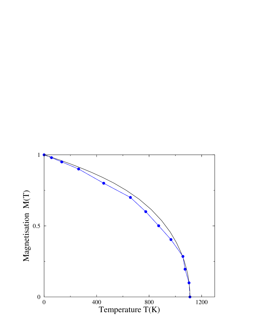
Figure 1: The magnetisation of FePt versus temperature. The filled circles refer to a magnetisation along $\hat{n}=(1,0,1)$. $T_{c}$ is at 1105K with the easy axis, $(0,0,1)$. The full line shows the mean field approximation to a classical Heisenberg model for comparison.

Figure 2 shows the magnetic anisotropy energy, $\Delta F((0,0,1),(1,0,0))=-(K_{2}+K_{4})$ versus the square of the magnetisation. The same linear relationship that we found for $FePt$ MAEvsT is evident, a clear consequence of the itinerant nature of the magnetism is this system. This magnetisation dependence differs significantly from that produced by the single ion model, also shown in the figure. At $T=0$K, $K_{2}+K_{4}$ is 0.335meV is in fair agreement with the value of 0.45 meV inferred from low temperature measurements on well ordered samples FePd-expt (as with $FePt$, $K$ decreases significantly if the degree of long-range chemical order is reduced). The value is also in line with values of 0.1 to 0.5 meV found by other ab-initio approaches  FePd-theory .

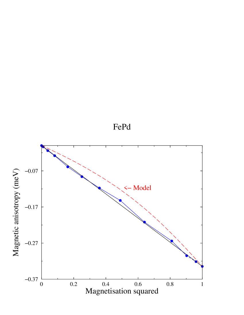
Figure 2: The magnetic anisotropy of FePd as a function of the square of magnetisation. The filled circles show the calculations from the ab-initio theory, the full line $K_{0}(m(T)/m(0))^{2}$ and the dashed line the single-ion model function $K_{0}<g_{2}(\hat{e})>_{T}/<g_{2}(\hat{e})>_{0}$ with $K_{0}=$ -0.335meV.

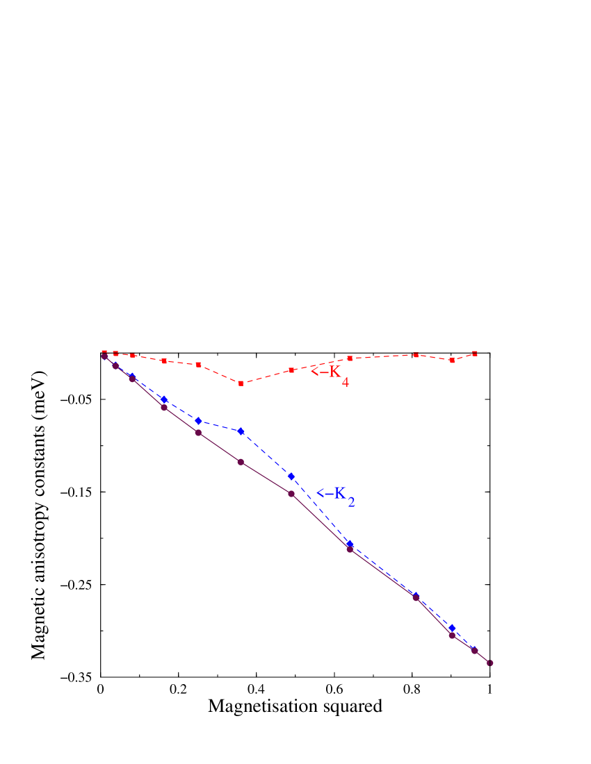
Figure 3: The magnetic anisotropy constants $K_{2}$, $K_{4}$ of FePd as a function of the square of magnetisation. The filled circles and full line show the calculations from the ab-initio theory of the sum, the dashed line with filled diamonds describes $K_{2}$ and the dotted line with squares shows $K_{4}$.

From $T_{\vartheta}$ for both $\vartheta=\frac{\pi}{4}$,$\varphi=0$ and $\vartheta=\frac{\pi}{3}$,$\varphi=0$ the magnitudes of the MCA constants $K_{2}$ and $K_{4}$ are extracted and shown in Figure 3. The dominance of $K_{2}$ is obvious but it is also clear that the $m^{2}$ dependence is followed closely by the total anisotropy, $K_{2}+K_{4}$, and only approximately by the leading constant $K_{2}$. It is interesting to note that an anisotropic classical Heisenberg model leads to similar $m$ dependence to $K$ if treated within a mean field approach. To illustrate this point we show in Figure 4 the results of mean field calculations of $K$ for a model with both single-ion and anisotropic nearest neighbor exchange,i.e. where the following hamiltonian is appropriate:

$$H=-\frac{1}{2}\sum_{i,j}(J^{\|}(e_{x,i}e_{x,j}+e_{y,i}e_{y,j})+J^{\bot}e_{z,i}e_{z,j})-k\sum_{i}(e_{z,i})^{2}$$ (67)

The full curve shows the single ion model results for the limit $J^{\|}=J^{\bot}$, which are also shown in Figure 3. At low $T$ as $m(T)\rightarrow 1$, $K(T)/K(0)$ has the familiar $m^{l(l+1)/2}$ form with $l=1$ for a uniaxial magnet. By introducing a small difference between $J^{\|}$ and $J^{\bot}$, so that $J^{\bot}-J^{\|}=0.01J^{\bot}$, $K(T)/K(0)$ varies as $m^{2}$.

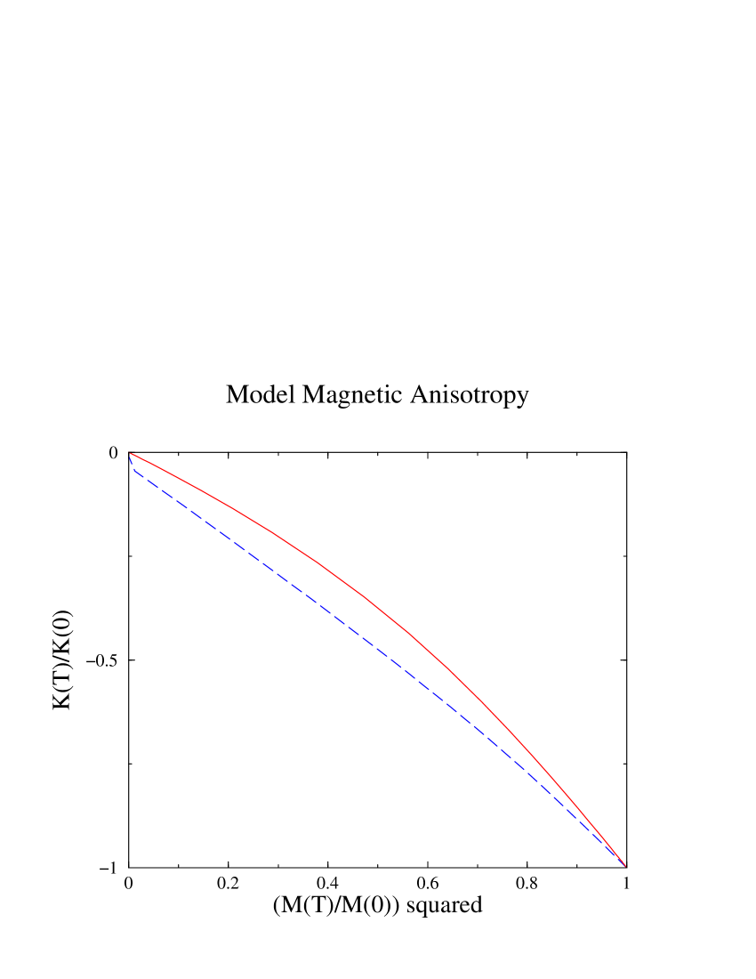
Figure 4: The magnetic anisotropy energy $K$ calculated in a mean field approximation for a model of a uniaxial magnet which has both anisotropic exchange and single ion anisotropy. The full line shows results with single ion anisotropy only, $k=0.002J^{\bot}$ and $J^{\bot}-J^{\|}=0$. The dashed line shows results for the same $k$ and $J^{\bot}-J^{\|}=0.01J^{\bot}$.

IX CUBIC MAGNETIC ANISOTROPY - THE F.C.C. $Fe_{50}Pt_{50}$ SOLID SOLUTION

Crystal structure is known to have a profound effect upon the magnetic anisotropy. Magnetic anisotropy within a single ion anisotropy model decreases according to $m^{l(l+1)/2}$ at low $T$, ($m\approx 1$) and proportional to $m^{l}$ for small $m$ at higher $T$. For materials with tetragonal symmetry, $l=2$ as shown in Fig.2. On this basis a cubic magnet’s $K$ should possess an $m$ dependence where $l=4$, i.e. $m^{10}$ at low $T$ and $m^{4}$ at higher $T$. In this section we show our results for the itinerant magnet, compositionally disordered $Fe_{50}Pt_{50}$. In this system the lattice sites of the f.c.c. lattice are occupied at random by either $Fe$ or $Pt$ atoms. The cubic symmetry causes this alloy to be magnetically very soft. Ordering into a tetragonal $L1_{0}$ structure of layers of predominantly $Fe$ atoms stacked alternately with $Pt$ layers along the $(1,0,0)$ direction causes a significant increase of $K$. Okamoto et al Okamoto have measured $K$ of $FePt$ carefully as a function of compositional order and the trend, for $T=0$K, has been successfully reproduced in ab-initio calculations ICNDR ; Burkert .

As with our earlier calculations for $L1_{0}$-FePt MAEvsT and FePd, this disordered alloy’s magnetisation follows a similar T-dependence to that of a mean field treatment of a classical Heisenberg model. We find a Curie temperature of 1085K, again a mean field value which is in reasonable agreement with the experimental value of 750K Okamoto . Figure 5 shows our calculations of the magnetisation dependence of the leading magnetic anisotropy constant $K_{1}$ (Eq.7). At $T=0$K, $\Delta F((0,0,1),(1,1,1))=-K_{1}/3$ is just 2.8$\mu$eV ($\pm 0.1\mu$eV) , some three orders of magnitude smaller than the uniaxial MCA ($K_{2}+K_{4}$) we find its $L1_{0}$-ordered counterpart MAEvsT . Despite this small value we find that our method is robust enough to follow the magnetisation and $T$-dependence of $K_{1}$. $K_{1}$ is determined from a calculation of $T_{\varphi}$ where for $\vartheta=\pi/2$ and $\varphi=\pi/8$ it equals $K_{1}/2$. As expected $K_{1}$ decreases rapidly - Fig. 5 depicts $K_{1}$ versus the fourth power of the magnetisation. At low $T$ $K_{1}$ varies approximately as $m^{7}$ whereas this dependence becomes $m^{4}$ for smaller $M$ and higher $T$. Fig.5 also shows the behavior of the single ion model for a cubic system for comparison. As with the uniaxial metallic magnets already investigated, the ab-initio R-DLM results differ significantly.

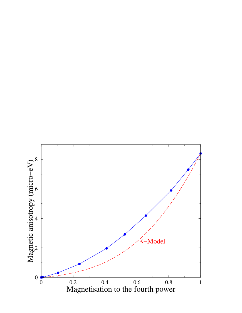
Figure 5: The magnetic anisotropy constant $K_{1}$ of the cubic magnet $Fe_{50}Pt_{50}$ as a function of the fourth power of the magnetisation, $m^{4}$. The filled circles show the calculations from the ab-initio theory and the dashed line the single-ion model function $K_{1}^{0}<g_{2}(\hat{e})>_{T}/<g_{2}(\hat{e})>_{0}$ with $K_{1}^{0}=$ 8.4$\mu$eV.

X CONCLUSIONS

We have shown that by including relativistic effects such as spin-orbit coupling into the Disordered Local Moment theory of finite temperature magnetism, the temperature dependence of magnetic anisotropy can be obtained. Magnetic anisotropy is determined via consideration of magnetic torque expressed within a multiple-scattering formalism. For uniaxial metallic magnets with tetragonal crystal symmetry, $L1_{0}$-$FePt$ and $FePd$, we find $K$ to vary with the square of the overall magnetisation, $m(T)$. This is at odds with what an analysis based on a single ion anisotropy model would find but in agreement with experimental measurements for $FePt$. An interpretation in terms of an anisotropic Heisenberg model explains this behavior Mryasov . We suggest that this $m^{2}$ behavior is typical for high $T_{c}$ transition metal alloys ordered into a tetragonal structure. We find the first anisotropy coefficient, $K_{2}$ to be dominant. We have also investigated the magnetic anisotropy of metallic magnets with cubic crystal symmetry which are very soft magnetically. In the example of the f.c.c. substitutional alloy, $Fe_{50}Pt_{50}$, the leading constant $K_{1}$ decreases according to $m^{n}$ where $n$ ranges between 7 and 4 as the temperature is increased. This behavior also differs significantly from that of a simple single ion model. Application of this R-DLM theory of magnetism at finite temperature has been confined here to bulk crystalline systems. It also, however, has particular relevance for thin film and nanostructured metallic magnets SKKR ; Antoniak ; Ebert where it can be used to uncover temperature-induced reorientation transitions. e.g. Buruzs et al. Laszlo have recently applied the theory to $Fe$ and $Co$ monolayers on $Cu(111)$. Future possible applications also include the study of the temperature dependence of magnetostriction, the design of high permeability materials and magnetotransport phenomena in spintronics.

XI Acknowledgements

We acknowledge support from the EPSRC(U.K), the Centre for Scientific Computing at the University of Warwick, the Hungarian National Science Foundation (OKTA T046267) and to the Center for Computational Materials Science (Contract No. FWF W004 and GZ 45.547).

APPENDIX A: TORQUE FOR $T\rightarrow 0$K

Concerning the MCA of a ferromagnet at $T=0$K, the relevant part of the total energy is

$$F^{(\widehat{n})}=-\int d\varepsilon\,f_{FD}\left(\varepsilon;\nu^{\left(\widehat{n}\right)}\right)\,N^{\left(\widehat{n}\right)}\left(\varepsilon\right)$$ (68)

where $N^{\left(\widehat{n}\right)}\left(\varepsilon\right)$ is the integrated density of states,

$$N^{\left(\widehat{n}\right)}\left(\varepsilon\right)=N_{0}\left(\varepsilon\right)-\frac{1}{\pi}\operatorname{Im}\ln\det\left(\underline{\underline{t}}\left(\widehat{n};\varepsilon\right)^{-1}-\underline{\underline{G}}_{0}\left(\varepsilon\right)\right),$$ (69)

and the inverse of the single site t-matrix is

$$\underline{t}_{i}\left(\widehat{n};\varepsilon\right)=\underline{R}\left(\widehat{n}\right)\,\underline{t}_{i}\left(\widehat{z};\varepsilon\right)\underline{R}\left(\widehat{n}\right)^{+}.$$ (70)

Now $\underline{R}\left(\widehat{n}\right)=\exp i\alpha_{\widehat{m}}(\widehat{m}\cdot\vec{\underline{J}})$ where $\alpha_{\widehat{m}}$ is the angle of rotation about an axis $\widehat{m}=(\widehat{z}\wedge\widehat{n})/|\widehat{z}\wedge\widehat{n}|$ and $\vec{\underline{J}}$ is the total angular momentum. The torque quantity $T_{\alpha_{\widehat{u}}}^{\left(\widehat{n}\right)}=-\frac{\partial F^{(\widehat{n})}}{\partial\alpha_{\widehat{u}}}$, describing the variation of the total energy with respect to a rotation of the magnetisation about an axis $\widehat{u}$, is

$$T_{\alpha_{\widehat{u}}}^{\left(\widehat{n}\right)}=-\frac{1}{\pi}\int d\varepsilon\,f_{FD}\left(\varepsilon;\nu^{\left(\widehat{n}\right)}\right)\operatorname{Im}\frac{\partial}{\partial\alpha_{\widehat{u}}}\left[\ln\det\left(\underline{\underline{t}}\left(\widehat{n};\varepsilon\right)^{-1}-\underline{\underline{G}}_{0}\left(\varepsilon\right)\right)\right]$$ (71)

which can be written

$$T_{\alpha_{\widehat{u}}}^{\left(\widehat{n}\right)}=-\frac{1}{\pi}\int d\varepsilon\,f_{FD}\left(\varepsilon;\nu^{\left(\widehat{n}\right)}\right)\operatorname{Im}\sum_{i}tr\left(\underline{\tau}^{\left(\widehat{n}\right)}_{ii}\left(\varepsilon\right)\frac{\partial}{\partial\alpha_{\widehat{u}}}\left(\underline{R}\left(\widehat{n}\right)\underline{t}\left(\widehat{n};\varepsilon\right)^{-1}\underline{R}\left(\widehat{n}\right)^{+}\right)\right).$$ (72)

Since $\frac{\partial\underline{R}\left(\widehat{n}\right)}{\partial\alpha_{\widehat{u}}}=i(\vec{\underline{J}}\cdot\widehat{u})\underline{R}\left(\widehat{n}\right)$ and $\frac{\partial\underline{R}\left(\widehat{n}\right)^{+}}{\partial\alpha_{\widehat{u}}}=-i(\vec{\underline{J}}\cdot\widehat{u})\underline{R}\left(\widehat{n}\right)$,

$$T_{\alpha_{\widehat{u}}}^{\left(\widehat{n}\right)}=\frac{1}{\pi}\int d\varepsilon\,f_{FD}\left(\varepsilon;\nu^{\left(\widehat{n}\right)}\right)\operatorname{Im}i\,\sum_{i}tr\left(\underline{\tau}^{\left(\widehat{n}\right)}_{ii}\left(\varepsilon\right)\left[(\vec{\underline{J}}\cdot\widehat{u})\underline{t}\left(\widehat{n};\varepsilon\right)^{-1}-\underline{t}\left(\widehat{n};\varepsilon\right)^{-1}(\vec{\underline{J}}\cdot\widehat{u})\right]\right).$$ (73)

For $T_{\vartheta(\varphi)}^{\left(\widehat{n}\right)}$, $(\vec{\underline{J}}\cdot\widehat{u})$ is just $\underline{J}_{y(z)}$.

Consider now our finite temperature torque expression, Eq.(65), i.e.

$$T_{\alpha}=\frac{\operatorname{Im}}{\pi}\int d\varepsilon\,f_{FD}\left(\varepsilon;\nu^{\left(\widehat{n}\right)}\right)\sum_{i}\int\frac{\partial P_{i}^{\left(\widehat{n}\right)}\left(\widehat{e}_{i}\right)}{\partial\alpha}\ln\det\underline{M}_{i}^{\left(\widehat{n}\right)}\left(\varepsilon;\widehat{e}_{i}\right)d\widehat{e}_{i}\;,$$ (74)

with $\alpha=\vartheta$ or $\varphi$ and

$$\underline{M}_{i}^{\left(\widehat{n}\right)}\left(\varepsilon;\widehat{e}_{i}\right)=\underline{I}+\left(\underline{t}_{i}\left(\varepsilon;\widehat{e}_{i}\right)^{-1}-\underline{t}_{i,c}^{\left(\widehat{n}\right)}\left(\varepsilon\right)^{-1}\right)\underline{\tau}_{ii,c}^{\left(\widehat{n}\right)}\left(\varepsilon\right)\;.$$ (75)

By definition,

$$T_{\alpha} =\frac{\operatorname{Im}}{\pi}\int d\varepsilon\,f_{FD}\left(\varepsilon;\nu^{\left(\widehat{n}\right)}\right)\sum_{i}\int\lim_{\Delta\alpha\rightarrow 0}\frac{P_{i}^{\left(\widehat{n}+\Delta\widehat{n}\right)}\left(\widehat{e}_{i}\right)-P_{i}^{\left(\widehat{n}\right)}\left(\widehat{e}_{i}\right)}{\Delta\alpha}\ln\det\underline{M}_{i}^{\left(\widehat{n}\right)}\left(\varepsilon;\widehat{e}_{i}\right)d\widehat{e}_{i}$$ (76)

$$=\frac{\operatorname{Im}}{\pi}\int d\varepsilon\,f_{FD}\left(\varepsilon;\nu^{\left(\widehat{n}\right)}\right)\sum_{i}\lim_{\Delta\alpha\rightarrow 0}\frac{1}{\Delta\alpha}\left\{\int P_{i}^{\left(\widehat{n}+\Delta\widehat{n}\right)}\left(\widehat{e}_{i}\right)\ln\det\underline{M}_{i}^{\left(\widehat{n}\right)}\left(\varepsilon;\widehat{e}_{i}\right)d\widehat{e}_{i}\right.$$ (77)

$$\begin{array}[c]{cccccccc}&&&&&&&\end{array}\;\left.-\int P_{i}^{\left(\widehat{n}\right)}\left(\widehat{e}_{i}\right)\ln\det\underline{M}_{i}^{\left(\widehat{n}\right)}\left(\varepsilon;\widehat{e}_{i}\right)d\widehat{e}_{i}\right\}\;.$$ (79)

Approaching $T=0$,

$$P_{i}^{\left(\widehat{n}\right)}\left(\widehat{e}_{i}\right)\rightarrow\delta\left(\widehat{n}-\widehat{e}_{i}\right)\;,\;\underline{t}_{i}\left(\varepsilon;\widehat{e}_{i}\right)\rightarrow\underline{t}_{i}\left(\varepsilon;\widehat{n}\right)\;,$$ (80)

$$P_{i}^{\left(\widehat{n}+\Delta\widehat{n}\right)}\left(\widehat{e}_{i}\right)\rightarrow\delta\left(\widehat{n}+\Delta\widehat{n}-\widehat{e}_{i}\right)\;,\;\underline{t}_{i}\left(\varepsilon;\widehat{e}_{i}\right)\rightarrow\underline{t}_{i}\left(\varepsilon;\widehat{n}+\Delta\widehat{n}\right)\;,$$ (81)

while

$$\ln\det\underline{M}_{i}^{\left(\widehat{n}\right)}\left(\varepsilon;\widehat{e}_{i}\right)\rightarrow Tr\left(\left[\underline{t}_{i}\left(\varepsilon;\widehat{e}_{i}\right)^{-1}-\underline{t}_{i}^{\left(\widehat{n}\right)}\left(\varepsilon\right)^{-1}\right]\underline{\tau}_{ii}^{\left(\widehat{n}\right)}\left(\varepsilon\right)\right)\;.$$ (82)

Therefore,

$$T_{\alpha} =\frac{\operatorname{Im}}{\pi}\int d\varepsilon\,f_{FD}\left(\varepsilon;\nu^{\left(\widehat{n}\right)}\right)\sum_{i}\lim_{\Delta\alpha\rightarrow 0}\frac{1}{\Delta\alpha}\times$$ (83)

$$Tr\left(\left[\underline{t}_{i}\left(\varepsilon;\widehat{n}+\Delta\widehat{n}\right)^{-1}-\underline{t}_{i}^{\left(\widehat{n}\right)}\left(\varepsilon\right)^{-1}\right]\underline{\tau}_{ii,c}^{\left(\widehat{n}\right)}\left(\varepsilon\right)\right)-Tr\left(\left[\underline{t}_{i}\left(\varepsilon;\widehat{n}\right)^{-1}-\underline{t}_{i}^{\left(\widehat{n}\right)}\left(\varepsilon\right)^{-1}\right]\underline{\tau}_{ii}^{\left(\widehat{n}\right)}\left(\varepsilon\right)\right)$$ (84)

$$=\frac{\operatorname{Im}}{\pi}\int d\varepsilon\,f_{FD}\left(\varepsilon;\nu^{\left(\widehat{n}\right)}\right)\sum_{i}\lim_{\Delta\alpha\rightarrow 0}\frac{1}{\Delta\alpha}Tr\left(\left[\underline{t}_{i}\left(\varepsilon;\widehat{n}+\Delta\widehat{n}\right)^{-1}-\underline{t}_{i}\left(\varepsilon;\widehat{n}\right)^{-1}\right]\underline{\tau}_{ii}^{\left(\widehat{n}\right)}\left(\varepsilon\right)\right)$$ (85)

$$=\frac{\operatorname{Im}}{\pi}\int d\varepsilon\,f_{FD}\left(\varepsilon;\nu^{\left(\widehat{n}\right)}\right)\sum_{i}Tr\left(\frac{\partial\underline{t}_{i}\left(\varepsilon;\widehat{n}\right)^{-1}}{\partial\alpha}\underline{\tau}_{ii}^{\left(\widehat{n}\right)}\left(\varepsilon\right)\right)\;,$$ (86)

which is equivalent to Eq.(72).

References

- (1) H.J.F.Jansen, Phys. Rev. B 59, 4699 (1999).
- (2) J.Kubler, Theory of itinerant electron magnetism, (Oxford: Clarendon 2000).
- (3) J.B.Staunton, Rep.Prog. Phys. 57, 1289, (1994).
- (4) S.S.A.Razee et al., Phys. Rev. Lett. 82, 5369, (1999).
- (5) A.B.Shick et al., Phys. Rev. B 56, R14259, (1997).
- (6) T.Burkert et al.,Phys. Rev. B 69, 104426, (2004).
- (7) B.Lazarovits et al.,J. Phys.: Cond. Matt.16, S5833, (2004).
- (8) X.Qian and W.Hubner, Phys. Rev. B 64, 092402, (2001).
- (9) I.Cabria et al., Phys. Rev. B 63, 104424, (2001).
- (10) e.g. H.Kronmuller et al., J.Mag.Magn.Mat. 175, 177, (1997); M.E.Schabes, J.Mag.Magn.Mat. 95, 249-288, (1991).
- (11) D.V.Baxter et al., Phys.Rev. B 65, 212407, (2002); K.Hamaya et al., J.Appl.Phys. 94, 7657-61, (2003); A.B.Shick et al., Phys.Rev. B 73, 024418, (2006).
- (12) H.B.Callen and E.Callen, J.Phys.Chem.Solids, 27, 1271, (1966); N.Akulov, Z. Phys. 100, 197, (1936); C.Zener, Phys. Rev. B96, 1335, (1954).
- (13) J.B.Staunton et al., Phys. Rev. Lett. 93, 257204, (2004).
- (14) O.Mryasov et al., Europhys.Lett. 69, 805, (2005); R.Skomski et al., J. Appl. Phys. 99, 08E916, (2006).
- (15) X.W.Wu et al., Appl. Phys. Lett. 82, 3475, (2003).
- (16) J.-U.Thiele et al., J. Appl. Phys. 91, 6595, (2002).
- (17) S.Okamoto et al., Phys. Rev. B66, 024413, (2002).
- (18) Electron Correlations and Magnetism in Narrow Band System, edited by T. Moriya (Springer, N.Y., 1981).
- (19) B.L.Gyorffy et al., J. Phys. F: Met. Phys. 15, 1337 (1985).
- (20) J.B.Staunton and B.L.Gyorffy, Phys. Rev. Lett. 69, 371 (1992).
- (21) S.Sun et al., Science 287, 1989, (2000).
- (22) R.C.O’Handley, Modern Magnetic Materials, (Wiley, 2000).
- (23) A.Lyberatos and K.Y.Guslienko, J. Appl. Phys. 94, 1119, (2003); H.Saga et al., Jpn. J. Appl. Phys. Part 1 38, 1839, (1999); M.Alex et al., IEEE Trans. Magn. 37, 1244, (2001).
- (24) O.A.Ivanov et al., Fiz. Met. Metalloved. 35, 92, (1973.
- (25) R.F.Farrow et al., J. Appl. Phys. 79, 5967,(1996)..
- (26) S.S.A.Razee et al., Phys. Rev. B56, 8082 (1997).
- (27) S.Ostanin et al., Phys. Rev. B69, 064425, (2004).
- (28) S.Ostanin et al., J.Appl.Phys.93, 453, (2003); J.B.Staunton et al.,J. Phys.: Cond. Matt.16, S5623, (2004).
- (29) X.Wang et al., Phys. Rev. B 54, 61-64, (1996).
- (30) A.I. Akhiezer, V.G.Baryakhtar and S.V.Peletminskii, Spin Waves and Magnetic Excitations, (Amsterdam: North Holland), (1968).
- (31) E.Bruno and B.Ginatempo, Phys. Rev. B55, 12946, (1997).
- (32) J.Korringa, Physica 13, 392, (1947); W.Kohn and N.Rostoker, Phys.Rev. 94, 1111, (1954).
- (33) G.M.Stocks et al., Phys. Rev. Lett. 41, 34, (1978).
- (34) G.M.Stocks and H.Winter, Z.Phys.B 46, 95, (1982); D.D.Johnson et al., Phys. Rev. Lett. 56, 2088, (1986).
- (35) S.S.A. Razee et al., Phys. Rev. Lett. 88, 147201, (2002).
- (36) M.F.Ling et al., Europhys.Lett. 25, 631, (1994).
- (37) J.B.Staunton et al.,J. Phys.: Cond. Matt. 9, 1281-1300, (1997).
- (38) V.Crisan et al., Phys. Rev. B 66, 014416, (2002).
- (39) M.Lueders et al., Phys. Rev. B 71, 205109, (2005).
- (40) I.Hughes et al., in preparation.
- (41) K.Sato et al., J. Phys.: Cond. Matt. 16, S5491, (2004).
- (42) A.M.N.Niklasson et al., Phys. Rev. B 67, 235105, (2003).
- (43) D.A.Rowlands et al., Phys. Rev. B 67, 115109, (2003).
- (44) D.A.Rowlands et al., Phys. Rev. B 73, 165122, (2006).
- (45) R.P.Feynman, Phys. Rev. 97, 660, (1955).
- (46) P.Soven, Phys.Rev. 156, 809, (1967).
- (47) A.Messiah, Quantum Mechanics, (Amsterdam: North Holland), (1965).
- (48) P.Strange et al., J.Phys. C 17, 3355-71, (1984).
- (49) B.L.Gyorffy and M.J.Stott, in Band Structure Spectroscopy of Metals and Alloys, eds.: D.J.Fabian and L.M.Watson, (Academic Press, New York), (1973).
- (50) B.Ginatempo and J.B.Staunton, J.Phys.F 18, 1827-37, (1988).
- (51) P.Lloyd and P.R.Best, J.Phys.C 8, 3752, (1975).
- (52) J.S.Faulkner and G.M.Stocks, Phys. Rev. B 21, 3222, (1980).
- (53) A.Buruzs et al., submitted to J.Mag.Magn.Mat. (2006).
- (54) J.B.Staunton et al., Phys. Rev. B 62, 1075-82, (2000).
- (55) L.Wang et al., J.Appl.Phys. 95, 7483-5, (2004).
- (56) A.Ye.Yermakov et al., Fiz. Met. Metall. 69, Pt.5, 198, (1990); H.Shima et al., J. Mag. Magn. Mat. 272, Part 3, 2173, (2004)
- (57) G.H.O.Daalderop et al., Phys. Rev. B 44, 12054, (1991); I.V.Solovyev et al., Phys. Rev. B 52, 13419, (1995); I.Galanakis et al., Phys. Rev. B 62, 6475, (2000); D.Garcia et al., Phys. Rev. B 63, 104421, (2001).
- (58) T.Burkert et al., Phys. Rev. B 71, 134411, (2005).
- (59) C.Antoniak et al., Europhys.Lett. 70, 250-6, (2005).
- (60) J.Zabloudil et al. in Electron Scattering in Solid Matter, Springer Series in Solid State Sciences, 147 (Springer, Heidelberg, 2005).
- (61) H.Ebert et al.,Comp. Mat. Sci. 35, 279-282, (2006).