Non-Fermi liquid behavior in transport across carbon nanotube quantum dots

Leonhard Mayrhofer and Milena Grifoni Theoretische Physik, UniversitΓ€t Regensburg, 93040 Germany
Abstract

A low energy-theory for non-linear transport in finite-size single-wall carbon nanotubes, based on a microscopic model for the interacting $p_{z}$ electrons and successive bosonization, is presented. Due to the multiple degeneracy of the energy spectrum diagonal as well as off-diagonal (coherences) elements of the reduced density matrix contribute to the nonlinear transport. A four-electron periodicity with a characteristic ratio between adjacent peaks, as well as nonlinear transport features, in quantitative agreement with recent experiments, are predicted.

pacs:
PACS numbers: 73.63.Fg, 71.10.Pm, 73.23.Hk

Since their recent discovery single-wall carbon nanotubes (SWNTs), cf. e.g. Saito1998 , have attracted a lot of experimental and theoretical attention. In particular, as suggested in the seminal works Egger1997 ; Kane1997 , due to the peculiar one-dimensional character of their electronic bands, metallic SWNTs are expected to exhibit Luttinger liquid behavior at low energies, reflected in power-law dependence of various quantities and spin-charge separation. Later experimental observations have provided a confirmation of the theory Bockrath1999 ; Postma2001 . As typical of interacting electron systems in reduced dimension, SWNTs weakly coupled to leads exhibit Coulomb blockade at low temperatures Tans1997 with characteristic even-odd Cobden2002 or four-fold periodicity Liang2002 ; Sapmaz2005 ; Moriyama2005 . In Sapmaz2005 not only the ground state, but also several excited states could be seen in stability diagrams of closed SWNT quantum dots. Such two-fold and four-fold character can be qualitatively understood from symmetry arguments related to the two-fold band degeneracy of SWNTs and the inclusion of the spin degree of freedom. So far, a quantitative description has relied on density functional theory calculations Ke2003 or on a mean field description of the Coulomb blockade Oreg2000 . In particular, the position of the spectral lines in the stability diagram measured in Sapmaz2005 was found to be in quantitative agreement with the predictions in Oreg2000 . However, a mean field description may be not justified for one-dimensional systems. For example, to describe the spectral lines of the sample with four-fold periodicity (sample C) in Sapmaz2005 , a quite peculiar choice of the mean field parameters was made, and a quantum dot length three times shorter than the measured SWNT length was assumed. Moreover, to date no quantitative calculation of the nonlinear current across a SWNT dot has been provided.

In this Letter we investigate spectral as well as dynamical properties of electrons in metallic SWNT quantum dots at low energies. We start from a microscopic description of metallic SWNTs and include Coulomb interaction effects, beyond mean-field, by using bosonization techniques Egger1997 ; Kane1997 , yielding the spectrum and eigenfunctions of the isolated finite length SWNT. Due to the many-fold degeneracies of the spectrum, the current-voltage characteristics is obtained by solving equations of motion for the reduced density matrix (RDM) including off-diagonal elements. Analytical results for the conductance are provided, which account for the different heights of the conductance peaks in Sapmaz2005 . Moreover, we can quantitatively reproduce all the spectral lines seen in sample C in Sapmaz2005 by solely using the two ground state addition energies provided in that work. The derived level spacing is in agreement with the measured SWNT length.

To start with, we consider the total Hamiltonian

$$H=H_{\odot}+H_{s}+H_{d}+H_{T}+H_{\rm gate},$$ (1)

where $H_{\odot}$ is the interacting SWNT Hamiltonian (cf. Eq. (Non-Fermi liquid behavior in transport across carbon nanotube quantum dots) below) and $H_{s/d}$ describe the isolated metallic source and drain contacts as a thermal reservoir of non-interacting quasi-particles. Upon absorbing terms proportional to external source and drain voltages $V_{s/d}$, they read ($l=s,d$) Hl=βˆ‘Οƒβ€‹qβ†’Ξ΅qβ†’,l​cq→​σ​l†​cq→​σ​lsubscript𝐻𝑙subscriptπœŽβ†’π‘žsubscriptπœ€β†’π‘žπ‘™superscriptsubscriptπ‘β†’π‘žπœŽπ‘™β€ subscriptπ‘β†’π‘žπœŽπ‘™H_{l}=\sum_{\sigma\vec{q}}\varepsilon_{\vec{q},l}c_{\vec{q}\sigma l}^{\dagger}c_{\vec{q}\sigma l}, where cq→​σ​l†superscriptsubscriptπ‘β†’π‘žπœŽπ‘™β€ c_{\vec{q}\sigma l}^{\dagger} creates a quasi-particle with spin $\sigma$ and energy $\varepsilon_{\vec{q},l}=\varepsilon_{\vec{q}}-eV_{s/d}$ in lead $s/d$. The transfer of electrons between the leads and the SWNT is taken into account by

HT=βˆ‘l=s,dβˆ‘Οƒβˆ«d3​r​(Tl​(rβ†’)​Ψσ†​(rβ†’)​Φσ​l​(rβ†’)+h.c.),subscript𝐻𝑇subscript𝑙𝑠𝑑subscript𝜎superscriptd3π‘Ÿsubscriptπ‘‡π‘™β†’π‘ŸsuperscriptsubscriptΞ¨πœŽβ€ β†’π‘ŸsubscriptΞ¦πœŽπ‘™β†’π‘Ÿh.c.H_{T}=\sum_{l=s,d}\sum_{\sigma}\int\textrm{d}^{3}r\left(T_{l}(\vec{r})\Psi_{\sigma}^{\dagger}(\vec{r})\Phi_{\sigma l}(\vec{r})+\textrm{h.c.}\right), (2)

where Ψσ†superscriptsubscriptΞ¨πœŽβ€ \Psi_{\sigma}^{\dagger} and Φσ​l†​(rβ†’)=βˆ‘qβ†’Ο•qβ†’βˆ—β€‹(rβ†’)​cq→​σ​l†superscriptsubscriptΞ¦πœŽπ‘™β€ β†’π‘Ÿsubscriptβ†’π‘žsuperscriptsubscriptitalic-Ο•β†’π‘žβ†’π‘Ÿsuperscriptsubscriptπ‘β†’π‘žπœŽπ‘™β€ \Phi_{\sigma l}^{\dagger}(\vec{r})=\sum_{\vec{q}}\phi_{\vec{q}}^{*}(\vec{r})c_{\vec{q}\sigma l}^{\dagger} are electron creation operators in the SWNT and in lead $l$, respectively, and $T_{l}(\vec{r})$ describes the transparency of the tunneling contact $l$. Finally, $H_{\rm gate}=-\mu_{g}{\cal N}_{c}$ accounts for a gate voltage capacitively coupled to the SWNT, with ${\cal N}_{c}$ counting the total electron number in the SWNT.
SWNT Hamiltonian. In the following the focus is on armchair SWNTs at low energies. Then, if periodic boundary conditions are applied, only the gapless energy sub-bands nearby the Fermi points F=Β±Kβ†’0=Β±K0​e^x𝐹plus-or-minussubscript→𝐾0plus-or-minussubscript𝐾0subscript^𝑒π‘₯F=\pm{\vec{K}_{0}}=\pm K_{0}\hat{e}_{x} with e^xsubscript^𝑒π‘₯{\hat{e}_{x}} along the nanotube axis, are relevant Egger1997 ; Kane1997 . To each Fermi point two different branches r=R/Lπ‘Ÿπ‘…πΏr=R/L are associated to the Bloch waves Ο†R/L,F,κ​(rβ†’)=ei​κ​x​φR/L,F​(rβ†’)subscriptπœ‘π‘…πΏπΉπœ…β†’π‘Ÿsuperscriptπ‘’π‘–πœ…π‘₯subscriptπœ‘π‘…πΏπΉβ†’π‘Ÿ\varphi_{R/L,F,\kappa}(\vec{r})=e^{i\kappa x}\varphi_{R/L,F}(\vec{r}), where ΞΊπœ…\kappa measures the distance from the Fermi points Β±K0plus-or-minussubscript𝐾0\pm K_{0} 
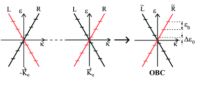
Egger1997 (Fig. 1a left). In this Letter, however, we are interested in finite size effects. Generalizing Fabrizio1995 to the case of SWNTs we introduce standing waves which fulfill open boundary conditions (Fig. 1a right):

$$\varphi^{OBC}_{{\tilde{R}/\tilde{L}},\kappa}(\vec{r})=\frac{1}{\sqrt{2}}\left[\varphi_{R/L,K_{0},\kappa}(\vec{r})-\varphi_{L/R,-K_{0},-\kappa}(\vec{r})\right]\;,$$ (3)

with quantization condition $\kappa=\pi(m_{\kappa}+\Delta)/L$, $m_{\kappa}$ an integer, and $L$ the SWNT length. The offset parameter $\Delta$ occurs if $K_{0}\neq\pi n/L$, and is responsible for the energy mismatch between the $\tilde{R}$ and $\tilde{L}$ branches. Including the spin degree of freedom, the electron operator reads

$$\Psi(\vec{r})=\sum_{\tilde{r}=\tilde{R},\tilde{L}}\sum_{\kappa,\sigma}\varphi_{\tilde{r}\kappa}^{OBC}(\vec{r})c_{\tilde{r}\sigma\kappa}=:\sum_{\sigma}\Psi_{\sigma}(\vec{r})\;,$$ (4)

with $c_{\tilde{r}\sigma\kappa}$ the operator which annihilates $\left|\varphi_{\tilde{r}\kappa}^{OBC}\right\rangle\left|\sigma\right\rangle$. The interacting SWNT Hamiltonian then reads

$\displaystyle H_{\odot}$ $\displaystyle=$ ℏ​vFβ€‹βˆ‘r~​σsgn​(r~)β€‹βˆ‘ΞΊΞΊβ€‹cr~​κ​σ†​cr~​κ​σ+limit-fromPlanck-constant-over-2-pisubscript𝑣𝐹subscript~π‘ŸπœŽsgn~π‘Ÿsubscriptπœ…πœ…superscriptsubscript𝑐~π‘Ÿπœ…πœŽβ€ subscript𝑐~π‘Ÿπœ…πœŽ\displaystyle\hbar v_{F}\sum_{\tilde{r}\sigma}\textrm{sgn}(\tilde{r})\sum_{\kappa}\kappa c_{\tilde{r}\kappa\sigma}^{\dagger}c_{\tilde{r}\kappa\sigma}+
12β€‹βˆ‘Οƒβ€‹Οƒβ€²βˆ«d3​rβ€‹βˆ«d3​r′​Ψσ†​(rβ†’)​Ψσ′†​(rβ†’β€²)​V​(rβ†’βˆ’rβ†’β€²)​Ψσ′​(rβ†’β€²)​Ψσ​(rβ†’),12subscript𝜎superscriptπœŽβ€²superscript𝑑3π‘Ÿsuperscript𝑑3superscriptπ‘Ÿβ€²superscriptsubscriptΞ¨πœŽβ€ β†’π‘ŸsuperscriptsubscriptΞ¨superscriptπœŽβ€²β€ superscriptβ†’π‘Ÿβ€²π‘‰β†’π‘Ÿsuperscriptβ†’π‘Ÿβ€²subscriptΞ¨superscriptπœŽβ€²superscriptβ†’π‘Ÿβ€²subscriptΞ¨πœŽβ†’π‘Ÿ\displaystyle\!\!\!\!\!\!\!\!\!\!\!\!\!\!\frac{1}{2}\sum_{\sigma\sigma^{\prime}}\int\!d^{3}r\!\int\!d^{3}r^{\prime}\Psi_{\sigma}^{\dagger}(\vec{r})\Psi_{\sigma^{\prime}}^{\dagger}(\vec{r}^{\prime})V(\vec{r}-\vec{r}^{\prime})\Psi_{\sigma^{\prime}}(\vec{r}^{\prime})\Psi_{\sigma}(\vec{r})\;,

with $v_{F}$ the Fermi velocity. We introduce 1D operators

$$\psi_{\tilde{r}F\sigma}(x)=\frac{1}{\sqrt{2L}}\sum_{\kappa}e^{i\textrm{sgn}(F)\kappa x}c_{\tilde{r}\sigma\kappa},$$

in terms of which the electron operator in (4) becomes

$$\Psi_{\sigma}(\vec{r})=\sum_{F,\tilde{r}=\pm}\textrm{sgn}(F)\sqrt{L}{\varphi}_{\textrm{sgn}(F)\tilde{r},F}(\vec{r})\psi_{\tilde{r}F\sigma}(x),$$ (6)

where we used the convention that $R/L=\pm 1$, $\tilde{R}/\tilde{L}=\pm 1$. Upon inserting (6) into (Non-Fermi liquid behavior in transport across carbon nanotube quantum dots), integration over the coordinates perpendicular to the tube axis yields the interacting Hamiltonian expressed in terms of 1D operators and an effective 1D interaction $V_{eff}(x,x^{\prime})$. Using standard bosonization techniques Egger1997 ; Kane1997 $H_{\odot}$ can now be diagonalized when keeping only forward scattering processes associated to $V_{eff}(x,x^{\prime})$.

Refer to caption
Figure 1: Energy spectrum of a SWNT with open boundary conditions (right) described in terms of left ($\tilde{L}$) and right ($\tilde{R}$) branches. It is constructed from suitable combinations of travelling waves whose spectrum is shown on the left side.

It reads

$\displaystyle H_{\odot}$ $\displaystyle=$ $\displaystyle\frac{1}{2}E_{c}\mathcal{N}_{c}^{2}+\varepsilon_{0}\sum_{\tilde{r}\sigma}\left(\frac{\mathcal{N}_{\tilde{r}\sigma}^{2}}{2}+\Delta\textrm{sgn}(\tilde{r})\mathcal{N}_{\tilde{r}\sigma}\right)$ (7)
$\displaystyle+$ βˆ‘q>0βˆ‘j=c,sβˆ‘Ξ΄=Β±Ξ΅j​δ​q​aj​δ​q†​aj​δ​q,subscriptπ‘ž0subscript𝑗𝑐𝑠subscript𝛿plus-or-minussubscriptπœ€π‘—π›Ώπ‘žsuperscriptsubscriptπ‘Žπ‘—π›Ώπ‘žβ€ subscriptπ‘Žπ‘—π›Ώπ‘ž\displaystyle\sum_{q>0}\sum_{j=c,s}\sum_{\delta=\pm}\varepsilon_{j\delta q}a_{j\delta q}^{\dagger}a_{j\delta q}\;,

where the first line is the fermionic contribution and represents the energy cost, due to Pauli’s principle and the Coulomb interaction, of adding new electrons to the system. Specifically, 𝒩r~​σ=βˆ‘ΞΊcr~​σ​κ†​cr~​σ​κ,subscript𝒩~π‘ŸπœŽsubscriptπœ…superscriptsubscript𝑐~π‘ŸπœŽπœ…β€ subscript𝑐~π‘ŸπœŽπœ…\mathcal{N}_{\tilde{r}\sigma}=\sum_{\kappa}c_{\tilde{r}\sigma\kappa}^{\dagger}c_{\tilde{r}\sigma\kappa}, is the operator that counts the number of electrons in the $(\tilde{r}\sigma)$-branch, $\mathcal{N}_{c}=\sum_{\tilde{r}\sigma}\mathcal{N}_{\tilde{r}\sigma}$ yields the total electron number, and $\varepsilon_{0}=\hbar v_{F}\frac{\pi}{L}$ is the free-particle level spacing (see Fig. 1). The term $E_{c}=W_{00}$ is the SWNT charging energy, where $W_{qq}=\frac{1}{L^{2}}\int_{0}^{L}dx\int_{0}^{L}dx^{\prime}V_{eff}(x,x^{\prime})\cos(qx)\cos(qx^{\prime})$. The second line of (7) describes bosonic excitations in terms of the bosonic operators $a_{j\delta q}$. Four channels are associated to total ($j\delta=c+$, $s+$) and relative $(j\delta=c-,s-)$ (with respect to the occupation of the $\tilde{R}$ and $\tilde{L}$ branch) charge and spin excitations. Generalized spin-charge separation occurs, since for three of the channels the energy dispersion is the same as for the noninteracting system, $\varepsilon_{j\delta q}=\hbar v_{F}q=\hbar v_{F}\frac{\pi}{L}n_{q}=:\varepsilon_{0}n_{q}$, ($n_{q}$ a positive integer), but the $(c+)$ channel is affected by the interaction with $\varepsilon_{c+\,q}=\varepsilon_{0}n_{q}(1+8W_{qq}/\varepsilon_{0})^{1/2}$. The eigenstates are

$$\prod_{q>0,j\delta}\left(m_{j\delta q}!\right)^{-1/2}\left(a{}_{j\delta q}^{\dagger}\right)^{m_{j\delta q}}\left|\vec{N},\vec{0}\right\rangle=:\left|\vec{N},\vec{m}\right\rangle,$$ (8)

where $|\vec{N},\vec{0}\rangle$ has no bosonic excitations and $\vec{N}$ defines the number of electrons in each of the branches $(\tilde{r}\sigma).$

Dynamics. Our starting point to describe transport in SWNTs is the exact equation of motion

iβ€‹β„β€‹βˆ‚ΟI​(t)βˆ‚t=T​rl​e​a​d​s​[HTI​(t),WI​(t)],𝑖Planck-constant-over-2-pisuperscriptπœŒπΌπ‘‘π‘‘π‘‡subscriptπ‘Ÿπ‘™π‘’π‘Žπ‘‘π‘ superscriptsubscript𝐻𝑇𝐼𝑑superscriptπ‘ŠπΌπ‘‘i\hbar\frac{\partial\rho^{I}(t)}{\partial t}=Tr_{leads}\left[H_{T}^{I}(t),W^{I}(t)\right], (9)

for the reduced density matrix (RDM) ρI=T​rl​e​a​d​s​WIsuperscriptπœŒπΌπ‘‡subscriptπ‘Ÿπ‘™π‘’π‘Žπ‘‘π‘ superscriptπ‘ŠπΌ\rho^{I}=Tr_{leads}W^{I} of the SWNT. Here $W^{I}(t)$ is the density matrix of the whole system consisting of the leads and the quantum dot, and T​rl​e​a​d​s𝑇subscriptπ‘Ÿπ‘™π‘’π‘Žπ‘‘π‘ Tr_{leads} indicates the trace over the lead degrees of freedom. The apex $I$ denotes the interaction representation with $H_{T}$ from (2) as the perturbation. We make the following approximations: i) We assume weak coupling to the leads, and treat $H_{T}$ up to second order, i.e., we consider the leads as reservoirs which stay in thermal equilibrium and make the factorization ansatz $W^{I}(t)=\rho^{I}(t)\rho_{s}\rho_{d}=:\rho^{I}(t)\rho_{leads}$ where ρs/d=Zs/dβˆ’1​eβˆ’Ξ²β€‹(Hs/dβˆ’ΞΌs/d​𝒩s/d)subscriptπœŒπ‘ π‘‘superscriptsubscript𝑍𝑠𝑑1superscript𝑒𝛽subscript𝐻𝑠𝑑subscriptπœ‡π‘ π‘‘subscript𝒩𝑠𝑑\rho_{s/d}=Z_{s/d}^{-1}e^{-\beta(H_{s/d}-\mu_{s/d}\mathcal{N}_{s/d})}, with $Z_{s/d}$ the partition function and $\beta$ the inverse temperature. ii) Being interested in long time properties, we can make the so called Markov approximation, where the time evolution of $\dot{\rho}^{I}(t)$ is only local in time. iii) Since we know the eigenstates $|\vec{N},\vec{m}\rangle$ of $H_{\odot}$, it is convenient to calculate the time evolution of $\rho^{I}$ in this basis. We assume that matrix elements between states representing a different number of electrons (charge states) in the SWNT and with different energies vanish. Coherences between degenerate states with the same energy $E$ are retained! Hence we can divide $\rho^{I}(t)$ into block matrices $\rho_{nm}^{I,E_{N}}(t),$ where $E,N$ are the energy and number of particles in the degenerate eigenstates $\left|n\right\rangle$, $\left|m\right\rangle$. We arrive at equations of the Bloch-Redfield form

$$\dot{\rho}_{nm}^{I,E_{N}}(t)=-\sum_{kk^{\prime}}R_{nm\,kk^{\prime}}^{E_{N}}\ \rho_{kk^{\prime}}^{I,E_{N}}(t)\\ +\sum_{E^{\prime}}\sum_{M=N\pm 1}\sum_{kk^{\prime}}R_{nm\,kk^{\prime}}^{E_{N}\,E^{\prime}_{M}}\rho_{kk^{\prime}}^{I,E^{\prime}_{M}}(t),$$ (10)

where $k,k^{\prime}$ run over all degenerate states with fixed particle number. The Redfield tensors are given by $(l=s,d)$

$$R_{nm\,kk^{\prime}}^{E_{N}}=\sum_{l}\sum_{E^{\prime},M,j}\left(\delta_{mk^{\prime}}\Gamma_{l,njjk}^{(+)E_{N}\,E^{\prime}_{M}}+\delta_{nk}\Gamma_{l,k^{\prime}jjm}^{(-)E_{N}\,E^{\prime}_{M}}\right),$$ (11)

and $R_{nm\,kk^{\prime}}^{E_{N}\,E^{\prime}_{M}}=\sum_{l,\alpha=\pm}\Gamma_{l,k^{\prime}mnk}^{(\alpha)E^{\prime}_{M}\,E_{N}}$, where the quantities $\Gamma_{l,njjk}^{(\alpha)E_{N}\,E^{\prime}_{M}}$ are transition rates from a state with $N$ to a state with $M$ particles. Known the stationary density matrix ρs​tIsuperscriptsubscriptπœŒπ‘ π‘‘πΌ\rho_{st}^{I}, the current (through lead $l$) follows from

I=2​R​eβ€‹βˆ‘N,E,Eβ€²βˆ‘n​k​j(Ξ“l,n​j​j​k(+)​EN​EN+1β€²βˆ’Ξ“l,n​j​j​k(+)​EN​ENβˆ’1β€²)​ρk​n,s​tI,EN.𝐼2Resubscript𝑁𝐸superscript𝐸′subscriptπ‘›π‘˜π‘—superscriptsubscriptΞ“π‘™π‘›π‘—π‘—π‘˜subscript𝐸𝑁subscriptsuperscript𝐸′𝑁1superscriptsubscriptΞ“π‘™π‘›π‘—π‘—π‘˜subscript𝐸𝑁subscriptsuperscript𝐸′𝑁1superscriptsubscriptπœŒπ‘˜π‘›π‘ π‘‘πΌsubscript𝐸𝑁I=2{\rm Re}\sum_{N,E,E^{\prime}}\sum_{nkj}\left(\Gamma_{l,njjk}^{(+)E_{N}\,E^{\prime}_{N+1}}-\Gamma_{l,njjk}^{(+)E_{N}\,E^{\prime}_{N-1}}\right)\rho_{kn,st}^{I,E_{N}}. (12)

iv) We exploit the localized character of the transparencies $T_{l}(\vec{r})$ in Eq. (2), and make use of the slowly varying nature of the operator $\psi_{\tilde{r}F\sigma}(x)$ in Eq. (6). This enables us to evaluate the 1D operator at the SWNT contacts and pull it out from the space integrals which enter the definition of the transition rates. It holds ⟨r|ψr~​σ​F​(x=0)|s⟩:=(ψr~​σ)r​sEN​EN+1β€²assignquantum-operator-productπ‘Ÿsubscriptπœ“~π‘ŸπœŽπΉπ‘₯0𝑠superscriptsubscriptsubscriptπœ“~π‘ŸπœŽπ‘Ÿπ‘ subscript𝐸𝑁subscriptsuperscript𝐸′𝑁1\langle r|\psi_{\tilde{r}\sigma F}(x=0)|s\rangle:=\left(\psi_{\tilde{r}\sigma}\right)_{rs}^{E_{N}E^{\prime}_{N+1}}; ⟨r|ψr~​σ​F​(x=L)|s⟩=eβˆ’i​π​sgn​(F)​{𝒩r~​σ​sgn​(r~)+Ξ”}​(ψr~​σ)r​sEN​EN+1β€²quantum-operator-productπ‘Ÿsubscriptπœ“~π‘ŸπœŽπΉπ‘₯𝐿𝑠superscriptπ‘’π‘–πœ‹sgn𝐹subscript𝒩~π‘ŸπœŽsgn~π‘ŸΞ”superscriptsubscriptsubscriptπœ“~π‘ŸπœŽπ‘Ÿπ‘ subscript𝐸𝑁subscriptsuperscript𝐸′𝑁1\langle r|\psi_{\tilde{r}\sigma F}(x=L)|s\rangle=e^{-i\pi{\rm sgn}(F)\{{\cal N}_{\tilde{r}\sigma}{\rm sgn}(\tilde{r})+\Delta\}}\left(\psi_{\tilde{r}\sigma}\right)_{rs}^{E_{N}E^{\prime}_{N+1}} for the matrix elements between the states $\left|r\right\rangle$, $\left|s\right\rangle$ with energy $E$, $E^{\prime}$ and particle number $N$, $N+1$, respectively. We thus can introduce

$\displaystyle\Phi_{l\tilde{r}\tilde{r}^{\prime}}(\varepsilon)=\int d^{3}r\int d^{3}r^{\prime}{T}_{l}(\vec{r})T_{l}(\vec{r^{\prime}})\sum_{\vec{q}|_{\varepsilon}}\phi_{l\vec{q}}(\vec{r})\phi_{l\vec{q}}^{*}(\vec{r^{\prime}})$
$\displaystyle\times\sum_{FF^{\prime}}{\rm sgn}(FF^{\prime})\varphi_{{\rm sgn}(F)\tilde{r},F}(\vec{r})\varphi_{{\rm sgn}(F^{\prime})\tilde{r}^{\prime},F^{\prime}}(\vec{r^{\prime}})\eta_{l}(\Delta),$

to describe the influence of the geometry of a tunneling contact at the tube end. The term $\eta_{l}(\Delta)=e^{i\pi{{\rm sgn}(F-F^{\prime})\Delta(1-\delta_{l,d})}}$ accounts for the mismatch $\Delta$. Assuming a 3D electron gas in the leads, e.g. of gold, we find that for a realistic range of energies is $\Phi_{l\tilde{r}\tilde{r}^{\prime}}(\varepsilon)=\delta_{\tilde{r}\tilde{r}^{\prime}}\Phi_{l}$, i.e. the leads are ”unpolarized”. We thus obtain

Ξ“l,r​s​s′​rβ€²(Β±)​EN​EN+1β€²=1ℏ2β€‹βˆ‘r~β€‹Οƒβˆ«π‘‘Ξ΅β€‹ΟlβŠ•β€‹(Ξ΅)​Φl​(Ξ΅)​(ψr~​σ)r​sEN​EN+1β€²Γ—(ψr~​σ†)s′​rβ€²EN+1′​ENβ€‹βˆ«0βˆžπ‘‘t′​eΒ±iℏ​(Ξ΅βˆ’e​Vlβˆ’(Eβ€²βˆ’E))​tβ€²,superscriptsubscriptΞ“π‘™π‘Ÿπ‘ superscript𝑠′superscriptπ‘Ÿβ€²plus-or-minussubscript𝐸𝑁subscriptsuperscript𝐸′𝑁11superscriptPlanck-constant-over-2-pi2subscript~π‘ŸπœŽdifferential-dπœ€subscriptsuperscript𝜌direct-sumπ‘™πœ€subscriptΞ¦π‘™πœ€superscriptsubscriptsubscriptπœ“~π‘ŸπœŽπ‘Ÿπ‘ subscript𝐸𝑁subscriptsuperscript𝐸′𝑁1superscriptsubscriptsuperscriptsubscriptπœ“~π‘ŸπœŽβ€ superscript𝑠′superscriptπ‘Ÿβ€²subscriptsuperscript𝐸′𝑁1subscript𝐸𝑁superscriptsubscript0differential-dsuperscript𝑑′superscript𝑒plus-or-minus𝑖Planck-constant-over-2-piπœ€π‘’subscript𝑉𝑙superscript𝐸′𝐸superscript𝑑′\Gamma_{l,rss^{\prime}r^{\prime}}^{(\pm)E_{N}\,E^{\prime}_{N+1}}=\frac{1}{\hbar^{2}}\sum_{\tilde{r}\sigma}\int d\varepsilon\rho^{\oplus}_{l}(\varepsilon)\Phi_{l}(\varepsilon)\left(\psi_{\tilde{r}\sigma}\right)_{rs}^{E_{N}\,E^{\prime}_{N+1}}\\ \times\left(\psi_{\tilde{r}\sigma}^{\dagger}\right)_{s^{\prime}r^{\prime}}^{E^{\prime}_{N+1}\,E_{N}}\int_{0}^{\infty}dt^{\prime}e^{\pm\frac{i}{\hbar}\left(\varepsilon-eV_{l}-\left(E^{\prime}-E\right)\right)t^{\prime}}\;, (13)

with $\rho^{\oplus}_{l}(\varepsilon)=\rho_{l}(\varepsilon)f(\varepsilon),$ where $\rho_{l}(\varepsilon)$ is the density of energy levels in lead $l$, and $f(\varepsilon)$ the Fermi function. Alike,

Ξ“l,r​s​s′​rβ€²(Β±)​EN​ENβˆ’1β€²=1ℏ2β€‹βˆ‘r~β€‹Οƒβˆ«π‘‘Ξ΅β€‹ΟlβŠ–β€‹(Ξ΅)​Φl​(Ξ΅)​(ψr~​σ†)r​sEN​ENβˆ’1β€²Γ—(ψr~​σ)s′​rβ€²ENβˆ’1′​ENβ€‹βˆ«0βˆžπ‘‘t′​eβˆ“iℏ​(Ξ΅βˆ’e​Vl+(Eβ€²βˆ’E))​tβ€²,superscriptsubscriptΞ“π‘™π‘Ÿπ‘ superscript𝑠′superscriptπ‘Ÿβ€²plus-or-minussubscript𝐸𝑁subscriptsuperscript𝐸′𝑁11superscriptPlanck-constant-over-2-pi2subscript~π‘ŸπœŽdifferential-dπœ€subscriptsuperscript𝜌symmetric-differenceπ‘™πœ€subscriptΞ¦π‘™πœ€superscriptsubscriptsubscriptsuperscriptπœ“β€ ~π‘ŸπœŽπ‘Ÿπ‘ subscript𝐸𝑁subscriptsuperscript𝐸′𝑁1superscriptsubscriptsubscriptπœ“~π‘ŸπœŽsuperscript𝑠′superscriptπ‘Ÿβ€²subscriptsuperscript𝐸′𝑁1subscript𝐸𝑁superscriptsubscript0differential-dsuperscript𝑑′superscript𝑒minus-or-plus𝑖Planck-constant-over-2-piπœ€π‘’subscript𝑉𝑙superscript𝐸′𝐸superscript𝑑′\Gamma_{l,rss^{\prime}r^{\prime}}^{(\pm)E_{N}\,E^{\prime}_{N-1}}=\frac{1}{\hbar^{2}}\sum_{\tilde{r}\sigma}\int d\varepsilon\rho^{\ominus}_{l}(\varepsilon)\Phi_{l}(\varepsilon)\left(\psi^{\dagger}_{\tilde{r}\sigma}\right)_{rs}^{E_{N}\,E^{\prime}_{N-1}}\\ \times\left(\psi_{\tilde{r}\sigma}\right)_{s^{\prime}r^{\prime}}^{E^{\prime}_{N-1}\,E_{N}}\int_{0}^{\infty}dt^{\prime}e^{\mp\frac{i}{\hbar}\left(\varepsilon-eV_{l}+\left(E^{\prime}-E\right)\right)t^{\prime}}\,, (14)

with $\rho^{\ominus}_{l}(\varepsilon)=\rho_{l}(\varepsilon)\left(1-f(\varepsilon)\right).$

When are coherences needed? Eqs. (10) with (12) show that coherences (in the energy basis) enter the evaluation of the current. In the low bias and temperature regime $k_{B}T,eV:=e(V_{s}-V_{d})\ll\varepsilon_{0}$, however, where only ground states contribute to the current, because of ⟨Nβ†’,0β†’|ψr~β€‹Οƒβ€ β€‹Οˆr~​σ|Nβ€²β†’,0β†’βŸ©=(1/2​L)​δNβ€²β†’,Nβ†’quantum-operator-product→𝑁→0subscriptsuperscriptπœ“β€ ~π‘ŸπœŽsubscriptπœ“~π‘ŸπœŽβ†’superscript𝑁′→012𝐿subscript𝛿→superscript𝑁′→𝑁\langle\vec{N},\vec{0}\;|\psi^{\dagger}_{\tilde{r}\sigma}\psi_{\tilde{r}\sigma}|\,\vec{N^{\prime}},\vec{0}\rangle=(1/2L)\delta_{\vec{N^{\prime}},\vec{N}}, only diagonal elements of the RDM contribute. Hence, due to the ”unpolarized” character of the leads, the commonly used master equation (CME) with population’s dynamics only is valid. At larger biases coherences should be included footnote .

In the following we focus on the case $\Delta\approx 0$, relevant to explain the experimental results for sample C in Sapmaz2005 .

Low bias regime (CME is valid). At low bias the current can be obtained by looking to transitions between ground states with $N$ and $N+1$ particles and energies $E_{N}^{0},E_{N+1}^{0}$. Then, the matrix element $(\psi_{\tilde{r}\sigma})_{\vec{N^{\prime}}\vec{N}}$ is non zero only if $\vec{N^{\prime}}=\vec{N}-\hat{e}_{r\sigma}$ , with $\hat{e}_{r\sigma}$ the unit vector, and

βˆ‘Nβ€²β†’βˆ‘r~​σ(ψr~​σ†)N→​N′→​(ψr~​σ)N′→​Nβ†’=12​L​CN,Nβ€².subscriptβ†’superscript𝑁′subscript~π‘ŸπœŽsubscriptsubscriptsuperscriptπœ“β€ ~π‘ŸπœŽβ†’π‘β†’superscript𝑁′subscriptsubscriptπœ“~π‘ŸπœŽβ†’superscript𝑁′→𝑁12𝐿subscript𝐢𝑁superscript𝑁′\sum_{\vec{N^{\prime}}}\sum_{\tilde{r}\sigma}(\psi^{\dagger}_{\tilde{r}\sigma})_{\vec{N}\vec{N^{\prime}}}(\psi_{\tilde{r}\sigma})_{\vec{N^{\prime}}\vec{N}}=\frac{1}{2L}C_{N,N^{\prime}}\;. (15)

Here $C_{N,N^{\prime}}$ is the number of ground states with $N^{\prime}$ particles whose configurations $\vec{N^{\prime}}$ differ from the fermionic configuration of a given ground state with $N$ electrons only by a unit vector. With $N=4m,4m+1,4m+2,4m+3$ one finds $C_{N,N+1}=4,3,2,1$ and $C_{N+1,N}=1,2,3,4$, respectively. We also notice that all ground states with $N$ particles are populated with equal probability, such that we can introduce the occupation probability $P_{N}(t)=d_{N}\rho_{\vec{N},\vec{N}}(t)$, where $d_{N}$ is the degeneracy of the ground states with particle number $N$. It holds $d_{N}/d_{N+1}=C_{N+1,N}/C_{N,N+1}$. The corresponding CME for $P_{N}(t)$ can now be easily solved and the current evaluated in analytic form. We find

$$\left|I_{N,N+1}\right|=\frac{e\Delta f\,C_{N,N+1}C_{N+1,N}\gamma_{s}\gamma_{d}}{\sum_{l=s,d}\gamma_{l}[C_{N,N+1}f(\varepsilon_{l})+C_{N+1,N}(1-f(\varepsilon_{l}))]},$$ (16)

where Δ​f=|f​(Ξ΅s)βˆ’f​(Ξ΅d)|Δ𝑓𝑓subscriptπœ€π‘ π‘“subscriptπœ€π‘‘\Delta f=\left|f\left(\varepsilon_{s}\right)-f\left(\varepsilon_{d}\right)\right|, Ξ΅l=e​Vlβˆ’Ξ”β€‹Esubscriptπœ€π‘™π‘’subscript𝑉𝑙Δ𝐸\varepsilon_{l}=eV_{l}-\Delta E, and Δ​E=EN0βˆ’EN+10Δ𝐸superscriptsubscript𝐸𝑁0superscriptsubscript𝐸𝑁10\Delta E=E_{N}^{0}-E_{N+1}^{0}. Moreover, Ξ³l=(Ο€/L​ℏ)​Φl​ρl​(0)subscriptπ›Ύπ‘™πœ‹πΏPlanck-constant-over-2-pisubscriptΦ𝑙subscriptπœŒπ‘™0\gamma_{l}=(\pi/L\hbar)\Phi_{l}\rho_{l}(0). This expression can be further simplified in the regime |e​V|β‰ͺk​Tβ‰ͺΞ΅0much-less-thanπ‘’π‘‰π‘˜π‘‡much-less-thansubscriptπœ€0\left|eV\right|\ll kT\ll\varepsilon_{0} where the linear conductance GN,N+1subscript𝐺𝑁𝑁1G_{N,N+1} is obtained by linearizing Δ​fΔ𝑓\Delta f in V𝑉V, and by evaluating the remaining quantities in (16) at zero bias. 
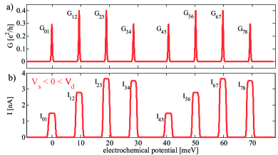
The conductance trace exhibits four-electron periodicity (Fig. 2a), with two equal in height central peaks for the transitions N=4​m+1β†’N+1𝑁4π‘š1→𝑁1N=4m+1\to N+1, N=4​m+2β†’N+1𝑁4π‘š2→𝑁1N=4m+2\to N+1, and two smaller peaks for N=4​mβ†’N+1𝑁4π‘šβ†’π‘1N=4m\to N+1, N=4​m+3β†’N+1𝑁4π‘š3→𝑁1N=4m+3\to N+1 also equal in height. The relative height between central and outer peaks is G4​m+1, 4​m+2m​a​x/G4​m,4​m+1m​a​x=27/(10+4​6)β‰ˆ1.36superscriptsubscript𝐺4π‘š14π‘š2π‘šπ‘Žπ‘₯superscriptsubscript𝐺4π‘š4π‘š1π‘šπ‘Žπ‘₯2710461.36G_{4m+1,\ 4m+2}^{max}/G_{4m,4m+1}^{max}=27/(10+4\sqrt{6})\approx 1.36, independent of the ratio Ξ³s/Ξ³dsubscript𝛾𝑠subscript𝛾𝑑\gamma_{s}/\gamma_{d}.

In the bias regime $\varepsilon_{0}\gg\left|eV_{l}\pm\Delta E\right|\gg kT$ is $\Delta f=1$. If e.g. $eV_{s}-\Delta E<0$ and $eV_{d}-\Delta E>0,$ such that tunneling is preferable rom source to drain, we find $I_{N,N+1}=eC_{N,N+1}C_{N+1,N}\gamma_{s}\gamma_{d}/(\gamma_{s}C_{N,N+1}+\gamma_{d}C_{N+1,N}).$ In this regime, the nonlinear conductance will still exhibit four-electron periodicity, Fig. 2b. For $\gamma_{s}=\gamma_{d}$ one still expects two equal central peaks and two smaller outer peaks with ratio $3/2$. If Ξ³sβ‰ Ξ³dsubscript𝛾𝑠subscript𝛾𝑑\gamma_{s}\neq\gamma_{d} this latter symmetry is lost. If we invert the sign of the bias voltage, the current is obtained by exchanging $\gamma_{s}$ with $\gamma_{d}$.

Refer to caption
Figure 2: a) Conductance vs. electrochemical potential in the linear regime $eV\ll k_{B}T\ll\varepsilon_{0}$. Despite asymmetric contacts, the two central peaks and the two outer peaks have equal height. b) Current in the regime $\varepsilon_{0}\gg\left|eV_{l}\right|\gg kT$. Asymmetry effects become visible. Four-electron periodicity is still observed. Parameters are $E_{c}=9.5$ meV; $k_{B}T=0.10$ meV, $\varepsilon_{0}=2.9$ meV, $\gamma_{s}=5\gamma_{d}=4.9\cdot 10^{10}s^{-1}$.

High bias regime. In the bias regime e​V>Ξ΅0𝑒𝑉subscriptπœ€0eV>\varepsilon_{0} states with bosonic as well as fermionic excitations contribute to transport. An analytical treatment is not possible, except to define the position of the various excitation lines. The resonance condition for tunneling in/out of lead Ε‚italic-Ε‚\l is as usually given by e​Vl+Δ​EΒ±=0𝑒subscript𝑉𝑙Δsuperscript𝐸plus-or-minus0eV_{l}+\Delta E^{\pm}=0, where Δ​EΒ±=Β±(ENΒ±1βˆ’EN).Ξ”superscript𝐸plus-or-minusplus-or-minussubscript𝐸plus-or-minus𝑁1subscript𝐸𝑁\Delta E^{\pm}=\pm\left(E_{N\pm 1}-E_{N}\right). Besides the resonance condition, also the overlap integral between initial and final state determines the rates, and hence the ”active” resonance lines contributing to the current. 
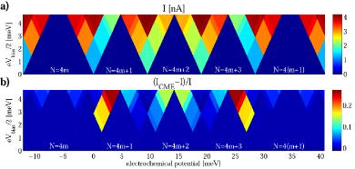
Fig 3a shows the current in a bias voltage-electrochemical potential plane for the symmetric case Ξ³s=Ξ³dsubscript𝛾𝑠subscript𝛾𝑑\gamma_{s}=\gamma_{d}. By choosing the addition energies provided in Sapmaz2005 Δ​μ1=Ec=9.5Ξ”subscriptπœ‡1subscript𝐸𝑐9.5\Delta\mu_{1}=E_{c}=9.5 meV and Δ​μ2=13.4Ξ”subscriptπœ‡213.4\Delta\mu_{2}=13.4 meV, we can reproduce all the excitation lines from sample C in Sapmaz2005 . Moreover, we find a level spacing Ξ΅0=2.9subscriptπœ€02.9\varepsilon_{0}=2.9 meV, which well agrees with the estimated length for sample C of 750750750 nm. We compare with the mean field parameters: to fit the data, an unusually large exchange interaction J=2.9𝐽2.9J=2.9 meV as well as a band shift Ξ΅0β€‹Ξ”β‰ˆJsubscriptπœ€0Δ𝐽\varepsilon_{0}\Delta\approx J had to be assumed in Sapmaz2005 (in our theory is Ξ΅0Ξ”β‰ˆJβ‰ˆ0)\varepsilon_{0}\Delta\approx J\approx 0). This yields a level spacing three times larger than the one obtained from our treatment and not consistent with the measured SWNT length.

Finally, the effect of the coherences induced by the bosonic excitations is shown in Fig. 3b, where a difference plot for the current with and without coherences is shown. Though the coherences do not qualitatively change the current, they do have a quantitative influence in a region of intermediate bias $V$. A further indication for non-Fermi liquid behavior could lie in negative differential (NDC) features originating from spin-charge separation, as predicted for a spinful Luttinger liquid quantum dot Cavaliere2004 . Asymmetric contacts are a necessary requirement. We checked these predictions as possible explanation of the NDC seen in Sapmaz2005 . We confirm that (also for non-relaxed bosons) NDC occurs. However, very large asymmetries must be assumed. Moreover, in contrast to the experiments, all the NDC lines have the same slope.

To conclude, we discussed linear and nonlinear transport in SWNT quantum dots using a bosonization approach. Our results are in quantitative agreement with experimental findings in Sapmaz2005 . Further work to explain the nature of the NDC seen in Sapmaz2005 is needed.

Refer to caption
Figure 3: a) Current in a bias voltage - electrochemical potential plane for the symmetric contacts case. b) Difference plot of the current with and without coherences. Here $k_{B}T=0.01$ meV and $\varepsilon_{0}/\varepsilon_{c+q}\approx 0.21$. Other parameters are as in Fig. 2a.

***

Useful discussions with S. Sapmaz and support by the DFG under the program GRK 638 are acknowledged.

References

  • (1) R. Saito, G. Dresselhaus, M. Dresselhaus, Physical Properties of Carbon nanotubes (Imperial College Press. London 1998).
  • (2) R. Egger and A. O. Gogolin, Phys. Rev. Lett. 79, 5082 (1997); Eur. Phys. J. B 3, 281 (1998).
  • (3) C. Kane, L. Balents and M. P. A. Fisher, Phys. Rev. Lett. 79, 5086 (1997).
  • (4) M. Bockrath et al., Nature 397, 598 (1999).
  • (5) H. W. Ch. Postma et al., Science 293, 76 (2001).
  • (6) S. J. Tans et al., Nature 386, 474 (1997).
  • (7) D. H. Cobden and J. NygΓ₯rd, Phys. Rev. Lett. 89, 046803 (2002).
  • (8) W. Liang, M. Bockrath and H. Park, Phys. Rev. Lett. 88, 126801 (2002).
  • (9) S. Sapmaz et al., Phys. Rev. B 71, 153402 (2005).
  • (10) S. Moriyama et al., Phys. Rev. Lett. 94, 186806 (2005).
  • (11) S.-H. Ke, H. U. Baranger and W. Yang, Phys. Rev. Lett. 91, 116803 (2003).
  • (12) Y. Oreg, K. Byczuk and B. I. Halperin, Phys. Rev. Lett. 85, 365 (2000).
  • (13) M. Fabrizio, A. O. Gogolin, Phys. Rev. B 51, 17827 (1995).
  • (14) In the case of noninteracting electrons and unpolarized leads, the CME is always correct if the usual Bloch wave Slater determinants are used as energy eigenstates.
  • (15) F. Cavaliere et al., Phys. Rev. Lett. 93, 036803 (2004).