Spectral formulation and WKB approximation for rare-event statistics in reaction systems

Abstract

We develop a spectral formulation and a stationary WKB approximation for calculating the probabilities of rare events (large deviations from the mean) in systems of reacting particles with infinite-range interaction, describable by a master equation. We compare the stationary WKB approximation with a recent time-dependent semiclassical approximation developed, for the same class of problems, by Elgart and Kamenev. As a benchmark we use an exactly solvable problem of the binary annihilation reaction $2A\to\emptyset$.

I Introduction

Since the pioneering works of Delbrück delb , Bartholomay barth and McQuarrie et al. McQuarrie1 ; McQuarrie , kinetics of reacting systems with infinite-range interaction, containing a large but finite number of molecules or agents (such as bacteria, cells, animals or even humans) have attracted much attention gardiner ; vankampen . While the change in time of the average number of particles in such systems may be describable by (continuum) rate equations, one often needs to know the probability of a non-typical behavior. This necessitates going beyond the rate equations, and a standard way of achieving this goal is provided by the master equation of a gain-loss type which directly deals with $P_{n_{1},n_{2},...,n_{N}}(t)$: the probability of simultaneously having $n_{1}$ particles of the first type, $n_{2}$ particles of the second type, $\dots$, and $n_{N}$ particles of the $N$th type at time $t$ gardiner ; vankampen . Though providing a complete description, the master equation is rarely solvable analytically, so various approximations are in use gardiner ; vankampen . Probably the most widely used approximation is the Fokker-Planck equation which usually suffices when one is not interested in extreme statistics, such as extinction time kamenev ; Sander . Being interested in extreme statistics, we will exploit here a well-known mathematical formulation (see, e.g. gardiner ) which, though exactly equivalent to the master equation, deals instead with a generating function $G(\mathbf{x},t)$ which encodes all the probabilities $P_{n_{1},n_{2},...,n_{N}}(t)$. The generating function is defined in the following way:

$$G(\mathbf{x},t)=\sum_{n_{1}=0,\,\dots,\,n_{N}=0}^{\infty}\left(\prod_{i=1}^{N}x_{i}^{n_{i}}\right)P_{n_{1},n_{2},...,n_{N}}(t)\,,$$ (1)

whereas the probabilities $P_{n_{1},n_{2},...,n_{N}}(t)$ are recovered by differentiation:

$$\left.P_{n_{1},\dots,n_{N}}(t)=\frac{1}{\prod_{i=1}^{N}n_{i}!}\frac{\partial^{n_{1}+\dots+n_{N}}G(\mathbf{x},t)}{\partial x_{1}^{n_{1}}\cdots\partial x_{N}^{n_{N}}}\right|_{\mathbf{x}=\mathbf{0}}\,.$$ (2)

This formulation transforms the master equation (an infinite set of differential difference equations) into a single linear partial differential equation for $G(\mathbf{x},t)$:

$$\frac{\partial G(\mathbf{x},t)}{\partial t}=\hat{L}G(\mathbf{x},t)\,,$$ (3)

where $\hat{L}$ is a real linear differential operator which involves derivatives with respect to the auxiliary variables $\mathbf{x}=(x_{1},x_{2},\dots,x_{N})$. The initial condition for this equation is supplied by Eq. (1) with the time-dependent probabilities replaced by their (prescribed) values at $t=0$. When the rate constants are time-independent, the operator $\hat{L}$ is independent of time. There is one universal boundary condition in this formulation. Indeed, as

$$\sum_{n_{1}=0,\,\dots,\,n_{N}=0}^{\infty}P_{n_{1},n_{2},...,n_{N}}(t)=1\,,$$ (4)

one immediately gets

$$G(x_{1}=1,\dots,x_{N}=1;t)=1\,.$$ (5)

Correspondingly, $\hat{L}G(\mathbf{x},t)$ must vanish at $\mathbf{x}=(x_{1},x_{2},\dots,x_{N})=(1,1,\dots,1)$.

This paper will be limited to a single species, $N=1$. In this case the generating function $G(x,t)$ is

$$G(x,t)=\sum_{n=0}^{\infty}x^{n}P_{n}(t)\,,$$ (6)

the probabilities $P_{n}(t)$ are

$$\left.P_{n}(t)=\frac{1}{n!}\frac{\partial^{n}G(x,t)}{\partial x^{n}}\right|_{x=0}\,,$$ (7)

the evolution equation for $G$ is

$$\frac{\partial G(x,t)}{\partial t}=\hat{L}G(x,t)\,,$$ (8)

and the universal boundary condition (5) is

$$G(x=1,t)=1\,.$$ (9)

The initial condition is

$$G(x,0)\equiv G_{0}(x)=\sum_{n=0}^{\infty}x^{n}P_{n}(0)\,.$$ (10)

We will be interested in the important class of problems where the operator $\hat{L}$ is of the second order secondorder . The crux of our approach is that, for any time-independent second-order linear differential operator $\hat{L}$, one can expand $G(x,t)$ in a complete set of properly constructed orthogonal spatial eigenfunctions of the operator $\hat{L}$ hermit ; Arfken . The linear ordinary differential equation for these eigenfunctions can be obtained, for any specific problem, by separation of variables. By a proper change of variables one can always eliminate the first derivative from this equation, and arrive at a spectral problem for a stationary Schrödinger equation for a zero-energy particle in a potential $V(x,\mu)$ which depends on a parameter $\mu$ coming from the separation of variables. This parameter, unknown a priori, represents the eigenvalue of this problem. This spectral formulation is exact, and it paves the way to a systematic computation of the probabilities $P_{n}(t)$, where $n$ can be significantly different from the “typical”, or average number of particles. Using the probabilities, one can accurately estimate a host of quantities of interest, for example, the average extinction time and the lifetime distribution. The present work is mainly concerned with one useful technique within the framework of the spectral formulation: the WKB approximation Landau ; orszag which yields semiclassical eigenvalues and eigenfunctions. Using these, one can construct an approximate solution of the initial value problem for $G(x,t)$ and, by virtue of Eq. (7), calculate $P_{n}(t)$ for $n\gg 1$.

As Eq. (3) is readily interpretable as a (non-Hermitian) time-dependent Schrödinger equation with imaginary time, there were earlier quantum mechanical interpretations of rare event statistics in reacting systems, such as the Doi-Peliti formalism of second quantization Doi ; Peliti ; Mattis . Still another approach to this class of problems has been recently suggested by Elgart and Kamenev kamenev . Instead of dealing with the creation and annihilation operators, as is customary in the second quantization approach, Elgart and Kamenev reformulated the time-dependent problem in semiclassical terms, employing two strong inequalities: $n\gg 1$ and $\bar{n}(t)\gg 1$, where $\bar{n}(t)$ is the average number of particles in the system at time $t$. They showed that classical dynamics corresponding to the Hamiltonian of the problem provide a valuable information about the rare-event statistics, and that this approach is greatly superior to the more customary Fokker-Planck description. Elgart and Kamenev start with the ansatz $G(x,t)=\exp[-S(x,t)]$ in Eq. (8). Then, neglecting the $\partial_{xx}S$ term, they arrive at a Hamilton-Jacobi equation for $S(x,t)$ which, for a time-independent $\hat{L}$, is solvable landaumech . This procedure yields $G(x,t)$ and, by virtue of Eq. (7), the probabilities $P_{n}(t)$. Elgart and Kamenev illustrated this approach on several pedagogical examples which included various combinations of binary annihilation, branching, decay and creation of particles.

As explained above, we suggest in this work a different type of semiclassical approximation for this non-Hermitian quantum mechanics: a stationary WKB approximation based on an exact spectral formulation. We will show that the two semiclassical approximations complement each other, each of them being advantageous in some region of the parameter space. We will demonstrate our approach by a simple example of binary annihilation reaction $2A\to^{\lambda}\hskip 5.69054pt\emptyset$, where $\lambda>0$ is the rate constant. In this case the master equation is

$$\frac{d}{dt}{P}_{n}(t)=\frac{\lambda}{2}\left[(n+2)(n+1)P_{n+2}(t)-n(n-1)P_{n}(t)\right]\,,$$ (11)

while the evolution equation for $G(x,t)$ takes the form

$$\frac{\partial G}{\partial t}=\frac{\lambda}{2}(1-x^{2})\frac{\partial^{2}G}{\partial x^{2}}\,.$$ (12)

This example is instructive for two reasons. First, it is one of the examples used by Elgart and Kamenev kamenev to illustrate their time-dependent semiclassical approach. Second, and no less important, it is exactly solvable. McQuarrie et al. McQuarrie used the exact solution to find the average number of particles and the variance versus time, when starting from a fixed even number of particles. We significantly extend the analytical solution in Appendix and find the probabilities $P_{n}(t)$ for all $n$ and $t$, and their various asymptotics. Using these findings, we also calculate the probability distribution of lifetimes of the particles in this system and the average extinction time. These exact results provide a benchmark for our WKB theory. In principle, the strong inequality $n\gg 1$ is the only criterion required in this theory for all times. We observed, however, that in practice one also needs to require $n\gtrsim\bar{n}$, in order to avoid loss of accuracy resulting from summation of many large terms of alternating sign. We will show that, in the region of $n\gtrsim\bar{n}$, the stationary WKB formalism is much more accurate than the time-dependent formalism due to Elgart and Kamenev, while in the region of $n\lesssim\bar{n}$ the time-dependent formalism (which circumvents the summation of large terms of alternating sign) is advantageous.

Here is a layout of the rest of the paper. In Section II we apply separation of variables to Eq. (12), arrive at a Sturm-Liouville eigenvalue problem and find approximate solutions to this problem by using the WKB approximation. Then we solve, in Section III, an initial value problem, compute the respective approximate probabilities $P_{n}(t)$ and compare them with the exact probabilities and their asymptotics, derived in Appendix. In Section IV we compare the predictions of the time-dependent semiclassical formulation kamenev with the exact results and establish the validity of the time-dependent and stationary semiclassical approximations. Section V presents a brief summary and discussion of our results.

II Spectral formulation and WKB approximation

II.1 Boundary conditions and steady state solution

To complete the formulation of the problem for Eq. (12), we need two boundary conditions. The first of them, Eq. (9), is universal. The second one, at $x=-1$, readily follows from Eq. (12) itself: $G(x=-1,t)=C=const$, where $C=G_{0}(x=-1)$ is determined by the initial data (10) second .

The limit of $t\to\infty$ corresponds to a steady state solution of Eq. (12): $G_{s}(x)=A+Bx$. To obey the boundary conditions at $x=\pm 1$, we choose $A=(1+C)/2$ and $B=(1-C)/2$. When $C=1$ (an even number of particles at $t=0$), the steady state solution $G_{s}(x)=1$ corresponds to an empty system: $P_{n}=\delta_{n0}$, where $\delta_{ij}$ is the Kroenecker delta. When $C=-1$ (an odd number of particles at $t=0$), one obtains $G_{s}(x)=x$. This corresponds to a single particle, $P_{n}=\delta_{n1}$, which lives forever as there are no particles it can react with.

II.2 Separation of variables and eigenvalue problem

Now let us consider the time-dependent part of the generating function: $g(x,t)=G(x,t)-G_{s}(x)$. As $g(x,t)$ must vanish at $x=\pm 1$, we can look for solutions of the equation for $g(x,t)$,

$$\frac{\partial g}{\partial t}=\frac{\lambda}{2}(1-x^{2})\frac{\partial^{2}g}{\partial x^{2}}\,,$$ (13)

in the separable form $g(x,t)=\exp(-\gamma t)\,\varphi(x)$. We obtain

$$\varphi^{\prime\prime}(x)+\frac{\mu^{2}\varphi(x)}{1-x^{2}}=0\,,$$ (14)

where $\mu^{2}=2\gamma/\lambda$, and $\varphi(\pm 1)=0$. Equation (14) can be interpreted as a stationary Schrödinger equation for a zero-energy particle ($m=\hbar=1$) in the singular potential

$$V(x)=\left\{\begin{array}[]{rcl}-\frac{\mu^{2}}{2(1-x^{2})}\,,&&|x|<1\\ +\infty\,,&&|x|\geq 1\,,\end{array}\right.$$ (15)

see Fig. 1, with (a priori unknown) magnitude $\mu^{2}$ which plays the role of eigenvalue. The problem is exactly solvable in terms of Legendre polynomials, and the solution is presented in Appendix. In the next subsection we will proceed as if we were unaware of the exact solution, and find the spectrum of $\mu$ and the eigenfunctions in the WKB approximation.

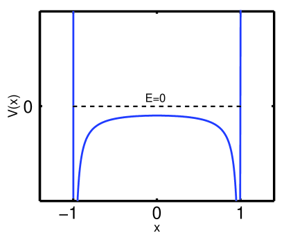
Figure 1: (Color online) Shown by the blue solid lines is the singular potential $V(x)$, given by Eq. (15). The vertical scale is arbitrary.

II.3 Stationary WKB approximation: wave functions and quantization

The crucial assumption of our semiclassical theory is that the main contribution to the probabilities $P_{n}(t)$ with $n\gg 1$ comes from the semiclassical region of spectrum of $\mu$, where $\mu\gg 1$ and the eigenfunctions have multiple zeros on the interval $|x|<1$. We will verify this assumption a posteriori. Employing the strong inequality $\mu\gg 1$, we find by a standard calculation Landau ; orszag two independent (even and odd) WKB solutions of Eq. (14):

$$\varphi_{even}(x) \simeq (1-x^{2})^{1/4}\cos(\mu\arcsin x)$$ (16)

$$\varphi_{odd}(x) \simeq (1-x^{2})^{1/4}\sin(\mu\arcsin x)\,.$$ (17)

To quantize the eigenvalue $\mu$, we must use the boundary conditions at $x=\pm 1$. The WKB solutions (16) and (17) are invalid, however, at and near the singular points $x=\pm 1$. To determine the solutions there we first solve Eq. (14) in a small vicinity of each of these points. Here it suffices to consider the point $x=1$. Let us introduce a new coordinate $\xi=1-x\ll{1}$ and neglect the subleading terms in the expansion of the potential $V(x)$ near $x=1$. Equation (14) becomes

$$2\xi\varphi^{\prime\prime}(\xi)+\mu^{2}\varphi(\xi)=0\,.$$ (18)

The two independent solutions are

$$\varphi_{1}(\xi)=\xi^{1/2}J_{1}[\mu(2\xi)^{1/2}]$$ (19)

and

$$\varphi_{2}(\xi)=\xi^{1/2}Y_{1}[\mu(2\xi)^{1/2}]\,,$$ (20)

where $J_{1}$ and $Y_{1}$ are the Bessel functions of the first and second kind, respectively. Only $\varphi_{1}(\xi)$ obeys the required boundary condition $\varphi(\xi=0)=0$, so $\varphi_{2}(\xi)$ must be discarded. Now we can match $\varphi_{1}(\xi)$ with each of the WKB solutions (16) and (17). Indeed, when $\mu\gg 1$, the solution $\varphi_{1}(\xi)$ remains valid at $\mu\xi^{1/2}\gg 1$, as long as $\xi\ll 1$. It has, therefore, a common region of validity with the WKB solutions. We use the asymptotic expansion bateman

$$J_{1}(z)\simeq\sqrt{\frac{2}{\pi{z}}}\,\cos\left(\frac{3\pi}{4}-z\right)\;\;\;\mbox{at}\;\;\;z\gg{1}$$ (21)

and obtain, up to a constant factor,

$$\varphi_{1}(\xi) \simeq \xi^{1/4}\sin\left(\mu\sqrt{2\xi}-\frac{\pi}{4}\right)$$ (22)

$$= (1-x)^{1/4}\sin\left[\mu\sqrt{2(1-x)}-\frac{\pi}{4}\right]\,.$$

Now we expand the even WKB solution (16) at $1-x\ll{1}$:

$$\varphi_{ev}(x)\simeq(1-x)^{1/4}\sin\left[\mu\sqrt{2(1-x)}-\frac{\mu\pi}{2}-\frac{\pi}{2}\right]\,.$$ (23)

Matching the asymptotes (22) and (23), we obtain the discrete spectrum eigenvalues corresponding to the even eigenfunctions:

$$\mu=2k-\frac{1}{2}\,,$$ (24)

where $k\gg 1$ is an integer. In a similar way we obtain the discrete spectrum for the odd eigenfunctions:

$$\mu=2k+\frac{1}{2}\,.$$ (25)

The eigenvalues (24) and (25) coincide, in the leading and subleading orders in $k\gg{1}$, with the exact eigenvalues $(4k^{2}-2k)^{1/2}$ and $(4k^{2}+2k)^{1/2}$, respectively, see Appendix. Furthermore, the corresponding WKB eigenfunctions provide an accurate approximation, see Fig. 2, to the exact eigenfunctions [which are orthogonal, with respect to the inner product with the weight function $w(x)=(1-x^{2})^{-1}$, on the interval $|x|<1$, and form a complete set]. We normalize the approximate eigenfunctions $u_{l}(x)$ by demanding

$$\int_{-1}^{1}u_{l}^{2}(x)w(x)\,dx=1\,.$$ (26)

The normalized even WKB eigenfunctions are

$$u_{2k}(x)=\left\{\begin{array}[]{ll}u_{2k}^{(a)}(x)&=(-1)^{k}\sqrt{\frac{2}{\pi}}(1-x^{2})^{1/4}\\ &\times\cos\left[\mu_{k}\arcsin x\right]\\ &\;\;\;\;\;\;\;\mbox{for}\;0\leq|x|<1-\varepsilon\,,\\ u_{2k}^{(b)}(x)&=-\sqrt{2\mu_{k}(1-|x|)}\\ &\times J_{1}\left[\mu_{k}\sqrt{2(1-|x|)}\right]\\ &\;\;\;\;\;\;\;\mbox{for}\;1-\varepsilon<|x|\leq{1}\,,\end{array}\right.$$

where $1/k^{2}\ll\varepsilon\ll{1}$, $\mu_{k}=2k-1/2$, and $k\gg{1}$. For $1/\mu_{k}^{2}\ll 1-|x|\ll{1}$ the function $u_{2k}^{(a)}(x)$ coincides, in the leading order, with $u_{2k}^{(b)}(x)$. It is sufficient to use only the $u_{2k}^{a}(x)$ asymptotes in the normalization integral (26).

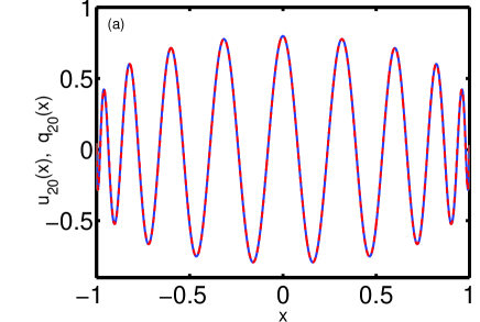
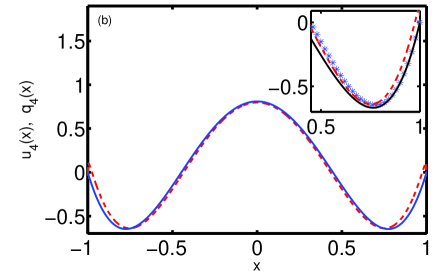
Figure 2: (Color online) The normalized WKB eigenfunctions (II.3) (the red dashed lines) and the normalized exact eigenfunctions (the blue solid lines) for $k=10$ (a) and $k=2$ (b). As one can see, a good agreement is observed even for $k=2$, while for $k=10$ the agreement is excellent. The inset in (b) shows a close vicinity of $x=1$. One can see that the function $u_{20}^{(a)}(x)$ (the red dashed line) deviates from the exact solution (indicated by the crosses) in the vicinity of $x=1$, whereas the function $u_{20}^{(b)}(x)$ (the solid line) is in excellent agreement with the exact solution there.

III Initial value problem and calculation of the probabilities

Putting everything together, we can write the WKB solution of the initial value problem for Eq. (12) as

$$G(x,t)\simeq G_{s}(x)+\sum_{l>0}a_{l}\exp\left(-\frac{\mu_{l}^{2}\lambda t}{2}\right)\,u_{l}(x)\,,$$ (27)

where each constant $a_{l}$ is equal to the inner product [with the weight function $w(x)=(1-x^{2})^{-1}$] of the respective normalized eigenfunction $u_{l}(x)$ and the function $G_{0}(x)-G_{s}(x)$. One can see that the populations of the eigenstates with $l>0$ of this non-Hermitian “quantum mechanics” are decaying exponentially in time.

Assume, for concreteness, that the initial number of particles is fixed and equal to $n_{0}=2k_{0}\gg{1}$, where $k_{0}$ is integer. In this case [see Eq. (10)] $G_{0}(x)=x^{2k_{0}}$, and one only needs the even eigenfunctions (II.3). Now we can use the orthonormality relation (26) and compute the coefficients $a_{k}$. After a lengthy algebra we obtain

$$a_{k}\simeq\frac{2}{\sqrt{\mu_{k}}}\,e^{-\frac{k(2k-1)}{2k_{0}}}\,,$$ (28)

where we have assumed $k\lesssim\sqrt{k_{0}}\ll k_{0}$, as justified below. In the leading order in $1/k\ll 1$ Eq. (28) coincides with the corresponding asymptotics (A4) of the exact result. Now Eq. (27) becomes

$$G(x,t)\simeq 1+\sum_{k=1}^{\infty}\frac{2}{\sqrt{\mu_{k}}}\,e^{\frac{-k(2k-1)}{\bar{N}(t)}}u_{2k}(x)\,,$$ (29)

where

$$\bar{N}(t)\equiv\frac{2k_{0}}{1+2k_{0}\lambda t}$$

is the average number of particles at time $t$ according to the mean-field theory. Though the sum in Eq. (29) formally runs to infinity, the dominant contribution comes from terms with $k\lesssim\sqrt{k_{0}}\ll k_{0}$, while the rest of terms give only exponentially small corrections.

To recover $P_{n}(t)$, for $1\ll n\lesssim\sqrt{k_{0}}$, we use Eq. (7):

$$P_{n}(t)\simeq\frac{1}{n!}\sum_{k=1}^{\infty}\frac{2}{\sqrt{\mu_{k}}}\left.\,e^{\frac{-k(2k-1)}{\bar{N}(t)}}\;\frac{\partial^{n}u_{2k}(x)}{\partial\,x^{n}}\right|_{x=0}.$$ (30)

As our WKB approximation assumes $\mu_{k}=2k-1/2\gg 1$, the first few terms of the sum in Eq. (30) may seem inaccurate. It turns out, however, that the sum actually starts from $k=n/2$, see below. Therefore, at $1\ll n\lesssim\sqrt{k_{0}}$ all the terms of the sum in Eq. (30) are accurate.

Equation (30) is the central result of the stationary WKB approximation for the binary annihilation problem. To compute the $n$-th derivative of the WKB eigenfunctions $u_{2k}(x)$, entering Eq. (30), we can analytically continue $u_{2k}(x)$ into the complex plane. By virtue of the Cauchy theorem

$$I\equiv\frac{1}{n!}\left.\frac{\partial^{n}u_{2k}(x)}{\partial\,x^{n}}\right|_{x=0}=\frac{1}{2\pi i}\oint_{C}\frac{u_{2k}(z)dz}{z^{n+1}}\,,$$ (31)

where the integration is performed over a closed contour $C$ in the complex $z$-plane around the pole $x=0$ inside the region of analyticity of $u_{2k}(x)$. We can put here $u_{2k}(z)=u_{2k}^{(a)}(z)$, since the main contribution to the integral, as shown below, comes from the region far from the points $x=\pm 1$, in the vicinity of which $u_{2k}^{(a)}(z)$ is inaccurate. We obtain

$$I=\frac{(-1)^{k}}{\sqrt{2}\pi^{3/2}i}\,\mbox{Im}\left[\oint_{C}g(z)\,e^{(n-1)f(z)}dz\right]\,,$$ (32)

where $f(z)=iA\arcsin(z)-\ln(z)$, $g(z)=\frac{(1-z^{2})^{1/4}}{z^{2}}$ and $A=\mu_{k}/(n-1)$. As $n\gg 1$, the integral in (32) can be evaluated using the saddle point approximation orszag . This is done by deforming the contour $C$, so that it passes through the saddle point $z_{*}=x_{*}+iy_{*}$, where $u(x,y)=\mbox{Re}[f(z)]$ obtains its maximum, and consequently $v(x,y)=\mbox{Im}[f(z)]$ is constant. By choosing the contour at the saddle point to be parallel to the direction of the steepest descent of $u(x,y)$, we can replace the integration over the complex plane by integration over the real axis, having to multiply the result by a constant phase: the value of $v(x,y)$ at the saddle point. The saddle point can be found from the equation $f^{\prime}(z)=0$. For $k<n/2$ (that is, $A<1$), the saddle point lies on the real axis: $z_{*}^{(1)}=[1-A^{2}]^{-1/2}$, whereas for $k\geq{n/2}$ (that is, $A>1$) it lies on the imaginary axis: $z_{*}^{(2)}=-i[A^{2}-1]^{-1/2}$. In each of these cases Eq. (32) becomes orszag

$$I=\frac{(-1)^{k}}{\sqrt{2}\pi^{3/2}i}\,\mbox{Im}\left[\frac{\sqrt{2\pi}g(z_{*})e^{(n-1)f(z_{*})}e^{i\alpha}}{\sqrt{(n-1)|f^{\prime\prime}(z_{*})|}}\right]\,,$$ (33)

where $\alpha$ is the angle of the contour with respect to the positive real axis at the saddle point, where the contour is chosen to be parallel to $-\nabla u(x,y)$.

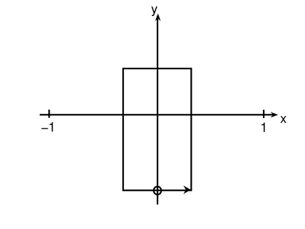
Figure 3: A possible contour $C$, see Eq. (32). The direction of the contour in the vicinity of the saddle point $z=z_{*}^{(2)}$ (marked by the circle) is chosen to be along $-\nabla u(x,y)$ at $z_{*}^{(2)}$, implying in this case $\alpha=0$. As $n\gg{1}$, the contribution of the rest of the contour (as long as it encircles $z=0$) is exponentially small.

This procedure yields markedly different results in the cases of $A<1$ ($k<n/2$) and $A>1$ ($k\geq n/2$). For $A<1$, upon substituting $z_{*}^{(1)}$ and deforming the contour so that $\alpha=\pi/2$ in its vicinity, we realize that the result inside the brackets in Eq. (33) is real which yields $I=0$. Therefore, the saddle-point asymptote Eq. (33) predicts that the $n$-th derivative of the eigenfunctions $u_{2k}(x)$ vanishes for $k<n/2$, so the sum in Eq. (30) starts from $k=n/2$. This could be expected, as the same kind of behavior is exhibited by the exact eigenfunctions $q_{2k}(x)$, which are polynomials of order $2k$, see Appendix.

After some algebra, Eq. (33) yields, for $k\geq n/2$

$$I\simeq\frac{(-1)^{k-n/2}e^{1/4}k^{3/2}2^{n}\left(k+\frac{n}{2}\right)^{k+\frac{n}{2}-1}}{\pi\,n^{n+\frac{1}{2}}\,\left(k-\frac{n}{2}+\frac{1}{4}\right)^{k-\frac{n}{2}+\frac{1}{2}}}\,,$$ (34)

where we have substituted $z_{*}^{(2)}$ for the saddle point. A possible contour $C$ is shown in Fig. 3. We can see now that, as the saddle point $z_{*}$ lies on the imaginary axis, the contour does not have to come close to $x=\pm{1}$, thus justifying the use of $u_{2k}^{(a)}(z)$ for $u_{2k}(z)$. The saddle point approximation is only valid when $|f^{\prime\prime\prime}(z_{*})|/|f^{\prime\prime}(z_{*})|^{3/2}\ll\sqrt{n}$ orszag . For $k\geq{n/2}$ this requirement is equivalent to $k-n/2\gg 1$. We will see shortly, however, that the results remain quite accurate even for $k-n/2={\cal O}(1)$. Now we can rewrite Eq. (30) as

$$P_{n}(t) \simeq \frac{e^{1/4}2^{n+\frac{1}{2}}}{\pi\,n^{n+\frac{1}{2}}}\sum_{k=\frac{n}{2}}^{\infty}\frac{(-1)^{k-\frac{n}{2}}\,k\left(k+\frac{n}{2}\right)^{k+\frac{n}{2}-1}}{\left(k-\frac{n}{2}+\frac{1}{4}\right)^{k-\frac{n}{2}+\frac{1}{2}}}$$ (35)

$$\times \,e^{\frac{-k(2k-1)}{\bar{N}(t)}}.$$

We immediately notice that this formula is very similar to Eq. (A12). Moreover, the two expressions coincide if we rewrite the factor $(k-n/2)^{k-n/2+1/2}$ in the denominator of Eq. (A12) as $(k-n/2+1/4-1/4)^{k-n/2+1/2}$, assume $k-n/2\gg 1$ and use the asymptote $(1+\xi/u)^{u}\simeq e^{\xi}$ at $u\gg 1$. As Eq. (A12) gives an accurate approximation to the exact probabilities at $n\sim\bar{N}$ (see Appendix), the same is true for the stationary WKB result (A12). For $n\gg\bar{N}$ it suffices to take into account only the first term, $k=n/2$ in the sum of Eq. (35) which yields

$$P_{n}(t)\simeq\frac{2^{n+\frac{1}{2}}\,e^{\frac{1}{4}}}{\pi\sqrt{n}}\,e^{\frac{-n(n-1)}{2\bar{N}(t)}}\,.$$ (36)

This asymptote coincides, up to a factor $\sqrt{2/\pi}\,e^{1/4}\simeq{0.976}$, with Eq. (A11) that gives an accurate approximation to the exact probabilities in this limit, see Appendix. Therefore, in the region of $n\gtrsim\bar{N}$ the stationary WKB theory is accurate, as can be seen from Figures 4-6. Importantly, the asymptote (36) does not demand $\bar{N}\gg 1$ and therefore remains valid at long times, $\lambda t\gtrsim 1$, when the average number of particles is already small, see Fig. 7.

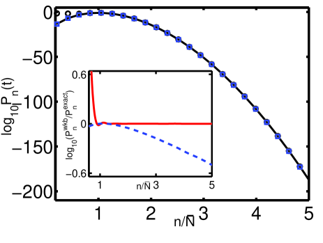
Figure 4: (Color online) The decimal logarithm of $P_{n}(t)$ as a function of $n/\bar{N}$ for $\lambda{t}=0.02$ and $n_{0}=10^{3}$. Shown are the exact probabilities (A7) (the solid line), the stationary WKB probabilities (30) (the empty circles) and the time-dependent WKB probabilities (40) (the blue squares). Inset shows the logarithm of the ratio of the stationary WKB probabilities and the exact ones (the red solid line), and the logarithm of the ratio of the time-dependent WKB probabilities and the exact ones (the blue dashed line), versus $n/\bar{N}$. As $n/\bar{N}$ grows, the time-dependent WKB solution deteriorates, whereas when $n$ goes down below $\bar{N}$, the stationary WKB solution deteriorates.

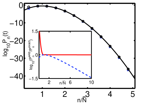
Figure 5: Same as in Fig. 4, but for $\lambda{t}=0.1$.

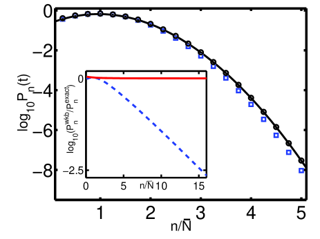
Figure 6: Same as in Fig. 4, but for $\lambda{t}=0.5$. One can clearly see that the time-dependent WKB result is already inaccurate at $n\gtrsim\bar{N}$, while the stationary WKB result keeps its high accuracy there.

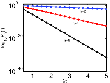
Figure 7: Long time asymptotics of $P_{n}(t)$. Shown is the decimal logarithm of $P_{n}(t)$ as a function of $\lambda t$ for $n_{0}=10^{3}$ and $n=2,4,$ and $6$. The circles denote the stationary WKB solution [Eq. (36)], the solid lines denote the exact solution [Eq. (A7)]. Notice excellent agreement even for small $n$.

IV Time-dependent semiclassical solution versus exact solution

The time-dependent semiclassical approximation, suggested by Elgart and Kamenev kamenev , differs from the stationary WKB approximation in that it deals semiclassically with the original non-Hermitian Schrödinger equation (8) (a partial differential equation), rather than with the set of ordinary differential equations obtained by the separation of variables in Eq. (8). Using the ansatz $G(x,t)=\exp[-S(x,t)]$ and neglecting the $\partial_{xx}S$ term, one arrives at a Hamilton-Jacobi equation. For the binary annihilation problem this equation is kamenev

$$\frac{\partial{S}}{\partial{t}}=\frac{\lambda}{2}(x^{2}-1)\left(\frac{\partial{S}}{\partial{x}}\right)^{2}\,.$$ (37)

Elgart and Kamenev kamenev found an exact solution to this equation:

$$S(x,t)=\frac{1}{2}\,\bar{N}(t)\arccos^{2}x\,.$$

The respective generating function

$$G(x,t)=\exp\left[-\frac{1}{2}\,\bar{N}(t)\arccos^{2}x\right]$$ (38)

obeys the boundary condition (9) exactly, and the initial condition $G(x,t=0)=x^{n_{0}}$ with a high accuracy as long as $n_{0}\gg 1$. The probabilities $P_{n}(t)$ can be calculated from the equation

$$\left.P_{n}(t)=\frac{1}{n!}\frac{\partial^{n}G(x,t)}{\partial x^{n}}\right|_{x=0}\,=\frac{1}{2\pi{i}}\oint\frac{dz}{z^{1+n}}G(z,t)\,,$$ (39)

where the integration is performed over a closed contour including $z=0$ in the complex $z$ plane, inside the region of analyticity of $G(z,t)$. For $n\gg{1}$ and $\bar{N}(t)\gg 1$, the integral can be evaluated by the saddle point approximation, and the result is

$$P_{n}(t)\simeq\sqrt{\frac{1-x_{s}^{2}}{2\pi\left[n-\bar{N}(t)x_{s}^{2}\right]}}\,e^{-\bar{N}(t)\left(\frac{1}{2}\arccos^{2}x_{s}+\frac{n}{\bar{N}(t)}\ln x_{s}\right)},$$ (40)

where $x_{s}=x_{s}(n/\bar{N})$ is the root of the saddle-point equation $x_{s}(1-x_{s}^{2})^{-1/2}\arccos x_{s}=n/\bar{N}$ kamenev . For $n\ll\bar{N}(t)$ one obtains $x_{s}\simeq 2n/(\pi\bar{N})$, so

$$\ln P_{n}(t)\simeq n\ln\frac{\pi\bar{N}(t)}{2n}-\frac{\pi^{2}\bar{N}(t)}{8}+n$$ (41)

(in the corresponding asymptote of Ref. kamenev the term $n$ is missing.)

For $n\simeq\bar{N}(t)$, $x_{s}\simeq 1-(3/2)(1-n/\bar{N})$, so

$$\ln P_{n}(t)\simeq-\frac{3[n-\bar{N}(t)]^{2}}{4\bar{N}(t)}\,.$$ (42)

Finally, for $n\gg\bar{N}(t)$, $x_{s}\simeq(1/2)\,e^{n/\bar{N}}$, so

$$\ln P_{n}(t)\simeq n\ln 2-\frac{n^{2}}{2\bar{N}(t)}\,.$$ (43)

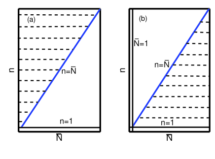
Figure 8: The dashed regions schematically show the validity of each of the two semiclassical theories on the parameter plane $(\bar{N},n)$. Figure a shows the validity domain $n\gtrsim\bar{N}$ and $n\gg 1$ of the stationary WKB theory. An additional condition for its validity is $n\lesssim\sqrt{k_{0}}\ll k_{0}$ (not shown). Figure b shows the validity domain $1\ll n\lesssim\bar{N}$ of the time-dependent WKB theory.

What are the applicability conditions of the time-dependent semiclassical approximation? The above calculations required $n_{0}=2k_{0}\gg 1$, $n\gg 1$ and $\bar{N}\gg 1$. To find out whether there is an additional condition, let us consider the $n\gg\bar{N}(t)$ asymptote of the exact result [Eq. (A11)]:

$$\ln P_{n}(t)\simeq n\ln 2-\frac{n^{2}}{2\bar{N}(t)}+\frac{n}{2\bar{N}(t)}\,.$$ (44)

A comparison of Eqs. (43) and (44) shows that the time-dependent WKB probability $P_{n}(t)$ lacks a large term $n/[2\bar{N}(t)]$ in the exponent, and therefore it greatly underestimates rare events with $n\gg\bar{N}(t)$. This effect can been seen in Figs. 4-6. On the other hand, in the region $n\lesssim\bar{N}(t)$, the time-dependent WKB theory yields a good approximation to the exact result, as it circumvents the summation of large terms of alternating sign.

Therefore, based on the analytical and numerical comparisons, we conclude that the time-dependent semiclassical approximation is accurate at $1\ll n\lesssim\bar{N}$. This obviously implies $\bar{N}\gg 1$, that is not too long times: $\lambda t\ll 1$. The stationary WKB approximation is accurate for $n\gtrsim\bar{N}$ for any $\bar{N}$, that is for all times. These results are illustrated in Figs. 4-6 which show $P_{n}(t)$ versus $n/\bar{N}$: the exact result (A7) and the predictions of each of the two approximations, Eq. (30) and Eq. (40). The validity domains of each of the two semiclassical approximations in the parameter plane ($\bar{N},n$) are shown in Fig. 8.

V Summary and Discussion

We developed a spectral formulation and a stationary WKB approximation for calculating the probabilities of rare events in systems of reacting particles with infinite-range interaction which are describable by a master equation. We extended the exact analytical solution of the binary annihilation problem $2A\to\emptyset$ and used is as a benchmark for testing the stationary WKB approximation and a recent time-dependent WKB approximation due to Elgart and Kamenev kamenev . In theory the stationary WKB approximation is always more accurate than a time-dependent WKB approximation. In practice this advantage is indeed realized in the regimes where the superposition of the different “quantum states” of the system is dominated by a small number of terms. On the contrary, when many “quantum states” are involved, virtually any approximation to the “wave functions” of individual states may alter the precise destructive interference between the different states and cause large errors. In such cases the time-dependent WKB approximation kamenev , which effectively sums over the “quantum states” without dealing with them explicitly, can be advantageous.

WKB approximation alone is insufficient for calculating the life-time probability distribution of systems which exhibit extinction. This quantity is encoded in $P_{0}(t)\equiv G(x=0,t)$ which involves a sum over all “quantum states”, including the lowest ones (see the final part of Appendix). Still, the spectral formulation can be very useful here: it clearly identifies the lowest states and provides a proper framework for calculating their eigenvalues and eigenfunctions: for example, by a variational method.

This work dealt with the case when the operator $\hat{L}$ is of the second order, and the standard machinery of Sturm-Liouville theory is therefore available. The spectral formulation itself, however, is equally applicable to higher-order operators. Furthermore, it is well known that “WKB analysis is not sensitive to the order of a differential equation” (Ref. orszag , p. 496) which paves the way to generalizations of the theory to more complicated reaction kinetics.

Finally, we have restricted ourselves in this paper to a single species. The generating function formalism, however, is applicable to any number of species [see Eqs. (1)-(5)]. Already for two species some qualitative changes are possible. Indeed, for two species, the underlying classical phase space, described by the Hamiltonian of the problem, is four-dimensional. If energy is the only integral of motion, the classical motion is non-separable and, in general, chaotic gutzwiller . Therefore, for highly-excited states, where classical mechanics and stationary WKB approximation are relevant, the spectral formulation may bring about an extension of quantum chaos to these non-Hermitian “quantum” systems.

Appendix

Here we briefly review and extend the exact solution of the binary annihilation problem, obtained by McQuarrie et al. McQuarrie . Let the initial state correspond to a fixed and even number of particles, so one only needs the even eigenfunctions of Eq. (14), with the boundary conditions $\phi(x=\pm{1})=0$. The exact even eigenfunctions are Abramowitz

$$\phi_{2k}(x)={\cal P}_{2k}(x)-{\cal P}_{2k-2}(x)\,,\;\;\;\;k=1,2,\dots\,,$$

where ${\cal P}_{l}(x)$ is the Legendre polynomial of order $l$. The corresponding exact eigenvalues are $\mu=(4k^{2}-2k)^{1/2}$. The normalized even eigenfunctions, see Eq. (26), are

$$q_{2k}(x)=\sqrt{\frac{k(2k-1)}{4k-1}}\left[{\cal P}_{2k}(x)-{\cal P}_{2k-2}(x)\right]\,.$$

The exact solution of an initial value problem for $G(x,t)$ can be written as

$$G(x,t)=1+\sum_{k=1}^{\infty}A_{k}q_{2k}(x)e^{-k(2k-1)\lambda t}\,,$$ (A1)

where the coefficients $A_{k}$ are determined by the initial data $G_{0}(x)$. For the initial data we are interested in $n_{0}=2k_{0}$, where $k_{0}=0,1,2,...$, therefore, $G_{0}(x)=x^{2k_{0}}$. Using the orthogonality relations of the Legendre polynomials, we obtain, after some algebra,

$$A_{k}=\sqrt{\frac{4k-1}{k(2k-1)}}\;\frac{\Gamma(1+k_{0})\Gamma\left(\frac{1}{2}+k_{0}\right)}{\Gamma\left(\frac{1}{2}+k_{0}+k\right)\Gamma(k_{0}-k+1)}\,,$$ (A2)

where $\Gamma(\cdot\cdot\cdot)$ is the gamma function. Owing to the presence of factor $\Gamma(k_{0}-k+1)$ in the denominator, $A_{k}$ vanishes for $k>k_{0}$. Therefore, the sum in Eq. (A1) is finite in this case, and it ends at $k=k_{0}$. The average number of particles at time $t$, $\bar{n}(t)$, can be found from the following relation:

$$\bar{n}(t)=\sum_{n=0}^{\infty}nP_{n}(t)=\left.\frac{\partial G(x,t)}{\partial x}\right|_{x=1}\,.$$

Using Eq. (A1), we obtain

$$\bar{n}(t)=\sum_{k=1}^{k_{0}}\sqrt{k(2k-1)(4k-1)}\,A_{k}\,e^{-k(2k-1)\lambda t}\,.$$ (A3)

Equations (A1)-(A3) coincide, up to notation, with the results of McQuarrie et. al. McQuarrie [they also calculated the second moment $\bar{n^{2}}(t)$]. We now extend the exact theory in three directions. First, we obtain some useful approximations for a large number of particles. Second, we calculate the probabilities $P_{n}(t)$ and their approximate asymptotics in different regimes. We use these approximations while comparing the exact solution (i) with our stationary WKB results, and (ii) with the time-dependent semiclassical approximation of Elgart and Kamenev kamenev . Third, we find the probability distribution of lifetimes of the particles in this system, and the average extinction time.

When $k\lesssim\sqrt{k_{0}}$ (see below), we can reduce Eq. (A2) to

$$A_{k}\simeq\sqrt{\frac{4k-1}{k(2k-1)}}\,e^{-\frac{k}{2k_{0}}(2k-1)}\,$$ (A4)

which yields the following approximation for $G(x,t)$:

$$G(x,t)\simeq{1}+\sum_{k=1}^{k_{0}}\sqrt{\frac{4k-1}{k(2k-1)}}\,q_{2k}(x)\,e^{-\frac{k(2k-1)}{\bar{N}(t)}}\,.$$ (A5)

Here

$$\bar{N}(t)\equiv\frac{2k_{0}}{1+2k_{0}\lambda t}\,,$$

which is the mean-field result for the average number of particles. Equation (A5) is valid for all times, as the dominant contribution to the sum comes from terms with $k\lesssim\sqrt{k_{0}}\ll k_{0}$, while the rest of terms give only exponentially small corrections. The average number of particles (A3) can be approximated as

$$\bar{n}(t)\simeq\sum_{k=1}^{k_{0}}(4k-1)\,e^{-\frac{k(2k-1)}{\bar{N}(t)}}\,.$$ (A6)

For short times, $\lambda t\ll 1$, $\bar{N}(t)\gg 1$, so the summation in Eq. (A6) can be replaced by integration. Moving the upper limit to infinity (which only causes an exponentially small error), we obtain

$$\bar{n}(t)\simeq\int_{1}^{\infty}(4k-1)\,e^{-\frac{k(2k-1)}{\bar{N}(t)}}\,dk\simeq\bar{N}(t)\,,$$

the mean-field result. In the long-time limit $\lambda t\gg 1$, $\bar{N}(t)\simeq(\lambda t)^{-1}\ll 1$, the term $k=1$ in Eq. (A6) is dominant, and we obtain $\bar{n}(t)\simeq 3\,e^{-\lambda t}$.

Now we employ Eq. (7) of the main part of the paper to calculate the probabilities $P_{n}(t)$. After some algebra we obtain the exact result:

$$P_{n}(t)=\delta_{0n}+\frac{2^{n-1}}{n!}\sum_{k=r}^{k_{0}}C_{e}(k,n)e^{-k(2k-1)\lambda t}\,,$$ (A7)

where $n$ is assumed to be even, $r=\mbox{max}(1,n/2)$, and

$$C_{e}(k,n)={A_{k}}\left[\frac{(-1)^{k-\frac{n}{2}}(4k-1)\Gamma[k-\frac{1}{2}+\frac{n}{2}]}{\sqrt{\pi}\left(k-\frac{n}{2}\right)!}\right]\,.$$ (A8)

At $n>0$ the sum in Eq. (A7) starts from $k=n/2$. This is because the eigenfunctions $q_{2k}(x)$ are polynomials of order $2k$, so the $n$-th derivative of $q_{2k}(x)$ vanish at $n>2k$.

Going to the limit of $n\gg 1$ and $k\lesssim\sqrt{k_{0}}$, and using the approximation (A4) for $A_{k}$, we can rewrite $C_{e}(k,n)$ as

$$C_{e}(k,n)\simeq\frac{(-1)^{k-\frac{n}{2}}2^{5/2}k\left(k+\frac{n}{2}\right)^{k+\frac{n}{2}-1}}{\left(k-\frac{n}{2}\right)!\,e^{k+\frac{n}{2}}}\,e^{-\frac{k(2k-1)}{2k_{0}}}\,.$$ (A9)

Therefore, at $1\ll n\lesssim\sqrt{k_{0}}$, $P_{n}(t)$ becomes

$$P_{n}(t)\simeq\frac{2^{n+1}}{n^{n+\frac{1}{2}}}\sum_{k=\frac{n}{2}}^{k_{0}}\frac{(-1)^{k-\frac{n}{2}}k\left(k+\frac{n}{2}\right)^{k+\frac{n}{2}-1}}{\sqrt{\pi}\left(k-\frac{n}{2}\right)!\,e^{k-\frac{n}{2}}}\,e^{\frac{-k(2k-1)}{\bar{N}(t)}}\,.$$

(A10)

This expression can be simplified drastically for $n\gg\bar{N}(t)$. Here the sum can be accurately approximated by its first term $k=n/2$, and we obtain

$$P_{n}(t)\simeq\frac{2^{n}}{\sqrt{\pi{n}}}\,e^{\frac{-n(n-1)}{2\bar{N}(t)}}\,.$$ (A11)

This asymptote coincides, in the limit of $1\ll n\lesssim\sqrt{k_{0}}$, with the first term of the sum in the exact result (A7).

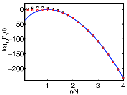
Figure 9: The exact probabilities (A7) (the solid line), the approximate probabilities (A10) (the circles), and their asymptotics (A12) and (A11) (the squares), for $n_{0}=10^{4}$ and $\bar{N}(t=0.01)\simeq 99.5$. The agreement is good for $n\gtrsim\bar{N}(t)$.

In the cases of $n\ll\bar{N}(t)$ and $n\sim\bar{N}(t)$ the leading contribution to the sum in Eq. (A10) comes from terms for which $k-n/2\gg 1$ which makes it possible to use the Stirling formula for the factor $\left(k-n/2\right)!\,$ and arrive at

$$P_{n}(t)\simeq\frac{2^{n+\frac{1}{2}}}{n^{n+\frac{1}{2}}}\sum_{k>\frac{n}{2}}^{k_{0}}\frac{(-1)^{k-\frac{n}{2}}k\left(k+\frac{n}{2}\right)^{k+\frac{n}{2}-1}}{\pi\left(k-\frac{n}{2}\right)^{k-\frac{n}{2}+\frac{1}{2}}}\,e^{\frac{-k(2k-1)}{\bar{N}(t)}}.$$

(A12)

Now let us go back to Eq. (A10). According to our analysis, it should be accurate for $1\ll n\lesssim\sqrt{k_{0}}$. A numerical comparison with the exact result (A7) [see Fig. 9] shows, however, that Eq. (A10) is accurate only at $\bar{N}\lesssim n\lesssim\sqrt{k_{0}}$. At $n\lesssim\bar{N}$ the agreement rapidly deteriorates. The disagreement stems from the fact that the sum in Eq. (A7) consists of terms of alternating sign. In the region of $n\lesssim\bar{N}$, $P_{n}(t)$ is much smaller than each of the relevant terms of the sum, while the magnitudes of the successive terms are close to each other. One can say that there is strong destructive interference of “quantum states” of the system. In this situation, virtually any approximation made in calculating the individual terms of the sum may alter the precise balance between the terms and cause large errors in the region of $n\lesssim\bar{N}$. The same problem appears in our stationary WKB theory, see Section III, which makes the time-dependent WKB approximation advantageous in this case.

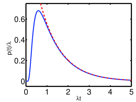
Figure 10: (Color online) The lifetime probability distribution $p(t)$ normalized to $\lambda$, as described by Eq. (A14) (the blue solid line), and its long time asymptote $p(t)/\lambda=(3/2)\,e^{-\lambda t}$ (the red dashed line).

Now we proceed to calculating the probability distribution of lifetimes of the particles, and the average extinction time. The quantity $P_{0}(t)$ is the probability of extinction at time $t$. Therefore, the lifetime probability distribution is $p(t)=dP_{0}(t)/dt$. On the other hand, $P_{0}(t)=G(x=0,t)$. Therefore, using Eq. (A1), we obtain the exact result

$$p(t)=\lambda\sum_{k=1}^{k_{0}}k(1-2k)\,A_{k}q_{2k}(0)e^{-k(2k-1)\lambda t}\,.$$ (A13)

Both $p(t)$ and all its derivatives with respect to $t$ vanish at $t=0$, so $p(t)$ is exponentially small at $\lambda t\ll 1$. When $k_{0}\gg 1$ and $\lambda t\gtrsim 1/\sqrt{k_{0}}$, Eq. (A13) can be approximated as

$$p(t)\simeq\lambda\sum_{k=1}^{\infty}k(2k-1)\,\left[{\cal P}_{2k-2}(0)-{\cal P}_{2k}(0)\right]e^{-k(2k-1)\lambda t}\,,$$ (A14)

which is independent of $k_{0}$. This universal distribution is shown in Fig. 10. The long-time tail of the distribution, $\lambda t\gtrsim 1$, is described by the first term of the sum in Eq. (A14), which yields $p(t)\simeq(3\lambda/2)\,e^{-\lambda t}$.

The average extinction time is

$$\bar{\tau} = \int_{0}^{\infty}tp(t)\,dt=\int_{0}^{\infty}\left[1-P_{0}(t)\right]\,dt=$$ (A15)

$$= \int_{0}^{\infty}\left[1-G(x=0,t)\right]\,dt\,,$$

which yields

$$\bar{\tau}=\frac{1}{\lambda}\,\sum_{k=1}^{k_{0}}\frac{A_{k}q_{2k}(0)}{k(2k-1)}\,.$$ (A16)

When $k_{0}\gg 1$, we obtain a $k_{0}$-independent asymptotics

$$\bar{\tau}\simeq\frac{1}{\lambda}\,\sum_{k=1}^{\infty}\frac{{\cal P}_{2k}(0)-{\cal P}_{2k-2}(0)}{k(2k-1)}=\frac{1.38629\dots}{\lambda}\,,$$ (A17)

which also follows from Eq. (A14). Note that the first term in the series of Eq. (A17) already gives a fair accuracy: $\bar{\tau}_{1}=1.5/\lambda$.

References

- (1) M. Delbrück, J. Chem. Phys. 8, 120 (1940).
- (2) A.F. Bartholomay, Bull. Math. Biophys. 20, 175 (1958).
- (3) D.A. McQuarrie, J. Chem. Phys. 38, 433 (1963).
- (4) D.A. McQuarrie, C.J. Jachimowski, and M.E. Russell, J. Chem. Phys. 40, 2914 (1964).
- (5) C.W. Gardiner, Handbook of Stochastic Methods (Springer, Berlin, 2004).
- (6) N.G. van Kampen, Stochastic Processes in Physics and Chemistry (North-Holland, Amsterdam, 2001).
- (7) V. Elgart and A. Kamenev, Phys. Rev. E 70, 41106 (2004).
- (8) C.R. Doering, K.V. Sargsyan, and L.M. Sander, Multiscale Model. and Simul. 3, 283 (2005).
- (9) When Eq. (8) is of the first order, it can be solved along characteristics, see examples in Refs. McQuarrie1 ; gardiner .
- (10) This is achieved by subtraction, from , of the steady state solution of Eq. (8), followed by separation of variables. Though the separation of variables yields, in general, a non-self-adjoint differential operator, one can always transform it into a self-adjoint form required by the Sturm-Lioville theory, see e.g. Ref. Arfken , p. 498.
- (11) G. B. Arfken, Mathematical Methods for Physicists (Academic Press, London, 1985).
- (12) L.D. Landau and E.M. Lifshitz, Quantum Mechanics. Non-Relativistic Theory (Pergamon Press, Oxford, 1965), p. 158.
- (13) C.M. Bender and S.A. Orszag, Advanced Mathematical Methods for Scientists and Engineers (Springer, New York, 1999).
- (14) M. Doi, J. Phys. A 9, 1465 (1976)
- (15) L. Peliti, J. Phys. (Paris) 46, 1469 (1985).
- (16) D.C. Matiis and M.L. Glasser, Rev. Mod. Phys. 70, 979 (1998).
- (17) L.D. Landau and E.M. Lifshitz, Mechanics (Pergamon Press, Oxford, 1976).
- (18) The second boundary condition is specific to the problem in question and results from an additional conservation law in the binary annihilation reaction. Indeed, in view of Eq. (6), , while Eq. (9) yields . Therefore, the sum of the probabilities of the even states and the sum of the probabilities of the odd states are conserved separately.
- (19) H. Bateman and A. Erdélyi, Higher Transcendental Functions, Vol. 1 (McGraw-Hill, New York, 1953).
- (20) M. C. Gutzwiller, Chaos in Classical and Quantum Mechanics (Springer, New York, 1990).
- (21) M. Abramowitz, Handbook of Mathematical Functions (National Bureau of Standards, Washington, 1964).