Self-organized critical earthquake model with moving boundary

Abstract

A globally driven self-organized critical model of earthquakes with conservative dynamics has been studied. An open but moving boundary condition has been used so that the origin (epicenter) of every avalanche (earthquake) is at the center of the boundary. As a result, all avalanches grow in equivalent conditions and the avalanche size distribution obeys finite size scaling excellent. Though the recurrence time distribution of the time series of avalanche sizes obeys well both the scaling forms recently observed in analysis of the real data of earthquakes, it is found that the scaling function decays only exponentially in contrast to a generalized gamma distribution observed in the real data analysis. The non-conservative version of the model shows periodicity even with open boundary.

Because of the devastating effects of earthquakes on human life and wealth, understanding the properties, behavior and statistics of earthquakes as well as their predictions continue to remain a challenge to scientists. Over a long time attempts have been made to explain the earthquake dynamics as a scale invariant process. For example, Gutenberg-Richter distribution law for the earthquake magnitudes Guten , Omori’s law for the frequencies of after shocks Omori as well as recent analysis of recurrence time distributions BCDS ; BCDS1 ; Corral ; Corral1 , fractal distribution of epicenters Kagan ; Okubo , power law distribution of the spatial distances between epicenters of successive earthquakes Paczuski , and associating a scale-free network with the temporal behaviour of earthquakes Paczuski1 , all support the view point that earthquakes are indeed scale invariant. On the other hand theoretically, the well known Burridge-Knopoff (BK) model views the slow creeping of the continental plates along the fault lines as a stick-slip process BK . About two decades ago, Bak et. al. while introducing the idea of Self-Organized Criticality (SOC) suggested that the phenomenon of earthquakes may be looked upon as a SOC process since there is nobody to control the nature to generate long range spatio-temporal correlations or scale-invariance BTW ; Bak-Tang .

In this paper we study a SOC model of earthquakes and present numerical evidence to argue that within the frame-work of this model the earthquake dynamics is indeed scale-invariant. In particular, we show that the two recently used scaling procedures for analyzing the real data of earthquakes work well for our model.

The well known Gutenberg-Richter (GR) law says that the number of earthquakes $N(m)$ of magnitude at least $m$ decays exponentially with $m$ as:

$$\log N(m)=c_{1}-c_{2}m.$$ (1)

On the other hand magnitude of an earthquake varies logarithmically with the amount of energy released: $\log E(m)=c_{3}+c_{4}m$. Eliminating $m$ one gets, $\log N=c_{1}-(c_{2}/c_{4})\log E+(c_{2}c_{3})/c_{4}$. This implies that the cumulative number $N(E)$ of earthquakes of energy at least $E$ decays like a power law as:

$$N(E)\propto E^{-b}$$ (2)

where $b=c_{2}/c_{4}$. Therefore the probability density of earthquakes varies as: ${\rm Prob}(E)\propto dN(E)/dE\propto E^{-1-b}$. Another important empirical observation is the Omori law which states that the frequency of after shocks decays with time as a power law: $D(t)\propto t^{-\gamma}$.

Let the earthquakes be measured with an accuracy $m_{c}$ so that all earthquakes of magnitude greater than $m_{c}=\log_{10}(s_{c})$ are detected and let them be ordered in a time sequence so that the $i$-th earthquake occur at the time $t_{i}$. The recurrence time is then defined as $\tau_{i}=t_{i}-t_{i-1}$. Bak et. al. analyzed the real data of the earthquakes occured in Southern California by dividing this region into a grid of cell size $L$ degrees. Considering main events, after shocks and fore shocks on the same footing Bak, Christensen, Danon and Scanlon (BCDS) claimed that the recurrence time follows an universal scaling function BCDS

$${\rm Prob}(\tau,L,s_{c})\sim\tau^{-\gamma}{\cal F}(\tau\frac{L^{d_{f}}}{s_{c}^{b}})$$ (3)

where $b$, $\gamma$ and $d_{f}$ are the GR exponent, Omori exponent and the fractal dimension of the distribution of epicenters and ${\cal F}(x)$ is an universal scaling function. The scaling factor $s_{c}^{b}/L^{d_{f}}$ is the mean recurrence time for the earthquakes having sizes at least $s_{c}$ which originated from a cell of size $L$. On the other hand Corral used a single parameter $R$ for scaling, which is the rate of occurrence of the earthquakes Corral ; Corral1 :

$${\rm Prob}(\tau,R)\sim R{\cal G}(R{\tau})$$ (4)

where ${\cal G}(x)$ is another universal scaling function having the form of a generalized Gamma function.

Figure 1: Four examples show the positions of the avalanche origins (shaded circle) and the corresponding boundaries sites (filled circles) on a $8\times 8$ square lattice.

Bak and Tang devised a SOC model of earthquakes by studying a simpler version of the two-dimensional BK model Bak-Tang . The essential simplification is in treating the accumulated local force as a scalar as well as considering the two-dimensional system of blocks located at fixed positions at the sites of a regular lattice like a discrete space-time but continuous spin cellular automaton.

Olami, Feder and Christensen (OFC) studied the non-conservative version of the SOC model of earthquakes OFC . Every site of a square lattice is assigned a continuous variable $f$ representing the accumulated local force at that site. The system is globally driven, implying that in the inactive state of no avalanches (earthquakes) the forces at all sites increase steadily with an uniform rate. A threshold value $f_{c}$ of the forces exists for the stability of all sites. A site relaxes with probability one when $f_{i,j}\geq f_{c}$. In a relaxation the force at the site is reset to zero and $\alpha$ fraction of the force is transmitted to each neighbor:

$${\rm If,} \hskip 8.5359ptf_{i,j}\geq f_{c},\hskip 5.69046pt{\rm then}\hskip 5.69046ptf_{i,j}\to 0\hskip 11.38092pt{\rm and}$$ (5)

$$f_{i\pm 1,j\pm 1}\to f_{i\pm 1,j\pm 1}+\alpha f_{i,j}.$$

Consequently, forces at some of the neighbors may exceed the threshold and in turn they also relax - thus a cascade of site relaxations propagates in the system, causing an avalanche. The parameter $\alpha$ varies continuously within the range $0<\alpha\leq 1/4$ OFC . The dynamics in OFC model is conservative for $\alpha=1/4$ and non-conservative of $\alpha<1/4$. A critical value of $\alpha_{c}$ such that the system is in a sub-critical state for $\alpha<\alpha_{c}$ and in a critical state for $\alpha>\alpha_{c}$ has been suggested for $\alpha_{c}\approx 0.05$ OFC , around 0.20 Grassberger , $=1/4$ Prado and a multifractal scaling in Lise .

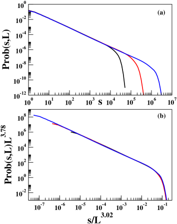
Figure 2: (Color online) The avalanche size distributions for three different system sizes $L=64$ (black), 128 (red) and 256 (blue) have been plotted on a double logarithmic scale in (a). The finite size scaling of the same data is shown in (b).

We argue that assigning a fixed boundary in the SOC models of earthquakes is rather artificial. In nature there is no fixed boundary for the earthquakes which absorbs earth’s vibrations, the seismic waves propagate in all directions till they slowly damp out at long distances. Presence of a fixed boundary introduces a strong non-uniformity in the system i.e., all measurable quantities show strong dependence on the distance from the boundary. This effect is present in both conservative as well as non-conservative versions of the OFC model, but it is so strong in the latter case that even arriving at the stationary state becomes very difficult Grassberger . It is therefore desirable that all avalanches are on the same footing with respect to the boundary and at the same time the origin of the avalanche should be at the farthest interior point of the system.

This argument prompted us to formulate a new boundary condition. Here, a globally fixed set of lattice sites does not constitute the boundary for all avalanches. In contrast, boundaries are different for different avalanches depending on the positions of the avalanche origins, and its position is constantly moved from one avalanche to the other.

First we make the square lattice periodic in both directions to get the topology of a torus. An arbitrary random distribution of forces $f_{i,j}$, drawn from a set of independent and identically distributed random numbers within $\{0,1\}$ are assigned at all $L^{2}$ sites. The maximum force $f_{max}$ among all $L^{2}$ sites is found to be at some specific location $(i_{o},j_{o})$ and the difference from the threshold force is estimated: $\delta=f_{c}-f_{max}$. Forces at all sites are then enhanced by $\delta$ so that at the origin $(i_{o},j_{o})$ the force reaches the threshold $f_{c}$. The avalanche then starts from the origin and a cascade of relaxations propagates away from the origin.

Now, for this avalanche, we select a specific set of lattice sites as the boundary such that the origin is at the center position with respect to these boundary sites. More precisely, on a $L\times L$ square lattice and with respect to the origin located at $(i_{o},j_{o})$ the boundary sites form two transverse rings on the torus defined by one column and one row of lattice sites as (Fig. 1):

$$i = i_{o}+L/2\hskip 11.38092pt{\rm mod}(L)\hskip 11.38092pt{\rm and}$$

$$j = j_{o}+L/2\hskip 11.38092pt{\rm mod}(L).$$ (6)

When a site adjacent to the boundary relaxes, it transfers $\alpha f_{i,j}$ force to every non-boundary neighbor but no force to the neigbor on the boundary. Therefore corrseponding to each boundary neighbor $\alpha f_{i,j}$ disappears from the system and in this way the system looses force.

Since the system is otherwise periodic in all directions all lattice sites are equivalent. Consequently all avalanches are also equivalent since all of them grow in similar surroundings. In a way this is similar to elimination of surface effects in a finite size system. Surface profiles for the averaged force per site $\langle f\rangle$, number of avalanche origins at each site $\langle e\rangle$ and average size of the avalanche per site $\langle s\rangle$ show uniform flat surfaces but within a very small fluctuation for all sites within the lattice $L\times L$. We are also studying other numerically challenging problems of SOC using moving boundary condition.

Figure 3: (Color online) Scaling of the waiting time distribution by the (a) Corral method (b) BCDS method. Symbols used for: $L=$ 64 (circle), 128 (square), 256 (triangle) and for $s_{c}=0$ (black), $8$ (red), $64$ (blue) and $512$ (magenta). Values of the scaling exponents used in (b) are $d_{f}$=1.67 and $b$=0.29. The continuous line is the best fit by the functional form in Eqn. (8).

Since in a single relaxation, the force at the site is reduced to zero, it creates the possibility that more than one site (typically two) can reach the threshold simultaneously. However, such situations occur with very low probability and in these cases we choose randomly one of the sites as the origin and construct boundaries with respect to this site but relaxation starts from both the unstable sites. Since the forces are continuously varying real numbers, the precision of the numbers is important as observed in Drossel . To ensure that the system has indeed reached the stationary state we calculated the average avalanche size $\langle s(L)\rangle$ for every 10000 avalanches and monitored its variation with time. This quantity first grows with time but eventually saturates. Repeating this calculation for different system sizes it is observed that the relaxation time grows as $L^{2}$.

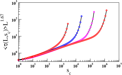
Figure 4: (Color online) The average recurrence time $\langle\tau(L,s_{c})\rangle$ has been plotted for different values of $s_{c}$ and multiplied by the system size dependent factor $L^{d_{f}}$. On increasing system size the plot approaches to the variation mentioned in Eqn. (10) with $b=0.30$.

First we present the results for the conservative case of $\alpha=1/4$. The avalanche size $s$ is the total number of relaxations in an avalanche and represents the total energy release in our model earthquake. ${\rm Prob}(s,L)$ is the probability that a randomly selected avalanche has size $s$. While for the infinitely large system size the distribution should indeed be a simple power law, for the finite size systems, a finite size scaling of the distribution is required:

$${\rm Prob}(s,L)\sim L^{-\mu}{\cal H}(s/L^{\nu})$$ (7)

where the scaling function ${\cal H}(x)\sim x^{-1-b}$ for $x\to 0$ and for $x>>1$, ${\cal H}(x)$ decreases faster than a power law so that, $b=\mu/\nu-1$. The system size dependence of the average avalanche size and durations are observed to be $\langle s(L)\rangle\sim L^{2.26}$ and $\langle T(L)\rangle\sim L^{0.63}$. This shows that the avalanche dynamics is sub-diffusive. We believe that this is due to fact that force is always reset to zero in a relaxation which initiates more relaxations and thus increases the size of the avalanche.

In Fig. 2(a) we show the plot of avalanche size distribution for three different system sizes $L$ = 64, 128 and 256 on the double logarithmic scale. All of them have very large portions of straight regions starting from very small sizes to the cut-off sizes. A scaling of the data with an excellent data collapse is shown in Fig. 2(b) yielding the values of $\nu=3.02$ and $\mu=3.78$ giving $b\approx 0.26$. Such a good power law behaviour as well as the excellent finite size scaling have been achieved only due to the moving boundary condition where all lattice sites as well as the avalanches are equivalent and have not been observed in fixed boundary cellular automata models of earthquakes before OFC ; Grassberger .

Since we have assumed that forces at all sites increase uniformly at unit rate, the time difference between successive avalanches is exactly equal to $\delta$. With this definition, the recurrence time distribution (RTD) ${\rm Prob}(\tau,s_{c},L)$ has been calculated for different system sizes $L$ as well as different $s_{c}$ values. The effects of $s_{c}$ and $L$ on RTD are competitive. For $s_{c}=0$, the RTD is simply the distribution of force increments $\delta$ only. Since the probability of occurrence of an avalanche of size at least $s_{c}$ decreases with $s_{c}$, for a fixed $L$ the recurrence time increases with increasing $s_{c}$. On the other hand for a fixed $s_{c}$, since the maximum of the avalanche sizes increases with $L$, the probability of occurrence of an avalanche of size at least $s_{c}$ increases with increasing $L$. Consequently the recurrence time decreases with increasing L.

In Fig. 3(a) we show an unified scaling of twelve different plots with the minimal value of the avalanche sizes measured $s_{c}=0,8,64$ and $512$ for three different system sizes $L$ =64, 128 and 256. Logarithmic binning is used for coarse-graining of the data. The average waiting time $\langle\tau(L,s_{c})\rangle$ is calculated for each plot. Following Eqn. (4) we then scale every plot with corresponding $\langle\tau(L,s_{c})\rangle=1/R$ and observe an excellent collapse of all twelve plots. This confirms the Corral scaling in our model. We tried to verify the Corral scaling form:

$${\cal G}(x)\sim x^{-a_{1}}\exp(-a_{2}x^{a_{3}})$$ (8)

and obtained $a_{1}=0.003$, $a_{2}=1.02$ and $a_{3}=0.99$ compared to $a_{1}=0.33$, $a_{2}=0.63$ and $a_{3}=0.98$ observed in Corral . The exponential tail in ${\cal G}(x)$ is consistent with the Gamma distribution observed by Corral but the observed power law decay component for small values of waiting times is rather absent in our model.

To see if BCDS scaling is also valid for our model, we plotted ${\rm Prob}(\tau,L,s_{c})(s_{c}^{b}/L^{d_{f}})$ vs. $\tau L^{d_{f}}/s_{c}^{b}$ and obtained a scaling form like:

$${\rm Prob}(\tau,L,s_{c})\frac{s_{c}^{b}}{L^{d_{f}}}\sim{\cal F}_{1}(\tau\frac{L^{d_{f}}}{s_{c}^{b}}).$$ (9)

Here also we see a very good collapse of the nine sets of data for three system sizes $L=64$, 128 and 256 and for $s_{c}=8,64$ and 512. The scaling exponents that gave the best collapse were tuned to $d_{f}=1.67$ and $b=0.29$. The best fit with the functional form in Eqn. (8) gives $a_{1}=0.001$, $a_{2}=3.21$ and $a_{3}=0.99$ again showing an exponential tail similar to that obtained from real data analysis Corral but without any power law component.

We therefore conclude that both the scaling forms used by Corral as well as BCDS are valid for scaling of the RTD data in our model. The scaling functions in both cases were observed to be very close to simple exponential decay and the power law part representing the RTD for small values of the recurrence times turned out to be absent. This result may also be compared with two recent analytical calculations: (i) a pure exponential decay of the RTD Molchan (ii) an approximate unified law compatible with the empirical observations incorporating the Omori law Saichev .

For Corral’s analysis it is the single parameter scaling i.e., the mean recurrence time $\langle\tau(L,s_{c})\rangle$. However this parameter in turn also depends jointly on the another two competitive parameters of the distribution, namely the system size $L$ and the avalanche size cut-off $s_{c}$ in the following way:

$$\langle\tau(L,s_{c})\rangle\propto\frac{s_{c}^{b}}{L^{d_{f}}}.$$ (10)

To check if it is really true we plotted $\langle\tau(L,s_{c})\rangle L^{d_{f}}$ with respect to $s_{c}^{b}$ for $L=32,64,128$ and 256 using $d_{f}=1.67$ in Fig. 4. A nice collapse of the data for the four different system sizes are observed for small and intermediate values of $s_{c}$. Collapse of the data between two successive system sizes increased with the system size. The slope of the curve in the longest straight region corresponds to $b=0.30$.

Finally, we studied the OFC model using values of $\alpha<1/4$ again on a square lattice of size $L$ using open but moving boundary condition. To our surprise we see that the dynamics become periodic after a short relaxation time of the order of $L^{2}$. This is checked by looking at the ‘hamming distance’. Starting from a random distribution of forces as before we skip some $10L^{2}$ initial avalanches and store the force configuration in an array $f_{store}$. After that at the end of every avalanche we calculated the maximal site difference ${\rm max}|f_{i,j}-f_{store}(i,j)|$ and measure the time when this maximal difference becomes less than a small number $\epsilon=10^{-12}$. The periodic time is of the order of $L^{2}$ but less than it, and found to depend on the initial distribution of force values.

To summarize, we have studied in a model the scale invariance properties observed in the real data of earthquakes over last several years by different groups. More specifically we studied a self-organized critical model of earthquakes using a square lattice cellular automaton. Using a moving boundary condition we could eliminate all boundary effects. We first observe that the avalanche size distribution of this model follow excellent finite size scaling. Further, the recurrence time distribution was analyzed in two ways, i.e., using Corral as well as BCDS scalings. We observe that our simulated data of the RTD support both scalings very well which leads us to conclude that the mean recurrence time is actually a joint function of both the system size as well as the avalanche size cut-off as used to measure the waiting times.

Electronic Address: manna@boson.bose.res.in

References

- (1) B. B. Gutenberg and C. F. Richter, Bull. Seismol. Soc. Am. 34, 185 (1944).
- (2) F. Omori, J. Coll. Sci. Imp. Univ. Tokyo, 7, 111 (1895).
- (3) P. Bak, K. Christensen, L. Danon, T. Scanlon, Phys. Rev. Lett. 88, 178501 (2002).
- (4) K. Christensen, L. Danon, T. Scanlon and, P. Bak, Proc. Natl. Acad. Sci. 99, 2509 (2002).
- (5) Á. Corral, Phys. Rev. Lett, 92, 108501 (2004).
- (6) Á. Corral, Phys. Rev. E, 68, 035102(R) (2003).
- (7) Y. Y. Kagan, Physica D, 77, 162 (1994).
- (8) P. G. Okubo and K. J. Aki, J. Geophys. Res. 92, 345 (1987).
- (9) J. Davidsen and M. Paczuski, Phys. Rev. Lett. 94, 048501 (2005).
- (10) M. Baiesi and M. Paczuski, Phys. Rev. E. 69, 066106 (2004).
- (11) R. Burridge and L. Knopoff, Bull. Seismol. Soc. Am. 57, 341 (1967).
- (12) P. Bak, C. Tang and K. Wiesenfeld, Phys. Rev. Lett, 59, 381 (1987).
- (13) P. Bak and C. Tang, J. Geophys. Res. 94, 15635 (1989).
- (14) Z. Olami, H. J. S. Feder and K. Christensen, Phys. Rev. Lett. 68, 1244 (1992).
- (15) P. Grassberger, Phys. Rev. E, 49, 2436 (1994).
- (16) J. X. de Carvalho and C. P. C. Prado, Phys. Rev. Lett. 84, 4006 (2000).
- (17) S. Lise and M. Paczuski, Phys. Rev. E 63, 036111 (2001).
- (18) B. Drossel, Phys. Rev. Lett. 89, 238701 (2002).
- (19) G. Molchan, Pure appl. geophys. 162, 1135 (2005).
- (20) A. Saichev and D. Sornette, arxiv:physics/0606001.