Detection of current-induced spins by ferromagnetic contacts

Abstract

Detection of current-induced spin accumulation via ferromagnetic contacts is discussed. Onsager’s relations forbid that in a two-probe configuration spins excited by currents in time-reversal symmetric systems can be detected by switching the magnetization of a ferromangetic detector contact. Nevertheless, current-induced spins can be transferred as a torque to a contact magnetization and affect the charge currents in many-terminal configurations. We demonstrate the general concepts by solving the microscopic transport equations for the diffuse Rashba system with magnetic contacts.

The notion that netto spin distributions can be generated by electric currents in the bulk of non-magnetic semiconductors with intrinsic spin-orbit (SO) interaction has been predicted Levitov ; Edelstein and experimentally confirmed Katoaccum . The related spin Hall effect, causing accumulations of spins at the edges, has also been observed exp . It can be extrinsic, i.e. caused by impurities with SO scattering DP ; extrinsic or intrinsic due to an SO split band structure Murakami ; Sinova . However, all experiments to date detected the current-induced spins optically metal . An important remaining challenge for theory and experiment is to find ways to transform the novel spin accumulation (SA) and spin currents (SCs) into voltage differences and charge currents in micro- or nanoelectronic circuits in order to fulfill the promises of spintronics.

In this Letter, we address the possibility to generate a spin-related signal to be picked up by ferromagnetic contacts. This signal can be in the form of a voltage change or a torque acting on the magnetization of the ferromagnet (FM). In practice, this raises technical difficulties due the conductance mismatch Schmidt that can be solved Crowell and are not addressed here. We rather focus on conceptual problems that are related to the voltage and torque signals generated by current-induced spins vanWees . The Onsager relations for the conductance Onsager forbid voltage based detection of current-induced spins by a ferromagnetic lead in a two-probe setup within linear response. We sketch a microscopic picture of the physics and formulate a semiclassical scheme in the diffuse limit. We address spin detection in a multi probe geometry, calculate the Hall conductivity and compare it to the anomalous Hall effect. We also discuss the possibility to construct spin filters not based on FMs, but on conductors with spatially modulated SO interactions.

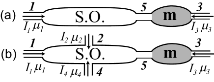
Figure 1: Current-Voltage configuration for (a) two- and (b) four-probe setup.

We first address the symmetry properties in terms of the Onsager relations for the (linear) conductance Onsager ; REF:Casimir ; REF:Buttiker86 ; REF:Hankiewicz . A generic SO-Hamiltonian $H$ involves products of velocity and spin operators that are invariant under time reversal. Even when spin-degenerate bands are split due to a broken inversion symmetry, the Kramers degeneracy remains intact. The Hamiltonian of the combined SO$|$F system has the symmetry $TH(\mathbf{m})T^{-1}=H(-\mathbf{m})$, where $\mathbf{m}$ is a unit vector in the direction of the magnetization of the FM and $T$ the time-reversal operator. We now focus on a general multi-probe setup (see Fig. 1b for a 4-probe setup). The currents in the leads and the respective chemical potentials of the reservoirs are related in linear response as $I_{i}=\sum_{j}G_{ij}\mu_{j}$. The elements of the conductance matrix can then be expressed as a commutator of the respective current operators $\hat{I}_{i}(t)$ and $\hat{I}_{j}(t)$ in the leads $i$ and $j$: $G_{ij}=\lim_{\omega\rightarrow 0}\mathrm{Re}\,\int_{0}^{\infty}dt(e^{i\omega t}/\omega)\langle[\hat{I}_{i}(t),\hat{I}_{j}(0)]\rangle,$ where the brackets $\langle\cdots\rangle$ denote either ground state expectation value or thermal averaging. For reversed magnetization we can relate the states that enter the averaging with those of the original magnetization using $T$. By inserting $T^{-1}T$ between the operators in the Kubo formula it follows $G_{ij}(-\mathbf{m})=G_{ji}(\mathbf{m})$. For the two-probe configuration (Fig. 1a), the currents in the two leads are equal and opposite, by current conservation, and there is only one conductance $G$. This implies $G(\mathbf{m})=G(-\mathbf{m})$. Thus, it is not possible to detect the SA by reversing the magnetization or current direction in this case.

Voltage signals can be measured in a three or more terminal setup, however. We focus on the current/voltage configuration in Fig. 1b with $I_{1}=-I_{3}$, $I_{2}=-I_{4}$, $eV_{1}=\mu_{3}-\mu_{1}$ and $eV_{2}=\mu_{4}-\mu_{2}$ REF:Casimir appropriate, e.g., to a set up where leads 2 and 4 are connected together by a resistor, while leads 1 and 3 are connected by a battery. Then $I_{i}=\sum_{j=1,2}(-1)^{i+j}\alpha_{ij}V_{j}$, where the coefficients $\alpha_{ij}$ can be found in Eqs. (4.a-4d) of Ref. REF:Buttiker86 . The Onsager relations can then be expressed as: $\alpha_{ij}(\mathbf{m})=\alpha_{ji}(-\mathbf{m})$. If we choose (say) $I_{1}=0$, the relation between the applied current and the spin-Hall voltage is: $I_{2}=V_{1}(\alpha_{11}\alpha_{22}-\alpha_{12}\alpha_{21})/{\alpha_{12}}$. Upon switching the magnetization direction we obtain the same formula except for the change of $\alpha_{21}$ to $\alpha_{12}$ and vice versa: $G_{H}(\mathbf{m})=\frac{\alpha_{21}}{\alpha_{12}}G_{H}(-\mathbf{m}).$ Since in general $\alpha_{21}\neq\alpha_{12},$ $G_{H}$ changes as $\mathbf{m}$ is switched. Our analysis implies the equivalence of two Hall measurements: (i) setting $I_{1}$ to zero and detecting $V_{1}$ generated by an applied $I_{2}$ and (ii) setting $I_{2}$ equal to zero and detecting $V_{2}$ Valenzuela . In other words, driving a current $I_{2}$ through the system and detecting the spin Hall voltage with a ferromagnetic contact is equivalent to driving a SA into the SO region via a FM that leads to a real Hall voltage detectable by normal contacts. We note that the symmetries of the joint SO$|$F region is identical to a bulk FM with SO interaction. A SC cannot be detected by merely switching $\mathbf{m}$ or current direction in a two-probe setup Ref:AHE .

Further insight to the Onsager relations can be obtained by considering the microscopic scattering processes at the SO$|$F interface. For simplicity, we take the FM to be halfmetallic and with a matched electronic structure, i.e., electrons with spin parallel (antiparallel) to $\mathbf{m}$ are transmitted (reflected). The conductance is proportional to the sum of transmission probabilities including multiple scattering processes at the SO$|$F interface and impurities. When the spin polarized by the point contact is a majority electron in the FM, it is directly transmitted with probability unity. When we reverse the magnetization direction, the electron is initially completely reflected. However, the reflected electron subsequently scatters at impurities, experiencing the effective Zeeman field due to the SO coupling that causes the spin to precess. It eventually approaches the interface again with a different spin orientation. Only the component parallel to the majority spin direction is transmitted. For the reflected antiparallel component the game starts all over again. By repeated scattering at the interface, the electron is eventually transmitted for both magnetization directions with equal probability. Note the similarity of this picture with the reflectionless tunneling at a superconducting interface REF:reflesstunn . An electron reflected once at a ferromagnetic Hall contact, on the other hand, has a finite probability to escape into the drain, thus leaving a voltage signal of its spin. When the SC is generated by a point contact and injected into a ballistic normal conductor Eto the argument is clearer: although an up-spin electron leaving the point contact is reflected by an attached FM with antiparallel magnetization, the subsequent spin-flip reflection at the point contact leads to a transmission probability that is the same for a parallel magnetization, in agreement with the Onsager relations.

We now focus on a microscopic transport theory for a simple model Hamiltonian, the Rashba spin-split two-dimensional electron gas (R2DEG) with SO coupling $H^{R}=(\alpha/\hbar)\mathbf{p}\cdot({\bm{\sigma}}\times\hat{\bm{z}})$, where $\mathbf{p}$ is the momentum operator, $\{\sigma_{i}\}$ are the Pauli spin matrices, and $\alpha$ parameterizes the strength of the SO interaction. For a setup as in Fig. 1 and in the diffuse limit with spin-independent s-wave scatterers we compute the voltage signal in the ferromagnetic lead. The diffusion equation for the (momentum-integrated) density matrix $\rho(E)=n(E)+\mathbf{s}(E)\bm{\cdot\sigma}$ has been obtained by Ref.s Mishchenko ; Burkov . We use the notation of Ref. inanc for diffusion equations (Eq.s (6-8) in Ref. inanc ) and for the expression of SC in terms of $\rho(E)$ (Eq.(9) in Ref. inanc ). We define $L_{s}=\sqrt{D\tau_{s}}$, $\lambda=K_{s-c}/D$ and $\eta=K_{p}L_{s}/D$. These diffusion equations are the leading terms in a gradient expansion, and require for their validity that the SA gradient is small compared to the transport mean free path $v_{F}\tau$. Generally, this requires $L_{s}>v_{F}\tau$ and results strictly hold only in the dirty limit, $\xi\ll 1$. Nevertheless, since results are well behaved for all $\xi$ they might be useful beyond the regime of formal validity. We consider a weak FM with diffusion equation $\nabla^{2}s_{m}=s_{m}/L_{sF}^{2}$ for the SA component $s_{m}$ parallel to the magnetization, where $L_{sF}$ is the spin-flip relaxation length in the FM. The charge and SCs in the FM read $\mathbf{j}(E)=-\nu_{F}D_{F}(\bm{\nabla}n+\delta D\bm{\nabla}s_{m})$ and $\mathbf{j}^{m}(E)=-\nu_{F}D_{F}\big{(}\bm{\nabla}s_{m}+(\delta D/4)\bm{\nabla}n\big{)}$ where $\nu_{F}D_{F}=(\nu_{+}D_{+}+\nu_{-}D_{-})/2$, $\delta D=(\nu_{+}D_{+}-\nu_{-}D_{-})/(\nu_{F}D_{F})$, $\nu_{\pm}$ and $D_{\pm}$ are the density of states and diffusion constants of the majority and minority spin electrons.

We chose a simple model for the matching conditions between a R2DEG and a FM: the charge current as well as the SC polarized in the magnetization direction of the FM are conserved at the interface, whereas the SC polarized perpendicularly to the magnetization direction transfers a torque onto the magnetization by being absorbed at the interface Slonczewski ; Nunez . We have a now complete set of matching/boundary conditions at the R2DEG$\mid$F interface: $m_{i}(\bm{n}\cdot\bm{j}_{R}^{i})=m_{i}(\bm{n}\cdot\bm{j}_{F}^{i}),$ $\bm{m}\times\bm{s}_{R}=0$ and $\bm{m}\cdot\bm{s}_{R}=\bm{m}\cdot\bm{s}_{F}$, where the subscripts F and R refer to the FM and the R2DEG respectively. The first condition holds when the interface does not cause additional spin relaxation. The second one requires that the perpendicular SC is dephased in the FM on a length scale that is much smaller than the mean free path. The third condition, i.e. continuity of the SA in the magnetization direction, has been useful for purposes of illustration before old ; Kovalev , but does not hold for general interfaces Galitski .

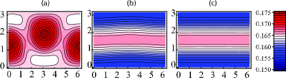
Figure 2: The potential drop in units of $J_{p}\delta D^{2}L_{s}/4D\nu_{R}$ as a function of the magnetization direction for $\Gamma(1-\delta D^{2}/4)=5$ and $\xi=0.2$ (a), $\xi=1$ (b) and $\xi=5$ (c). The $y$-axis is the azimuthal angle $\theta$ and $x$-axis is the polar angle $\phi$ of $\mathbf{m}$.

Solving the diffusion equations with boundary conditions is simplified by decomposing the SC across the interface into an injection current from the FM and an out-diffusion current of the SA in the R2DEG. The former is a linear function of $\mathbf{m}$ while the latter depends on the bulk SA direction. We define two vector functions $\bm{\mu}$ and $\mathbf{f}$ at point $\mathbf{r}$ at the interface as the $\mathbf{m}$-dependent and independent part of the normal derivative of $\mathbf{s}$:

$$L_{s}(\mathbf{n}\cdot\bm{\nabla})s_{i}|_{r}=\big{(}\mu_{i}(\mathbf{m})|\mathbf{s}|+\lambda L_{s}^{2}(\mathbf{z}\times\mathbf{J}_{p})_{i}f_{i}/D\nu_{R}\big{)}\big{|}_{r}$$

Here $\mu_{i}$ is a linear function of $\mathbf{m}$, $\mathbf{n}$ is the unit normal vector at the interface, and $\mathbf{J}_{p}$ is the local current density.

For a (wide contact) two-terminal configuration $\mathbf{n}$, $\mathbf{J}_{p}$, $\bm{\mu}$ and $\mathbf{f}$ are constant over the interface. We choose the $x$-direction to be the current direction and $y$-direction parallel to the interface. We then obtain the SA at the interface to order $(\alpha/k_{F})^{2}$ as:

$$\mathbf{s}|_{0} =\mathbf{m}J_{p}(\delta D/4-m_{y}\lambda L_{s})/\Lambda\left(\mathbf{m}\right),$$ (1)

$$\Lambda\left(\mathbf{m}\right) =L_{s}^{-1}D\nu_{R}\mathbf{m}\cdot\bm{\mu}+L_{sF}^{-1}D_{F}\nu_{F}(1-\delta D^{2}/4).$$ (2)

Here, $\mu_{x}=(\sqrt{2}-1)(\kappa_{+}+\kappa_{-})m_{x}-(2-\sqrt{2})2\eta m_{z}$, $\mu_{y}=m_{y}$ and $\mu_{z}=2\eta(\sqrt{2}-1)m_{x}+(2-\sqrt{2})(\kappa_{+}+\kappa_{-})m_{z}$, where $2\kappa_{\pm}^{2}=3-4\eta^{2}\pm(1-24\eta^{2}+16\eta^{4})^{1/2}$ and $\mathrm{Re}\kappa_{\pm}>0$. Note that these expressions do not depend on $f_{i}$. In contrast to the SA at the interface the potential drop $\phi_{FR}=-J_{p}\delta D^{2}/8\Lambda$ is invariant under $\mathbf{m}\rightarrow-\mathbf{m}$, consistent with the Onsager relations (Fig. 2). In the clean limit, the terms that do not involve $m_{z}$ agree with previous results in the absence of SO interaction old . The anomalous $m_{z}$ dependence is due to a different spin relaxation length for the $z$-component of the spin. A similar effect has been observed in numerical simulations Pareek . Although $\phi_{FR}$ does not depend on the direction of $\mathbf{m}$ in the $xy$-plane, all higher order corrections in $\alpha/k_{F}$ have an even angular dependence. The resistance modulation differs from the tunneling magnetoresistance found by Rüster et al. Ruester in that here the SO interaction is in the normal metal rather than in the FM.

As shown above, the spin Hall voltage does not need to be invariant under reversal of the magnetization of the FM. Using the same diffusion equations, we calculate the extra potential drop $\phi_{H}$ at a ferromagnetic “Hall” lead. Now the interface of the contact lies parallel to the (bulk) current direction $x$. When the charge current through the ferromagnetic lead is biased to zero, we obtain

$$\phi_{H}=\frac{J_{p}^{\prime}\delta D}{2\Lambda}\left(\frac{\alpha\xi\mathbf{m}\cdot\mathbf{f}}{v_{F}\sqrt{1+4\xi^{2}}}-\frac{m_{z}\xi^{2}}{4\pi\hbar D\nu_{R}(1+4\xi^{2})}\right),$$

that changes sign with the magnetization direction. Here $J_{p}^{\prime}$ is the local average current density parallel to the Hall lead, $\mu_{x}=m_{x}$, $\mu_{y}=(\sqrt{2}-1)(\kappa_{+}+\kappa_{-})m_{y}-(2-\sqrt{2})2\eta m_{z}$, $\mu_{z}=2\eta(\sqrt{2}-1)m_{y}+(2-\sqrt{2})(\kappa_{+}+\kappa_{-})m_{z}$, $f_{x}=0$, $f_{y}=(\kappa_{+}+\kappa_{-})(\sqrt{2}-1)$, and $f_{z}=(\sqrt{2}-1)2\eta$.

We now focus on the transverse component of the angular momentum that is transferred to the FM as a torque on the magnetization Slonczewski ; Nunez , which is not restricted to certain symmetries under reversal of $\mathbf{m}$ by the Onsager relations. For the two-probe setup, we obtain:

$$\tau_{i} =J_{p}\lambda L_{s}\Bigg{[}\delta_{i2}-m_{y}m_{i}+\frac{D_{R}\nu_{R}}{L_{s}\Lambda}\left(\frac{\delta D}{4\lambda L_{s}}-m_{y}\right)$$

$$\times\left(\mu_{i}-m_{i}(\mathbf{m}\cdot\bm{\mu})-\eta^{1/3}(\delta_{i3}m_{x}-\delta_{i1}m_{z})\right)\Bigg{]}$$ (3)

We notice both even and odd contributions under magnetization reversal. Their ratio is controlled by the dimensionless parameter $\zeta=\delta D/4\lambda L_{s}$ and the parameter related to the conductance mismatch $\Gamma=\nu_{F}D_{F}L_{s}/\nu_{R}D_{R}L_{sF}$, both typically much larger than unity. For $\zeta\ll\Gamma$ $\left(\zeta\gg\Gamma\right)$ the torque is an even (odd) function of $m_{i}$. For general parameters the torque displays a surprising complexity (Fig. 3). In the limit $\zeta\ll\Gamma$, the even terms dominate and it is possible to switch the magnetization by a charge current. The switching dynamics will be complicated by the odd terms if $\zeta\lesssim\Gamma$. These effects are rotating $\mathbf{m}$ around the accumulation direction (which is due to spin precession in the SO region and is due to the term proportional to $\eta^{1/3}$ in the expression above), and pulling $\mathbf{m}$ out of the plane depending on whether $m_{z}$ is greater than or less than zero.

Assuming a nm scale thick ferromagnetic film (such as Fe) on InAs in the clean limit, we estimate, using Slonczewski’s expressions Slonczewski , the critical current density for magnetization-switching to be of the order of $10^{0}\mathrm{A/cm}$ (equivalent to a bulk current density of $10^{6}\mathrm{A/cm^{2}}$). This result will increase by a factor $g_{S}/g$, where $g_{S}$ and $g$ are the Sharvin and total spin conductance of the contact respectively. It is possible to reduce critical currents strongly by reducing the magnetization of FM. This can be achieved by choosing a ferromagnetic semiconductor (that should be n-type in the case or InAs Kio ) that is furthermore close to its Curie temperature Chiba . Excessive heating can be avoided by short-time pulses Chiba . Small-angle magnetization dynamics is induced at much smaller currents and can be detected optically for e.g. a three-terminal geometry. Finally, we mention that dominant SO coupling in 2D heavy hole gas has a $k^{3}$ dependence which does not generate any bulk SA SAhole . Therefore SA effects predicted here will be relatively weak for most 2DHGs. The $k$-linear SO coupling can be increased in 2DHGs by applying strain.

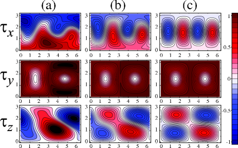
Figure 3: Components of the spin transfer torque, scaled by a factor $J_{p}\lambda L_{s}$, plotted for the set of parameters $\xi=1$, $\zeta=5$ and (a) $\Gamma=1$, (b)$\Gamma=5$ and (c) $\Gamma=25$. The $y$-axis is the azimuthal angle $\theta$ and $x$-axis is the polar angle $\phi$ of $\mathbf{m}$.

We finally note that spin filters can be fabricated without FMs by spatial modulation of the SO coupling. This can be useful for the R2DEG in which $\alpha$ can be modulated by an electric field. In a symmetric but externally gated quantum well, the inversion-symmetry-breaking electric field, and thus the sign of $\alpha$ can be reversed. The region in which $\alpha$ is reversible would be able to detect the SC generated in another one, since the resistance of the $\alpha|\alpha$ junction differs from that of the $\alpha|-\alpha$ junction.

In conclusion, we addressed current-induced spin related voltage and torque signals in ferromagnetic contacts. We presented the conductance and spin transfer torque due to the spin-polarized currents generated in a spin-orbit coupled region in two- and many-terminal devices and discussed their symmetry properties in terms of the Onsager relations. Symmetry prohibits the detection of spins in two-probe conductance measurement via a magnetization switch. In contrast, it is possible to detect a torque signal, distinctive of SCs, even in a two probe setting. For the four-probe Hall type measurement, both current induced SA and the spin Hall current may be detected by voltages, where the contribution of the spin Hall current to the Hall conductivity bears close similarity to the anomalous Hall effect.

B.I.H. would like to thank H.-A. Engel and E. G. Mishchenko for useful discussions. This work was supported by the FOM, EU Commission FP6 NMP-3 project 05587-1 “SFINX”, NSF grants PHY-0117795 and DMR-0541988 and NSERC discovery grant number R8000.

References

- (1) F. T. Vas’ko and N. A. Prima, Sov. Phys. Solid State 21, 994 (1979); L.S. Levitov et al., Zh. Eksp. Teor. Fiz. 88, 229 (1985).
- (2) V. M. Edelstein, Sol. Stat. Commun. 73, 233 (1990); J.I. Inoue et al., Phys. Rev. B 67, 033104 (2003).
- (3) Y.K. Kato et al., Nature 427, 50 (2004); Y.K. Kato et al., Phys. Rev. Lett. 93, 176601 (2004); In hole systems: A. Yu. Silov et al., Appl. Phys. Lett. 85, 5929 (2004); S. D. Ganichev et al., cond-mat/0403641 (unpublished).
- (4) Y.K. Kato et al., Science 306, 1910 (2004); J. Wunderlich et al., Phys. Rev. Lett. 94, 047204 (2005); V. Sih et al., Nature Phys. 1, 31-35 (2005).
- (5) Several very recent experiments report electric signals of the extrinsic spin Hall effect in metals : E. Saitoh et al., Appl. Phys. Lett. 88, 182509 (2006); S.O. Valenzuela and M. Tinkham, Nature 442, 176–179 (2006); T. Kimura et al., cond-mat/0609304.
- (6) M.I. Dyakonov and V.I. Perel, JETP Lett. 33, 467 (1971).
- (7) J. E. Hirsch, Phys. Rev. Lett. 83, 1834 (1999); S. Zhang, Phys. Rev. Lett. 85, 393 (2000); R.V. Shchelushkin and A. Brataas, Phys. Rev. B 71, 045123 (2005); J. Hu et al., Int. J. Mod. Phys. B 17, 5991 (2003) ; S.-Q. Shen, Phys. Rev. B 70, 081311(R) (2004); D. Culcer et al., Phys. Rev. Lett. 93, 046602 (2004); N.A. Sinitsyn et al., Phys. Rev. B 70, 081312 (2004); A.A. Burkov et al., Phys. Rev. B 70, 155308 (2004).
- (8) S. Murakami et al., Science 301, 1348 (2003); Phys. Rev. B 69, 235206 (2004).
- (9) J. Sinova et al., Phys. Rev. Lett. 92, 126603 (2004).
- (10) G. Schmidt et al., Phys. Rev. B 62, R4790 (2000).
- (11) X. Lou et al., cond-mat/0602096; P. Crowell c.s., unpublished; P. Cheng et al., cond-mat/0608453
- (12) B. J. van Wees, Phys. Rev. Lett. 84, 5023 (2000); P. R. Hammar et al., Phys. Rev. Lett. 84, 5024 (2000)
- (13) L. Onsager, Phys. Rev. B 38, 2265 (1931)
- (14) H. B. G. Casimir, Rev. Mod. Phys. 17, 343 (1945).
- (15) M. Büttiker, Phys. Rev. Lett. 57, 1761 (1986).
- (16) Onsager-like relations have been discussed, assuming an inversion symmetric setup, by E. M. Hankiewicz et al., Phys. Rev. B 72, 155305 (2005).
- (17) The spin-Hall signal in metallic devices metal has been measured by configuration (ii).
- (18) J. Inoue and H. Ohno, Science 309, 2004 (2005).
- (19) I. K. Marmorkos et al., Phys. Rev. B 48, 2811 (1993); C. W. J. Beenakker et al., Phys. Rev. Lett. 72, 2470 (1994); B. J. van Wees et al., Phys. Rev. Lett. 69, 510 (1992);
- (20) M. Eto et al., J. Phys. Soc. Jap. 74, 1934 (2005); P.G. Silvestrov and E.G. Mishchenko, Phys. Rev. B 74, 165301 (2006)
- (21) J.C. Slonczewski, J. Magn. Magn. Mater. 159, L1 (1996).
- (22) A. S. Núñez and A.H. MacDonald, Sol. State Commun. 139, 31 (2006).
- (23) E.G. Mishchenko et al., Phys. Rev. Lett. 93, 226602 (2004).
- (24) A.A. Burkov et al., Phys.Rev. B 70, 155308 (2004).
- (25) İ. Adagideli and G.E.W. Bauer, Phys. Rev. Lett. 95, 256602 (2005).
- (26) A. A. Kovalev et al., Phys. Rev. B 66, 224424 (2002).
- (27) V. M. Galitski et al., cond-mat/0601677.
- (28) M. Johnson and R. H. Silsbee, Phys. Rev. Lett. 55, 1790 (1985); P. C. van Son et al., Phys. Rev. Lett. 58, 2271 (1987).
- (29) T.P. Pareek, Phys. Rev. B 70, 033310 (2004)
- (30) C. Rüster et al., Phys. Rev. Lett. 94, 027203 (2005)
- (31) J.I. Inoue et al., Phys. Rev. B 70, 041303(R) (2004).
- (32) S. Murakami, Phys. Rev. B 69, 241202(R) (2004).
- (33) G. Kioseoglou et al., Nature Materials 3, 799 (2004).
- (34) D. Chiba et al., Phys. Rev. Lett., 93, 216602 (2004).
- (35) A. V. Shytov et al., Phys. Rev. B 73, 075316 (2006); T. L. Hughes et al., cond-mat/0601353 ; O. Bleibaum, S. Wachsmuth, cond-mat/0602517.