Non-resonant Raman response of inhomogeneous structures in the electron doped $t-t^{\prime}$ Hubbard model

Abstract

We calculate the non-resonant Raman response, the single particle spectra and the charge-spin configuration for the electron doped $t-t^{\prime}$ Hubbard model using unrestricted Hartree-Fock calculations. We discuss the similarities and differences in the response of homogeneous versus inhomogeneous structures. Metallic antiferromagnetism dominates in a large region of the $U-n$ phase diagram but at high values of the on-site interaction and for intermediate doping values inhomogeneous configurations are found with lower energy. This result is in contrast with the case of hole doped cuprates where inhomogeneities are found already at very low doping. The inhomogeneities found are in-phase stripes compatible with inelastic neutron scattering experiments. They give an incoherent background in the Raman response. The $B_{2g}$ signal can show a quasiparticle component even when no Fermi surface is found in the nodal direction.

I Introduction

Electron and hole doped cuprates share a similar phase diagram with antiferromagnetic and superconducting phases. However there are quantitative differences between them. While electron-doped show commensurate antiferromagnetismshirane in a large region of the $U-n$ phase diagram there is a quick suppression of antiferromagnetism in hole-doped cuprates. There it is well established that inhomogeneities appear when doping the Mott insulator. Among them the stripes, where holes are aligned in a row, have acquired importance as a possible scenario to explain the phase diagram of the hole doped cuprateskivelson . The strongest experimental support for stripes comes from neutron scattering experimentsNScatTr that show incommensurate peaks. They have been interpreted as coming from anti-phase stripes where the line of holes separate antiferromagnetic domains of opposite sign. The case of the electron doped cuprates is less clear. The signal obtained in neutron scattering experiments is commensurateNScat what would be compatible with in-phase inhomogeneities. This possibility can convene with theoretical predictions that incommensurate solutions will be more favored in hole than in electron dopingtohmaek94 ; leung94 ; moreo ; zhang ; oles . Very recent measurements of thermal conductivity and neutron scatteringando in electron doped cuprates have been interpreted as in-phase stripes while experiments of Nuclear Magnetic Resonancegorkov were seen as signatures of inhomogeneous structures. A low temperature pseudogap detected with tunneling spectroscopynaturetunn points to the presence of a ground state other than superconductivity whose origin could rely in inhomogeneous configurations.

In this work we perform a systematic analysis of homogeneous versus inhomogeneous structures in the electron doped $t-t^{\prime}$ Hubbard model using unrestricted Hartree-Fock (UHF) calculations. Stripes and inhomogeneities were predicted as a solution of the Hubbard model with $t^{\prime}=0$ using UHF approximationuhfstr . Within this framework we compute the spectral function and the non-resonant Raman response of the different configurations. In the study of commensurate antiferromagnetism it is interesting to have charge sensitive probes as the non-resonant Raman response which can detect charge order due to the possible selection of different regions of the Brillouin zonedicastro . Inhomogeneous solutions in electron doped have been studied previously with UHF in the three band Hubbard modelthreeband where they found that diagonal anti-phase stripes were the configuration lowest in energy. So far there are no evidence of these stripes in the experiments. We will use the simplest $t-t^{\prime}$ Hubbard model which has shown to be able to explain the pseudogap and the phase diagram of electron dopedtremblay cuprates and to give the correct low energy physics when compared with the two-band Hubbard modeltwobands . The $t-t^{\prime}$ Hubbard model has also been studied with UHF in the pastus ; normand where it was pointed out that $t^{\prime}$ favors homogeneous solutions in the electron doped case in contrast to the hole-doped. This was claimed to be due to the fact that $t^{\prime}$ does not frustrate the antiferromagnetism in the electron doped case as was also proven with other techniques as exact diagonalization in the electron doped $t-t^{\prime}-J$ modeltohyama ; leung and in Quantum Monte Carlo calculations of the $t-t^{\prime}$ Hubbard modelmoreo ; huang . Metallic antiferromagnetism has been found in experimentsonose . Our calculations agree with the former results that homogeneous antiferromagnetism is more stable in the electron than in hole doped case but in this systematic study we have found that for large enough values of the on-site interaction $U=6t-8t$ and at intermediate doping in-phase inhomogeneous configurations have the lowest energy. This is in strong contrast with what happens in the hole doped case where inhomogeneities are already found very close to half-fillingus . The result is compatible with the recent theoretical proposal of phase separation at intermediate fillingsarrigoni . Phase separation has also been claimed for the electron doped $t-t^{\prime}-J$ modelleung94 . Unrestricted Hartree-Fock can work better to explore the electron doped cuprates than the hole doped cuprates because when doping the $t-t^{\prime}$ Hubbard model with electrons we fill the wider upper antiferromagnetic band where quantum fluctuations are expected to be less important.

ARPES experiments in electron dopedarmitage cuprates show a Fermi surface made of electron pockets for dopings of $x=0.04$, $x=0.10$ and $x=0.15$ as expected from long range antiferromagnetic ordermoreo ; kusko . They also see the emergence of a hole-like Fermi surface around the nodal direction at $x=0.15$. This nodal signal seems to indicate the instability of the antiferromagnetismstability ; tremblay . As we work in the strong coupling limit we do not obtain the hole-like Fermi surface at $x=0.15$. It is known that to get it in mean-field calculations unrealistic values of $U$ are neededkusko . This case has been explored with different techniques where quantum fluctuations are properly taken into account (see tremblay ; hanke ; yuan ) but these techniques are not well suited for studying inhomogeneities. On the other hand ARPES also indicates the presence of spectral weight in the insulator gap. Theoretically, these midgap states have been obtained by adding spin fluctuations to the mean field solutionrice . Inhomogeneous configurations also form midgap states which would be an alternative explanation of these states.

A related issue concerns recent puzzling experimental results of electron-doped cuprates. Although the Fermi surface found in ARPES for most of the electron-doped cuprates lies in the antinodal direction, recent Raman experiments have found that coherent quasi-particles mainly reside in the nodal direction of the Brillouin zoneramansc in all the samples that they have analyzed ($x=0.135$, $x=0.147$ and overdoped samples). In particular they see that the $B_{2g}$ signal which involves averages mostly over the nodal region has a stronger quasiparticle component than the $B_{1g}$ signal which deals with the antinodal. Both signals show an incoherent background. In our calculations we find cases of inhomogeneous configurations that present a quasiparticle-like signal in the $B_{2g}$ Raman response although the Fermi level does not cross the nodal region. We argue that this is an example of a case in which two-particle properties cannot be induced from one-particle properties. We also find that inhomogeneities provide an incoherent background to the Raman response absent in the case of homogeneous metallic antiferromagnetism. Our results are qualitative. We do not pretend to do a close comparison with experiments for what we would have to take into account other very important effects as quantum fluctuations, scattering by impurities etc. We intend to find out the prints of inhomogeneities in the Raman signal.

The organization of this paper is as follows. In section II we review the $t-t^{\prime}$ Hubbard model and the unrestricted Hartree-Fock method. In Sect. III we discuss the $U-n$ phase diagram. Sect. IV gives the results obtained on one-particle properties and Section V deals with the electronic Raman response. In section VI we present our conclusions and open problems.

II The model and the method

The $t-t^{\prime}$ Hubbard model is defined in the two dimensional squared lattice by the hamiltonian

$$H=-t\sum_{<i,j>s}c^{+}_{is}c_{js}-t^{\prime}\sum_{<<i,j>>s}c^{+}_{is}c_{js}+U\sum_{i}n_{i\uparrow}n_{i\downarrow},$$ (1)

which gives rise to the dispersion relation

$$\varepsilon({\bf k})=-2t\;[\cos(k_{x}a)+\cos(k_{y}a)]-4t^{\prime}\cos(k_{x}a)\cos(k_{y}a).$$

$t>0$ and $t^{\prime}=-0.3t$ are generic values for modeling the physics of the cuprates. We will consider electron doping ($n>1$). We work in lattices of different sizes with periodic boundary conditions depending on the problem at hand. We obtain the $U-n$ phase-diagram working in a $L=14\times 14$ lattice. We use a $16\times 16$ lattice to discuss in-phase versus off-phase configurations and a $L=24\times 24$ lattice to compute the spectral function and the Raman response. A comparison of the results on the different lattice sizes for homogeneous and inhomogeneous configurations is done in the next section. The unrestricted Hartree-Fock approximation minimizes the expectation value of the hamiltonian (1) in the space of Slater determinants. These are ground states of a single particle many-body system in a potential defined by the electron occupancy of each site. This potential is determined self-consistently

$$H = -\sum_{i,j,s}t_{ij}c^{\dagger}_{is}c_{js}-\sum_{i,s,s^{\prime}}\frac{U}{2}{\vec{m}}_{i}c^{\dagger}_{is}{\vec{\sigma}}_{ss^{\prime}}c_{is^{\prime}}$$ (2)

$$+\sum_{i}\frac{U}{2}q_{i}(n_{i\uparrow}+n_{i\downarrow})+{\displaystyle c.c.},$$

where $t_{i,j}$ denotes next, $t$, and next-nearest, $t^{\prime}$, neighbors, and the self-consistency conditions are

$${\vec{m}_{i}}=\sum_{s,s^{\prime}}<c^{\dagger}_{is}{\vec{\sigma}}_{ss^{\prime}}c_{is^{\prime}}>,\;\;\;q_{i}=<n_{i\uparrow}+n_{i\downarrow}-1>,$$

where ${\vec{\sigma}}$ are the Pauli matrices.

We will call $E_{\lambda}$ where $\lambda=1\ldots 2L$ the eigenvalues of the hamiltonian and $u_{1}^{\dagger}|0\rangle,\ldots,u_{2L}^{\dagger}|0\rangle$ the basis that diagonalizes the hamiltonian. These fermionic operators are obtained from the original ones through:

$$c_{js}=\sum_{\lambda}U_{js,\lambda}u_{\lambda}.$$ (3)

III $U-n$ phase diagram

We have built a detailed $U-n$ phase diagram for $t^{\prime}=-0.3t$, which it is shown in Fig. 1 by comparing the energies of paramagnetic, antiferromagnetic and inhomogeneous configurations in a $14\times 14$ lattice size. Antiferromagnetism prevails over most of the phase diagram and inhomogeneities (VS in Fig. 1 ) can be found at intermediate doping and for high values of $U$. For the inhomogeneous solutions we have compared diagonal (DS) and vertical (VS) in-phase stripes, in-phase antiferromagnetic domains (DOM) and polarons (POL). Fig. 2 shows the comparison of the energies per particle for $U=8t$ and $t^{\prime}=-0.3t$. All these inhomogeneous solutions converge for $n=1.15$ where no antiferromagnetism can be found. In fact, antiferromagnetism does not converge in all the VS region in the phase diagram of Fig. 1. This is a clear indication that there is a critical density where inhomogeneities are preferred over homogeneous antiferromagnetism in unrestricted Hartree-Fock. The inhomogeneous solution lowest in energy consists of in-phase vertical stripes (VS) represented in Fig. 3 (up) in a $24\times 24$ lattice. In-phase antiferromagnetic domains (DOM) are very close in energy and converge very easily. They are represented in Fig. 3 (down). Magnetic polarons are only stable in the point $U=8t$ and $n=1.15$. Away from it they are such that even if we start to run the system in a polaronic configuration it ends up in the metallic antiferromagnetism, i.e polarons dilute in the antiferromagnetic background. This is in contrast with the case for $t^{\prime}=0$ where polarons are the preferred configurationpaco at low and intermediate dopings for high values of $U$. The in-phase diagonal stripe (DS) only converges at $U=8t$, $t^{\prime}=-0.3t$ and $n=1.15$ but it is the highest in energy, however DS is the lowest in energy in hole doped Hubbard model within UHFus ; normand . We will further comment on these results when we discuss the density of states.

Figure 1: $U-n$ phase diagram. The symbols represent the values studied. AF stands for antiferromagnetism, VS for in-phase vertical stripes, the inhomogeneous configuration represented in the Fig. 3 (up), and PM for paramagnetism. At strong coupling and intermediate doping inhomogeneous configurations (VS) are the dominant ones in the phase diagram.

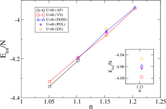
Figure 2: (Color online) Comparison of the energy per particle for different configurations in a $14\times 14$ lattice for different densities $n$. AF stands for antiferromagnetism, VS for in-phase vertical stripes (Fig. 3 (up)), DOM for in-phase antiferromagnetic domains (Fig. 3 (down)), POL for polarons and DS for in-phase diagonal stripes. The inset shows the $U=8t$ and $n=1.15$ region enlarged to appreciate better the difference in the energies.

Figure 3: Configuration for $U=8t$, $t^{\prime}=-0.3t$ and $n=1.15$ in a $24\times 24$ lattice for in-phase vertical stripes -VS- (up) and in-phase antiferromagnetic domains -DOM- (down). The circles and arrows are scaled to the local charge and spin.

To check that the results obtained are robust over the size of the lattice and as in the following section we will use results for a $24\times 24$ lattice we have made a comparison of the energy per particle for different lattice sizes. The results are shown in Table 1. The compared energy per particle are for homogeneous antiferromagnetism (AF) and inhomogeneous in-phase stripes (VS) configurations for two lattice sizes $12\times 12$ and $24\times 24$. The lattice size has been chosen for convenience to fit the inhomogeneous configuration. In the homogeneous case the variation in energy is almost negligible and in the VS case it is appreciable in the fourth decimal digit. Therefore we can trust that the phase diagram will remain for bigger lattice sizes.

Conf.	$E/L(12\times 12)$	$E/L(24\times 24)$
AF	-4.46587799	-4.46587795
VS	-4.04248799	-4.04257066

Table 1: Energy per site in units of $t$ of different configurations for different lattice sizes $12\times 12$ and $24\times 24$ for $U=8t$ and $t^{\prime}=-0.3t$. In the homogeneous solution (AF) at $n=1$ the difference is negligible and for the inhomogeneous solution (VS) at $n=1.16$ it is appreciable in the fourth digit.

Next we compare in-phase with off-phase stripes. We have chosen a different lattice size ($16\times 16$) to fit the off-phase configuration. For the points shown in Fig. 1, off-phase vertical stripes only converge at $n=1.15$ and $U=8t$ as an excited state, though the energy per particle is very similar to the in-phase stripe ($E_{VS}/L=-4.090t$, $E_{STRIPE}/L=-4.083t$). Therefore, within Unrestricted Hartree Fock, in-phase stripes are preferred. Adding fluctuations to the unrestricted Hartree-Fock solution could change this view. Calculations using an exact diagonalization method within the dynamical mean field theoryfleck have shown that solitonic formation contributes to the stability of the off-phase stripes. However we have noticed a clear tendency for in-phase solutions that converge easily and in a wider region of the phase diagram.

IV one-particle properties

The spectral function $A({\bf k},\omega)=-\frac{1}{\pi}\Im G_{ret}({\bf k},\omega)$ is evaluated using the time-dependent Green’s function, which can be calculated numerically. When the spectral function is expressed in terms of the new manybody state by Eq. 3 the following expression is obtaineddagotto

$$A({\bf k},\omega)=\frac{1}{L}Re\Big{[}\sum_{{\bf m},{\bf n},s,\lambda}e^{i({\bf m}-{\bf n}){\bf k}}U_{{\bf n}s,\lambda}U_{{\bf m}s,\lambda}^{\dagger}\delta(\omega-E_{\lambda})\Big{]}.$$ (4)

We represent $A({\bf k},\omega)$ in Fig. 4 with the Fermi level at $\omega=0$, for AF (Fig. 4 up) at $n=1.05$ and for DOM (Fig. 4 down) at $n=1.15$. The spin-charge configuration of DOM is represented in Fig. 3 (down) in a $24\times 24$ lattice for parameters $U=8t$ and $t^{\prime}=-0.3t$. The VS represented in Fig. 3 (up) has a similar spectral density as the DOM. We represent the DOM spectral function instead the VS because this result will give us a coherent quasiparticle component in the $B_{2g}$ Raman response though the Fermi level does not crosses the band in the nodal region. In Fig. 4(a) we observe two well known results, (1) $t^{\prime}$ makes the lower band narrower and the upper band wider. In consequence, it is expected that localization effects become more important when we dope with holes than when we dope with electrons. (2) concerning the ${\bf k}$ dependence for homogeneous antiferromagnetism, at low doping the Fermi level goes to the bottom of the upper band at $(\pi,0)$ as suggested in a rigid band structure. This result is compatible with ARPESshen . For inhomogeneous configurations, Fig. 4(b), we do not longer have the rigid band structure view and the spectral weight is reorganized. Midgap states appear and the spectral weight around $(\pi,\pi)$ in the upper band disappear. The Fermi level is again at the bottom of the upper band at $(\pi,0)$. The midgap states will be more appreciated in the density of states.

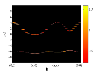
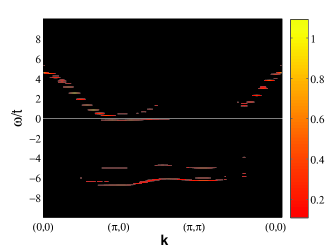
Figure 4: (Color online) $A({\bf k},\omega)$ for different configurations antiferromagnetism at $n=1.05$ (up) and DOM at $n=1.15$ (down). Parameters are $U=8t$, $t^{\prime}=-0.3t$ and $T=0.05t$.

Fig. 5 shows the density of states for the AF and DOM configurations described previously and also for the VS represented in Fig. 3 (up) with a width of $\eta=0.1t$ given to the delta functions. The Fermi level is located at zero energy. We again see for the antiferromagnetic solution (dotted line) the result expected from a rigid band structure, the gap is lower if we compare with the result at half filling (not shown) and the Fermi level is shifted to the upper band. For DOM (solid line) and VS (dashed line) the density of states is very similar. We appreciate the formation of midgap states with almost no gap closing if we compare with the former case at lower doping $n=1.05$. It is interesting to notice in Fig. 5 that for the inhomogeneous solution there is a depression at the Fermi level (it can also be seen in Fig. 4(down)). We do not claim that this corresponds to the pseudogap whose physics needs better approaches, but it is interesting to realize that inhomogeneous solutions can give a feature that it is usually considered as a hallmark of the pseudogap.tremblay

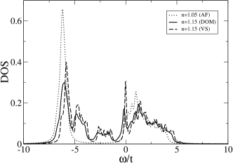
Figure 5: Density of states for homogeneous antiferromagnetism at $n=1.05$ (dotted line), in-phase antiferromagnetic domains DOM (solid line) and in-phase vertical stripes VS (dashed line) at $n=1.15$. Both inhomogeneous configurations present similar density of states with in-gap states and a pseudogap-like feature at the Fermi level. Parameters are $U=8t$, $t^{\prime}=-0.3t$, $T=0.05t$ and $\eta=0.1t$.

Next we discuss further the phase diagram of Fig. 1 with the help of the spectral function (Fig. 4) and the density of states (Fig. 5). A simple argument to understand why the antiferromagnetism is enhanced and dominates the phase diagram of the electron doped case can be given by changing to a Néels state basis. In that basis the $t^{\prime}$ term appears in the diagonal of the Hamiltonian since it represents a hopping within the same sublattice. As such it does not change the antiferromagnetic background. The first electron carrier will go to $(\pi,0)$ (see Fig. 4(up)) with an energy given by $E(\pi,0)=4t^{\prime}+\Delta$ where $\Delta=mU$ and $m$ is the magnetization. As $t^{\prime}<0$ it lowers the energy of the antiferromagnetic solution. A similar argument is given in Ref.tohmaek01 for the electron doped $t-J$ model. This simple argument is reinforced by the study of the stability of the metallic antiferromagnetic solutionstability . In the density of states represented in Fig. 5 can be seen that our antiferromagnetism is also metallic and the whole picture is very similar to what happens in a rigid band model.

Next we discuss the VS at intermediate doping and high $U$. As mentioned when doping with holes we are doping a narrower band and a lower mobility is expected than when doping with electrons. It is not surprising then that inhomogeneities appear at low doping in hole doped and not in the electron doped. However there is a critical density in the electron doped case where inhomogeneities are the preferred configuration as a compromise to minimize the strong Coulomb interaction. In-phase vertical stripes allow more mobility than diagonal stripes and that is why within UHF diagonal are preferred for hole dopedus ; normand and vertical for electron doped.

V Non-resonant Raman response

The differential Raman cross section iscardona

$$\frac{\partial^{2}\sigma}{\partial\omega\partial\Omega}=\frac{\omega_{S}}{\omega_{I}}r_{0}^{2}S_{\gamma\gamma}({\bf q},\omega,\beta),$$ (5)

where $r_{0}=e^{2}/mc^{2}$ is the classical radius of the electron and the generalized dynamic structure factor is

$$\tilde{S}_{\gamma\gamma}({\bf q},\omega,\beta)=\sum_{i,f}\frac{e^{-\beta E_{i}}}{Z}|\langle f|\tilde{\rho}_{\gamma}({\bf q})|i\rangle|^{2}\delta(E_{f}-E_{i}+\hbar\omega).$$ (6)

Here, $\frac{e^{-\beta E_{i}}}{Z}$ is the probability of the initial state in thermodynamic equilibrium. The state $|i\rangle$ is the initial many-body state and $|f\rangle$ is the final many-body state. $\tilde{\rho}({\bf q})$ is an effective charge density given by

$$\tilde{\rho}_{\gamma}({\bf q})=\sum_{\bf k,s}\gamma({\bf k};\omega_{I},\omega_{S})c_{s}^{\dagger}({\bf k+q})c_{s}({\bf k}),$$ (7)

where $s$ is the spin index and $\gamma({\bf k};\omega_{I},\omega_{S})$ is the Raman scattering amplitude. We are interested in the ${\bf q}=0$ case since the momentum transfer by the photon is negligible. The generalized structure factor given by Eq. 6 can be interpreted as the power spectrum of the charge density fluctuations at frequency $\omega$. It is related to the imaginary part of the Raman response function through the fluctuation-dissipation theorem

$$S_{\gamma\gamma}({\bf q},\omega)=-\frac{1}{\pi}[1+n(\omega)]{\rm Im}\chi_{\gamma\gamma}({\bf q},\omega),$$ (8)

where

$$\chi_{\gamma\gamma}({\bf q},\omega)=\int_{0}^{1/T}d\tau e^{-i\omega\tau}\langle T_{\tau}\hat{\rho}(\tau)\rho(0)\rangle.$$ (9)

We will compute the imaginary part of the Raman response by replacing the Hartree-Fock eigenvalues and eigenvectors in the generalized structure factor given by Eq. 6 instead of using the Green’s function machinery in Eq. 9 as it is usually done.

We will follow Ref.devereaux where symmetry is used to classify the scattering amplitude since the different polarizations transform as elements of the point group of the crystal

$$\gamma({\bf k};\omega_{I},\omega_{S})=\sum_{L}\gamma_{L}(\omega_{I},\omega_{S})\Phi_{L}(\bf k),$$ (10)

where $\Phi_{L}(\bf k)$ are the Brillouin zone harmonics (BZH). The use of symmetry arguments instead of the inverse effective mass approximation as it is usually donecardona will allow us to discuss non-resonant Raman response at high energiesdevereaux . In this work we are interested in the $B_{1g}$ and $B_{2g}$ symmetries of the square lattice. The $B_{1g}$ symmetry corresponds to incident and scattered light polarizations aligned along $\hat{x}+\hat{y}$ and $\hat{x}-\hat{y}$, and thus

$$\Phi_{B_{1g}}(\bf k)=\cos(k_{x})-\cos(k_{y})+\cdots,$$ (11)

where the dots stand for higher order BZH. The $B_{2g}$ symmetry corresponds to incident and scattered light polarizations aligned along $\hat{x}$ and $\hat{y}$

$$\Phi_{B_{2g}}(\bf k)=\sin(k_{x})\sin(k_{y})+\cdots,$$ (12)

The $B_{1g}$ signal weights mainly the antinodal quasiparticles and the $B_{2g}$ signal the nodal quasiparticles.

Replacing Eq. 3 in Eq. 7 and Eq. 6 we obtain for the $B_{1g}$ and the $B_{2g}$ Raman expressions

$${\rm Im}\chi_{B_{1g}}(\omega)=\frac{\pi}{L}\sum_{\lambda\neq\lambda^{\prime}}\frac{e^{-\beta E_{\lambda}}}{(1+e^{-\beta E_{\lambda^{\prime}}})(1+e^{-\beta E_{\lambda}})}$$ (13)

$$\delta(\omega+(E_{\lambda}-E_{\lambda^{\prime}}))|\sum_{{\bf j}=(x,y)s}(U_{(x+1,y)s,\lambda}^{\dagger}U_{(x,y)s,\lambda^{\prime}}+h.c)$$

$$-(U_{(x,y+1)s,\lambda}^{\dagger}U_{(x,y)s,\lambda^{\prime}}+h.c)|^{2},$$

$${\rm Im}\chi_{B_{2g}}(\omega)=\frac{\pi}{L}\sum_{\lambda\neq\lambda^{\prime}}\frac{e^{-\beta E_{\lambda}}}{(1+e^{-\beta E_{\lambda^{\prime}}})(1+e^{-\beta E_{\lambda}})}$$

$$\delta(\omega+(E_{\lambda}-E_{\lambda^{\prime}}))|\sum_{{\bf j}=(x,y)s}(U_{(x+1,y-1)s,\lambda}^{\dagger}U_{(x,y)s,\lambda^{\prime}}+h.c)$$

$$-(U_{(x+1,y+1)s,\lambda}^{\dagger}U_{(x,y)s,\lambda^{\prime}}+h.c)|^{2}.$$

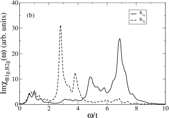
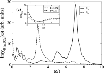
Figure 6: (a) Evolution of the $B_{1g}$ and $B_{2g}$ Raman signal with doping for antiferromagnetism for $U=6t$, $x=0.05$ (solid line) and $x=0.1$ (dashed line). (b) $B_{1g}$ and $B_{2g}$ Raman signal for VS (Fig. 3 (up)) at $U=8t$ and $n=1.15$. (c) $B_{1g}$ and $B_{2g}$ Raman signal for DOM (Fig. 3 (down)) at $U=8t$ and $n=1.15$. In the inset is shown the evolution with temperature of the $B_{2g}$ signal for low frequencies. Parameters are $t^{\prime}=-0.3t$, $T=0.05t$ and $\eta=0.1t$.

Fig. 6 shows the non-resonant Raman response. In experiments for cuprates, the range in frequencies is just up to around $1t$ and at high frequencies the resonant Raman response is unavoidable and it could couple with the non resonant one as has been recently shown with Dynamical mean field theorydevereauxres , but we show the complete range of frequencies to illustrate the physics that comes up from our calculations. We can phenomenologically decompose the Raman response as following: $\chi^{\prime\prime}(\omega)=\chi^{\prime\prime}_{low\omega}+\chi^{\prime\prime}_{incoh}+\chi^{\prime\prime}_{gap}$. The low frequency response is usually fitted as a quasiparticle response $\chi^{\prime\prime}_{QEP}(\omega)=a\frac{\Gamma\omega}{\omega^{2}+\Gamma^{2}}$, in our case $\Gamma=0$ since we did not put any scattering rate as input, and therefore $\chi^{\prime\prime}_{QEP}=0$. But for some cases we find $\chi_{low\omega}\neq 0$ as we will see in the following. $\chi^{\prime\prime}_{gap}$ is formed by the pronounced peak at high energies in both figures and is due to the antiferromagnetic gap. $\chi^{\prime\prime}_{incoh}$ is formed by the rest. In experiments this part is almost a constant continuum background and gave rise to the Marginal Fermi liquid phenomenologymfl . Next we discuss the results. Fig. 6(a) represents the evolution with doping of the $B_{1g}$ and $B_{2g}$ Raman signals for homogeneous antiferromagnetism with parameters $U=6t$, $t^{\prime}=-0.3t$ and dopings $n=1.05$ (solid line) and $n=1.1$ (dashed line). Again a width of $\eta=0.1t$ is given to the delta functions. As expected for homogeneous antiferromagnetism the signal for the $B_{2g}$ channel is negligible and cannot be appreciated in Fig. 6(a) and in the $B_{1g}$ channel, $\chi^{\prime\prime}_{gap}$ is the only appreciable component. We can observe a shift in $\chi^{\prime\prime}_{gap}$ for $n=1.1$ compared with $n=1.05$ reflecting the closing of the gap with increasing doping. That $\chi^{\prime\prime}_{low\omega}$ and the $\chi^{\prime\prime}_{incoh}$ are negligible might be due to the fact that the charge is completely homogeneous for this antiferromagnetism and from Eq. 13 and Eq. V we see that for homogeneous phases is very likely that the Raman matrix elements are zero. We have checked this result with all the homogeneous configurations that we have found with the same null result for $\chi^{\prime\prime}_{low\omega}$ and $\chi^{\prime\prime}_{incoh}$. Fig. 6(b) and (c) represents the $B_{1g}$ and $B_{2g}$ Raman signals for the inhomogeneous solution consisting of VS and DOM at $U=8t$, $t^{\prime}=-0.3t$ and $n=1.15$. In both figures a gap is observed at high frequencies and $\chi^{\prime\prime}_{incoh}$ is no longer zero neither in $B_{1g}$ nor in $B_{2g}$ channels. The gap appears at higher energy in the $B_{1g}$ channel consistent with Fig. 4 (down). The incoherent background comes from the in-gap states in the density of states, see Fig. 5. For VS there is not low-frequency component in any channel but for DOM, the $B_{2g}$ channel has a $\chi^{\prime\prime}_{low\omega}$ component with a quasiparticle-like shape and it is not clear in the $B_{1g}$ channel. We have calculated the evolution with temperature of the Raman signal shown in the inset of Fig. 6(c). The decrease with temperature of the $\chi^{\prime\prime}_{QEP}$ for the $B_{2g}$ channel would have been interpreted as a metallic behavior in experiments. We arrive at two interesting results for the inhomogeneous solution, (1) there is a remarkable incoherent component, and (2) the $B_{2g}$ channel has a quasiparticle-like component for the DOM configuration. We can also find this behavior for higher doping in the VS configuration. This means that the low energy part of the Raman response can arise not only from the real quasiparticle component but also from inhomogeneities. In the last case this quasiparticle-like response has no relation with real quasiparticles since the Fermi level does not cross the nodal region. It might arise because inhomogeneities create an effective Raman scattering rate that can contribute to the low frequency region of the Raman response.

VI Conclusions

We find in-phase inhomogeneities as the lowest energy configurations for strong-coupling limit at intermediate dopings. These results are interesting because the doping region where inhomogeneities are found signals another quantitative asymmetry for hole and electron doped cuprates. Inhomogeneities are present at very low doping for hole doped cuprates and only at intermediate to high doping for electron doped. This region of intermediate doping is precisely the region where the antiferromagnetic phase is suppressed ($n\approx 1.5$). The result agrees with a recent theoretical proposal of phase separation for this range of parametersarrigoni . It is also interesting to notice that we need to be in the strong coupling limit to find the inhomogeneities, since they are formed to minimize the strong on-site interaction. Experimentally electron doped cuprates seem to be in the strong coupling limit as much as hole doped cupratesmillis but there is a theoretical debate on whether or not strong coupling is necessary to understand electron dopedhanke . In-phase inhomogeneities are compatible with experiments of inelastic neutron scattering and thermal conductivityando . However to fully address this issue quantum fluctuations should be taken into account since they can favor off-phase stripesfleck .

The inhomogeneities give rise to midgap states in the density of states as found by ARPESarmitage though at strong coupling it is not possible to obtain a quasiparticle signal in the nodal region. for what better techniques taking into account quantum fluctuations should be used. For the non-resonant Raman response the in-phase inhomogeneities give an incoherent background at low and intermediate frequencies. For the DOM configuration (Fig. 3 (down)) the $B_{2g}$ signal have stronger quasiparticle-like component than the $B_{1g}$ signal though the Fermi level does not cross the nodal region. This is an example where two particle properties can not be inferred from one particle properties. It would be interesting to check if the quasiparticle component of the $B_{2g}$ Raman response is different from zero in the region where ARPES does not show quasiparticle weight in the nodal region.

- (1) T. R. Thurston, M. Matsuda, K. Kakurai, K. Yamada, Y. Endoh, R. J. Birgeneau, P. M. Gehring, Y. Hidaka, M. A. Kastner, T. Murakami, and G. Shirane, Phys. Rev. Lett. 65, 263 (1990).
- (2) S.A. Kivelson, I.P. Bindloss, E. Fradkin, V. Oganesyan, J.M. Tranquada, A. Kapitulnik, and C. Howald, Rev. Mod. Phys. 75, 1201 (2003).
- (3) J. M. Tranquada, cond-mat/0512115 (2005) to appear as a chapter in Treatise of High Temperature Superconductivity by J. Robert Schrieffer, to be published.
- (4) S.D. Wilson, S. Li, H. Woo, P. Dai, H.A. Mook, C.D. Frost, S. Komiya, Y. Ando, Phys. Rev. Lett. 96, 157001 (2006); K. Yamada, K. Kurahashi, T. Uefuji, M. Fujita, S. Park, S.-H. Lee and Y. Endoh, Phys. Rev. Lett. 90, 137004 (2003).
- (5) T. Tohyama and S. Maekawa Phys. Rev. B 49, 3596 (1994).
- (6) R.J. Gooding, K.J.E. Vos and P.W. Leung, Phys. Rev. B 50, 12866 (1994).
- (7) D. Duffy and A. Moreo, Phys. Rev. B 52, 15607 (1995).
- (8) J-X. Li, J. Zhang and J. Luo, Phys. Rev. B 68, 224503 (2003).
- (9) M. Raczkowski, A. M. Oleś and R. Frésard, Low. Temp. Phys. 32, 411 (2006).
- (10) X. F. Sun, Y. Kurita, T. Suzuki, Seiki Komiya, and Yoichi Ando, Phys. Rev. Lett. 92, 047001 (2004); P. Dai, H. J. Kang, H. A. Mook, M. Matsuura, J. W. Lynn, Y. Kurita, S. Komiya, Y. Ando, Phys. Rev. B 71, 100502(R) (2005).
- (11) F. Zamborszky, G. Wu, J. Shinagawa, W. Yu, H. Balci, R.L Greene, W.G. Clark and S.E. Brown, Phys. Rev. Lett. 92, 47003 (2004); O.N. Bakharev, I.M. Abu-Shiekah, H.B. Brom, A.A. Nugroho, I.P. McCulloch, and J. Zaanen, ibid 93, 37002 (2004). L. P. Gor’kov and G. B.Teitel’baum, Solid State Communications 137, 288 (2006).
- (12) L. Alff, Y. Krockenberger, B. Welter, M. Schonecke, R. Gross, D. Manske and M. Naito, Nature 422, 698 (2003).
- (13) W.P. Su, Phys. Rev. B 37, 9904 (1988); D. Poilblanc and T.M. Rice, Phys. Rev. B 39, 9749 (1989); J. Zaanen and O. Gunnarsson,Phys. Rev. B 40, 7391 (1989).
- (14) S. Caprara, C. Di Castro, M. Grilli, and D. Suppa, Phys. Rev. Lett. 95, 117004 (2005).
- (15) A. Sadori and M. Grilli, Phys. Rev. Lett 84, 5375 (2000).
- (16) A. Macridin, M. Jarrell, T. Maier and P.R.C. Kent, cond-mat/0509166 (2005); A.-M.S. Tremblay, B. Kyung and D. Sénéchal, Fizika Nizkikh Temperatur (Low Temperature Physics), 32 561 (2006) (cond-mat/0511334).
- (17) C.Dahnken, M. Potthoff, E. Arrigoni and W. Hanke, cond-mat/0504618.
- (18) Q. Yuan, Y. Chen, T.K. Lee and C. S. Ting,Phys. Rev. B 69, 214523 (2004); Q. Yuan, F. Yuan and C. S. Ting,Phys. Rev. B 72, 54504 (2005).
- (19) A. Macridin, M. Jarrell, Th. Maier, G.A. Sawatzky Phys. Rev. B 71, 134527 (2005)
- (20) B. Valenzuela, M.A.H. Vozmediano and F. Guinea, Phys. Rev. B 62, 11312 (2000).
- (21) B. Normand and A.P. Kampf, Phys. Rev. B 64, 024521 (2001).
- (22) T. Tohyama, Phys. Rev. B 70, 174517 (2004) and references therein.
- (23) P.W. Leung, Phys. Rev. B 73, 75104 (2006).
- (24) Z.B. Huang, H.Q. Lin and J.E. Gubernatis, Phys. Rev. B 64, 205101 (2001).
- (25) Y. Onose, Y. Taguchi, K. Ishizaka and Y. Tokura, Phys. Rev. B 69, 24504 (2004) and references therein.
- (26) M. Aichhorn and E. Arrigoni, cond-mat/0502047 (2005) accepted in Europhysics Letters; M. Aichhorn, E. Arrigoni, M. Potthoff and W. Hanke, cond-mat/0511460 (2005).
- (27) N. P. Armitage, F. Ronning, D. H. Lu, C. Kim, A. Damascelli, K. M. Shen, D. L. Feng, H. Eisaki, Z.-X. Shen, P. K. Mang, N. Kaneko, M. Greven, Y. Onose, Y. Taguchi, Y. Tokura, Phys. Rev. Lett. 88, 257001 (2002).
- (28) C. Kusko, R.S. Markiewicz, M. Lindroos and A. Bansil, Phys. Rev. B 66, 140513(R) (2002).
- (29) H. Kusunose and T.M. Rice, Phys. Rev. Lett. 91, 186407 (2003).
- (30) M. M. Qazilbash, B. S. Dennis, C. A. Kendziora, H. Balci, R. L. Greene, G. Blumberg, cond-mat/0501362; M.M. Qazilbash, A. Koitzsch, B.S. Dennis, A. Gozar, H. Balci, C.A. Kendziora, R.L. Greene, and G. Blumberg, Phys. Rev. B 72, 214510 (2005).
- (31) A. J. Millis, A. Zimmers, R. P. S. M. Lobo, N. Bontemps, C.C. Homes, Phys. Rev. B 72, 224517 (2005).
- (32) X.J. Zhou, T. Yoshida, D.-H. Lee, W. L. Yang, V. Brouet, F. Zhou, W. X. Ti, J. W. Xiong, Z. X. Zhao, T. Sasagawa, T. Kakeshita, H. Eisaki, S. Uchida, A. Fujimori, Z. Hussain, and Z.-X. Shen, Phys. Rev. Lett. 92, 187001 (2004).
- (33) J.A. Vergés, E. Louis, P.S. Lomdahl, F. Guinea and A.R. Bishop, Phys. Rev. B 43, 6099 (1991).
- (34) M. Fleck , A.I. Lichtenstein, A.M. Oleś Phys. Rev. B 64, 134528 (2001).
- (35) The development of the Green function can be followed in detail in the book by Dagotto: Nanoscale phase separation and colossal magnetoresistance : the physics of manganites and related compounds, chapter 7. Section 7.5. I have applied the same ideas to find the Raman response with the unrestricted Hartree Fock solutions.
- (36) A. Damascelli, Z. Hussain, and Z.-X. Shen Rev. Mod. Phys. 75, 473 (2003).
- (37) A. Singh and H. Ghosh, Phys. Rev. B 65, 134414 (2002).
- (38) T. Tohyama and S. Maekawa, Phys. Rev. B 64, 212505 (2001).
- (39) M. Cardona, editor, Light scattering in solids 1, 2nd edition (Springer-Verlag, Berlin, 1983), chap. Electronic Raman scattering by M.V. Klein.
- (40) T.P. Devereaux and A.P. Kampf, Phys. Rev. B 59, 6411 (1999).
- (41) A.M. Shvaika, O.Vorobyov, J.K. Freericks, and T.P. Devereaux, Phys. Rev. Lett 93, 137402 (2004); A.M. Shvaika, O.Vorobyov, J.K. Freericks, and T.P. Devereaux, Phys. Rev. B 71, 45120 (2005).
- (42) C.M. Varma, P.B. Littlewood, S. Schmitt-Rink, E. Abrahams and A.E. Ruckenstein, Phys.Rev.Lett 63, 1996 (1989).