Parametric instability of homogeneous precession of spin in the superfluid ${}^{3}He-B$

Abstract

Stability of homogeneous precession of spin due to parametric excitation of spin waves is considered as the explanation of the ”catastrophic relaxation”, that is observed in the superfluid ${}^{3}He-B$. It is shown, that at sufficiently low temperatures homogeneous precession of spin becomes unstable (Suhl instability). At zero temperature increments of growth for all spin wave modes are found. Estimation of the temperature of transition to the unstable state is made.

1. The use of pulsed NMR is based on the investigation of homogeneous precession of spin in a constant magnetic field. Spin precession induces the free induction signal (FIS), which is registered in the induction coil. Precession of spin in the superfluid B-phase of³He has its specifics. At temperatures $T\geq 0,4T_{c}$, where $T_{c}$ is the temperature of superfluid transition, FIS exists anomalously long – many times longer than the time of dephasing of spin due to a residual inhomogeneity of d.c. field. At $T\sim 0,4T_{c}$ occurs transition into the other regime, when on the contrary FIS disappears quickly. This fast decay of precession was first observed in ref. [1] and since that is referred as catastrophic relaxation. While anomalously long FIS was explained a long time ago, even a qualitative explanation for the catastrophic relaxation is missing. The decay of homogeneous precession was demonstrated by numeric simulation of equations of spin dynamics [2]. The simulation was made in the restricted geometry and the authors of simulation attribute the main role in the destruction of precession to the walls, i.e. they consider the mechanism of destruction to be surface.

In the present paper the explanation of catastrophic relaxation is suggested, which is based on a bulk effect. It is the instability of homogeneous precession with respect to decay into parametrically excited spin waves with opposite wave vectors (Suhl instability [3]).

Fast decay of precession was also observed in the $uudd$-phase of solid ³He and it was explained by the onset of Suhl instability [4]. However, the quantitative interpretation of the results, concerning instability of precession in the cited work is based on the modification of theory Ref. [5], developed for the continuous NMR and which is therefore applicable only for small tipping angles. In our analysis this restriction is not used and it can be applied for the arbitrary angles between spin and magnetic field.

2. In order to describe motion of spin we use expression of Hamiltonian of Leggett, which is written in terms of Euler angles $\alpha$, $\beta$, $\Phi=\alpha+\gamma$ (z-axis is oriented opposite to the direction of d.c. magnetic field $\bf H_{0}$) as coordinates and canonically conjugated momenta $P=S_{z}-S_{\zeta}$, $S_{\beta}$, $S_{\zeta}$, where $S_{z}$ — is projection of spin onto z-axis, $S_{\zeta}$ —its projection onto axis $\zeta=\hat{R}\hat{\emph{z}}$ and $S_{\beta}$ — is projection on the line of nodes (see for details [6]). We choose units of measurement so that $\chi=g=1$, where $\chi$ — is magnetic susceptibility per unit volume of ${}^{3}He-B$, and g — is the gyromagnetic ratio for nuclei of ${}^{3}He$; after that spin has dimensionality of frequency and energy of the frequency squared. Using variable and units mentioned above one can write the Hamiltonian in the form:

$$H=\frac{1}{1+\cos{\beta}}\{S_{\zeta}^{2}+PS_{\zeta}+\frac{P^{2}}{2(1-\cos{\beta})}\}+\frac{1}{2}S_{\beta}^{2}+F_{\nabla}-\omega_{L}(P+S_{\zeta})+U_{D}(\beta,\Phi),$$ (1)

where $\omega_{L}$ - is Larmor frequency corresponding to the d.c. magnetic field, $F_{\nabla}$ - gradient energy,$U_{D}(\beta,\Phi)$ - dipole energy. $U_{D}$ for ${}^{3}He-B$ depends only on two variables $\beta$ and $\Phi$, that justifies the choice of $\Phi$ as a variable, when the dipole energy is essential. Gradient energy for ${}^{3}He-B$ can be written as:

$$F_{\nabla}=\frac{1}{2}[c_{\|}^{2}\delta_{ik}\delta_{\xi\eta}-(c_{\|}^{2}-c_{\bot}^{2})(\delta_{i\xi}\delta_{k\eta}+\delta_{i\eta}\delta_{k\xi})]\omega_{i\xi}\omega_{k\eta},$$ (2)

where

$$\omega_{1\xi}=-\alpha_{,\xi}\sin\beta\cos\gamma+\beta_{,\xi}\sin\gamma,$$

$$\omega_{2\xi}=\alpha_{,\xi}\sin\beta\sin\gamma+\beta_{,\xi}\cos\gamma,~{}~{}$$ (3)

$$\omega_{3\xi}=\alpha_{,\xi}\cos\beta+\gamma_{,\xi},{~{}~{}~{}~{}~{}~{}~{}~{}~{}~{}~{}~{}~{}~{}~{}}$$

$\alpha_{,\xi}=\frac{\partial\alpha}{\partial x_{\xi}}$ etc.,$c_{\|}^{2}{}\mbox{ }c_{\bot}^{2}$ — are squared velocities of two types of spin waves (”longitudinal” and ”transverse”). In what follows we choose units in such a way as to $c_{\|}^{2}=1$, then wave vectors entering the equation will also have dimensionality of frequency. Equations of motion, that are generated by Hamiltonian have the form:

$$\frac{\partial\alpha}{\partial t}=\frac{\partial H}{\partial P},{~{}~{}~{}}\frac{\partial P}{\partial t}=-\frac{\partial H}{\partial\alpha}+\frac{\partial}{\partial x_{\xi}}\frac{\partial H}{\partial\alpha_{,\xi}},{~{}~{}}$$ (4)

etc.

System of equation (4) has spatially uniform stationary solution describing precession of spin in the stationary magnetic field at $0\leq\beta<\theta_{0}=\arccos(-\frac{1}{4})$ :

$$\alpha=\omega_{L}t+\alpha_{0},{~{}~{}}\gamma=-\omega_{L}t+\Phi^{0}-\alpha_{0},$$

$$P^{(0)}=\omega_{L}(\cos\beta-1),{~{}~{}}S_{\beta}^{(0)}=0,{~{}~{}}S_{z}^{(0)}=\omega_{L}\cos\beta,$$ (5)

$$\cos\Phi^{(0)}=(\frac{1}{2}-\cos\beta^{(0)})/(1+\cos\beta^{(0)}).\$$

It is convenient to introduce $\psi=\alpha+\omega_{L}t$ instead of $\alpha$ and at the same time to transform the Hamiltonian $\tilde{H}=H+\omega_{L}P$, so that $\frac{\partial\psi}{\partial t}=0$.

Let us now obtain equations for the small deviations from the stationary solution:

$$\delta\psi(\textbf{r},t)=\psi-\psi^{(0)},$$ (6)

etc.

In zeroth approximation on the small deviations the gradient energy has three groups of terms: ”stationary” - with time-independent coefficients, and two ”oscillating”, corresponding to Larmor and doubled Larmor frequencies. Without the loss of generality we consider perturbations propagating in $yz$ plane:

$$F_{\nabla st}=\frac{1}{2}[\delta\psi_{,y}^{2}[1-\mu\sin^{2}{\beta^{(0)}}]+(1-\mu)\delta\beta_{,y}^{2}+\delta\gamma_{,y}^{2}+2\delta\psi_{,y}\delta\gamma_{,y}\cos\beta^{(0)}+$$

$$\delta\psi_{,z}^{2}[1-2\mu\cos^{2}{\beta^{(0)}}]+\delta\beta_{,z}^{2}+\delta\gamma_{,z}^{2}(1-2\mu)+2\delta\psi_{,z}\delta\gamma_{,z}\cos\beta^{(0)}(1-2\mu)],$$ (7)

$$F_{\nabla osc1}=-\mu[\delta\psi_{,y}\delta\psi_{,z}\sin 2\beta^{(0)}\sin\omega_{L}t+$$

$$+(\delta\psi_{,y}\delta\gamma_{,z}+\delta\psi_{,z}\delta\gamma_{,y})\sin\beta^{(0)}\sin\omega_{L}t+(\delta\psi_{,y}\delta\beta_{,z}+\delta\psi_{,z}\delta\beta_{,y})\cos\beta^{(0)}\cos\omega_{L}t+$$

$$+(\delta\beta_{,y}\delta\gamma_{,z}+\delta\beta_{,z}\delta\gamma_{,y})\cos\omega_{L}t],$$ (8)

$$F_{\nabla osc2}=-\frac{\mu}{2}[\sin^{2}{\beta^{(0)}}\delta\psi_{,y}^{2}\cos{2\omega_{L}t}-\delta\beta_{,y}^{2}\cos{2\omega_{L}t}+$$

$$+\sin\beta^{(0)}\delta\psi_{,y}\delta\beta_{,y}\sin{2\omega_{L}t}].$$ (9)

Oscillating terms are proportional to $\mu=1-c_{\bot}^{2}/c_{\|}^{2}$. We assume that $\mu$ is small, and consider oscillating terms in the equations of motion as small perturbations. Actually $\mu$ is not very small ($\mu\approx 1/4$ in a vicinity of $T_{c}$), however, this approximation gives satisfactory results. More precise criteria of application of such approximation will be formulated in a process of solution.

In order to use the theory of perturbation we write linearized system of equations of motion in the form:

$$\frac{d\mathbf{X}}{dt}=\left(\hat{M}_{0}+\hat{V}(t)\right)\mathbf{X},$$ (10)

where

$$\textbf{X}=\left(\begin{array}[]{c}\delta\psi\\ \delta\beta\\ \delta\Phi\\ \delta S_{z}\\ \delta S_{\beta}\\ \delta P\end{array}\right).$$

Matrix operator $\hat{M}_{0}$ includes all time-independent terms, and oscillating terms are collected in matrix operator $\hat{V}(t)$, which is proportional to $\mu$ and therefore is considered as a perturbation. Equation of zero order approximation on perturbation:

$$\frac{d\mathbf{X}}{dt}=\hat{M}_{0}\mathbf{X},$$ (11)

gives us dispersion laws for the three branches of spin waves:

$$\begin{array}[]{lc}\omega_{1}^{2}=k^{2},\\ \omega_{2}^{2}=\frac{1}{2}\omega_{L}^{2}+k^{2}-\frac{1}{2}\omega_{L}\sqrt{\omega_{L}^{2}+4k^{2}},\\ \omega_{3}^{2}=\frac{1}{2}\omega_{L}^{2}+k^{2}+\frac{1}{2}\omega_{L}\sqrt{\omega_{L}^{2}+4k^{2}}\end{array}$$

and eigenvectors, corresponding to each oscillation branch $\textbf{X}_{i}(k),~{}i=1,2,3$. Recall that we are speaking about the spin waves propagating against the background of homogeneous precession, so the mentioned oscillations of spin are different from the usual spin waves, which are created by small deviation from equilibrium orientation. It is assumed here that $\omega_{L}\gg\Omega$, where $\Omega$ is the frequency of longitudinal oscillations.

Solution of the system (11) is given by:

$$\textbf{X}(t,k,y,z)=\sum^{3}_{i=1}\{a_{i-}\textbf{X}_{i}(k)\exp(-i\omega_{i}(k)t+i\textbf{k}\textbf{r})$$

$$a_{i+}\textbf{X}_{i}^{*}(k)\exp(i\omega_{i}(k)t+i\textbf{k}\textbf{r})+$$

$$a_{i-}^{*}\textbf{X}_{i}^{*}(k)\exp(i\omega_{i}(k)t-i\textbf{k}\textbf{r})+$$

$$a_{i+}^{*}\textbf{X}_{i}(k)\exp(-i\omega_{i}(k)t-i\textbf{k}\textbf{r})\},$$ (13)

where $a_{i}$ - are constant coefficients, $\textbf{k}=(k_{y},k_{z})$ and $\textbf{r}=(y,z)$ are 2D vectors. When $\hat{V}(t)$ is taken into account $\textbf{X}(t,k,y,z)$, given by equation (Parametric instability of homogeneous precession of spin in the superfluid ${}^{3}He-B$), does not satisfy the equation of motion (10). The first order approximation on $\hat{V}$ can be obtained by the method of averaging of the classical mechanics. Substituting zero order approximation (Parametric instability of homogeneous precession of spin in the superfluid ${}^{3}He-B$) into formulas (Parametric instability of homogeneous precession of spin in the superfluid ${}^{3}He-B$),(Parametric instability of homogeneous precession of spin in the superfluid ${}^{3}He-B$) we can see that terms of the first order on $\mu$ will not vanish after time averaging only if there are resonance relations between $\omega_{L}$ and eigenfrequencies $\omega_{i}(k)$: $\omega_{i}(k)=\omega_{L}$ and $\omega_{i}(k)=\omega_{L}/2$. As it is seen from equations (12) for all branches of spin waves there exist $k$ which are satisfies such resonance conditions. Vicinities of these wave vectors are ”dangerous” for the appearance of instability. From the same formulas it follows that for the different branches resonance conditions are satisfied with different values of wave vectors, and therefore each branch can be considered independently. To find solution nearby the resonance frequencies we will use the standard procedure, when solution in the main approximation is sought in a form:

$$\textbf{X}^{(l)}(t,k^{{}^{\prime}},y,z)=a_{i-}(t)\textbf{X}_{i}(k^{{}^{\prime}})\exp(-i\omega_{R}^{(l)}t+i\textbf{k}^{{}^{\prime}}\textbf{r})+$$

$$a_{i+}(t)\textbf{X}_{i}^{*}(k^{{}^{\prime}})\exp(i\omega_{R}^{(l)}t+i\textbf{k}^{{}^{\prime}}\textbf{r})+$$

$$a_{i-}^{*}(t)\textbf{X}_{i}^{*}(k^{{}^{\prime}})\exp(i\omega_{R}^{(l)}t-i\textbf{k}^{{}^{\prime}}\textbf{r})+$$

$$a_{i+}^{*}(t)\textbf{X}_{i}(k^{{}^{\prime}})\exp(-i\omega_{R}^{(l)}t-i\textbf{k}^{{}^{\prime}}\textbf{r}),$$ (14)

$l=1,2$, where $\omega_{R}^{(l)}$, - is one of the resonance frequencies ($\omega_{R}^{(1)}=\omega_{L}/2$, $\omega_{R}^{(2)}=\omega_{L}$, we will suppress index $l$ in the nearest formulas for brevity),$k^{{}^{\prime}}$- is wave vector nearby resonance frequency for the i-mode, $a_{i}(t)$ - are ”slowly” varying functions of time, i.e. $\dot{a}_{\pm}\sim\mu a_{\pm}$. Terms, that have frequencies differing from $\omega_{R}$ on integer multiple of $2\omega_{L}$ — $3\omega_{R},5\omega_{R},7\omega_{R}$ appear in the next orders on $\mu$.

Substitution of solution (Parametric instability of homogeneous precession of spin in the superfluid ${}^{3}He-B$) into system (10) gives us:

$$\textbf{X}_{a}+\textbf{X}_{\omega_{R}}=\hat{M}(k^{{}^{\prime}})\textbf{X}(t,k^{{}^{\prime}},y,z)+\hat{V}(\textbf{k}^{{}^{\prime}},t)\textbf{X}(t,k^{{}^{\prime}},y,z),$$ (15)

where

$$\textbf{X}_{a}=\dot{a}_{i-}(t)\textbf{X}_{i}(k^{{}^{\prime}})\exp(-i\omega_{R}t+i\textbf{k}^{{}^{\prime}}\textbf{r})+$$

$$\dot{a}_{i+}(t)\textbf{X}_{i}^{*}(k^{{}^{\prime}})\exp(i\omega_{R}t+i\textbf{k}^{{}^{\prime}}\textbf{r})+$$

$$\dot{a}_{i-}^{*}(t)\textbf{X}_{i}^{*}(k^{{}^{\prime}})\exp(i\omega_{R}t-i\textbf{k}^{{}^{\prime}}\textbf{r})+$$

$$\dot{a}_{i+}^{*}(t)\textbf{X}_{i}(k^{{}^{\prime}})\exp(-i\omega_{R}t-i\textbf{k}^{{}^{\prime}}\textbf{r}),$$ (16)

$$\textbf{X}_{\omega_{R}}=-i\omega_{R}a_{i-}(t)\textbf{X}_{i}(k^{{}^{\prime}})\exp(-i\omega_{R}t+i\textbf{k}^{{}^{\prime}}\textbf{r})+$$

$$i\omega_{R}a_{i+}(t)\textbf{X}_{i}^{*}(k^{{}^{\prime}})\exp(i\omega_{R}t+i\textbf{k}^{{}^{\prime}}\textbf{r})+$$

$$i\omega_{R}a_{i-}^{*}(t)\textbf{X}_{i}^{*}(k^{{}^{\prime}})\exp(i\omega_{R}t-i\textbf{k}^{{}^{\prime}}\textbf{r})+$$

$$-i\omega_{R}a_{i+}^{*}(t)\textbf{X}_{i}(k^{{}^{\prime}})\exp(-i\omega_{R}t-i\textbf{k}^{{}^{\prime}}\textbf{r}).$$ (17)

Taking into account that $\textbf{X}_{i}(k^{{}^{\prime}})$ and $\textbf{X}^{*}_{i}(k^{{}^{\prime}})$ are eigenvectors of $\hat{M}$, corresponding to the frequencies $\omega_{i}(k^{{}^{\prime}})$ and $-\omega_{i}(k^{{}^{\prime}})$ one can rewrite equation (15) as:

$$\textbf{X}_{a}+\textbf{X}_{\omega_{R}}-\textbf{X}_{\omega_{k}}=\hat{V}(\textbf{k}^{{}^{\prime}},t)\textbf{X}(t,k^{{}^{\prime}},y,z),$$ (18)

or

$$\textbf{X}_{a}-\frac{\varepsilon(k^{{}^{\prime}})}{\omega_{R}}\textbf{X}_{\omega_{R}}=\hat{V}(\textbf{k}^{{}^{\prime}},t)\textbf{X}(t,k^{{}^{\prime}},y,z),$$ (19)

where $\varepsilon(k^{{}^{\prime}})=\omega(k^{{}^{\prime}})-\omega_{R}$.

Let us multiple the last equation by $\exp(-i\textbf{k}^{{}^{\prime}}\textbf{r})$ and take integral over volume. As the result $a_{i-}^{*}$ and $a_{i+}^{*}$ vanish. Expressing cosines and sines in terms of exponents:

$$\textbf{X}_{a}^{(l)}-\frac{\varepsilon^{(l)}(k^{{}^{\prime}})}{\omega_{R}^{(l)}}\textbf{X}^{(l)}_{\omega_{R}^{(l)}}=(\hat{V}^{(1)}_{+}(\textbf{k}^{{}^{\prime}})\exp(2i\omega_{R}^{(1)}t)+\hat{V}^{(1)}_{-}(\textbf{k}^{{}^{\prime}})\exp(-2i\omega_{R}^{(1)}t)+$$

$$+\hat{V}^{(2)}_{+}(\textbf{k}^{{}^{\prime}})\exp(2i\omega_{R}^{(2)}t)+\hat{V}^{(2)}_{-}(\textbf{k}^{{}^{\prime}})\exp(-2i\omega_{R}^{(2)}t))\mathbf{X}^{(l)}(t),$$ (20)

one obtains the sum of terms with different powers of exponents. Since $V(t)$ contains cosines and sines of $2\omega_{R}^{(l)}t$, coefficients $a_{i-}(t)$ and $a_{i+}(t)$ are related by exponents with the same powers $\pm i\omega_{R}^{(l)}t$. The resulting equations are multiplied by $\exp(\pm i\omega_{R}^{(l)}t)$ and averaged over rapid oscillations. Finally, after making projection of equations on eigenvector of i-mode one obtains system of two differential equations of first order which relates $a_{i-}(t)$ and $a_{i+}(t)$:

$$\dot{a}_{i+}(t)-i\varepsilon^{(l)}(k^{{}^{\prime}}){a}_{i+}(t)=\frac{<\textbf{X}^{*}_{i}\hat{V}^{(l)}_{-}(\textbf{k}^{{}^{\prime}})\textbf{X}^{*}_{i}>}{|\textbf{X}_{i}|^{2}}a_{i-}(t),$$ (21)

$$\dot{a}_{i-}(t)+i\varepsilon^{(l)}(k^{{}^{\prime}}){a}_{i-}(t)=\frac{<\textbf{X}_{i}\hat{V}^{(l)}_{+}(\textbf{k}^{{}^{\prime}})\textbf{X}_{i}>}{|\textbf{X}_{i}|^{2}}a_{i+}(t).$$ (22)

System (21) has solution proportional to $\exp{(\lambda^{(l)}t)}$, where $\lambda^{(l)}$ is defined by:

$$\lambda^{(l)}_{1,2}=\pm\frac{1}{2}\left(\frac{\displaystyle<\textbf{X}_{i}\displaystyle\hat{V}^{(l)}_{+}(\textbf{k}^{{}^{\prime}})\textbf{X}_{i}>\displaystyle<\textbf{X}_{i}^{*}\displaystyle\hat{V}^{(l)}_{-}(\textbf{k}^{{}^{\prime}})\textbf{X}_{i}^{*}>}{\displaystyle|\textbf{X}_{i}\mid^{4}}-[\varepsilon^{(l)}(k^{{}^{\prime}})]^{2}\right)^{\frac{1}{2}}.$$ (23)

Resonance corresponds to the value of $k^{{}^{\prime}}$, when $\varepsilon^{(l)}(k^{{}^{\prime}})=0$. In a region of $k^{{}^{\prime}}$ close to resonance expression in the brackets is positive. Then one of the values of $\lambda^{(l)}$ corresponds to the growth of amplitude of oscillations, i.e. development of instability begins.

3. Let us consider all possible cases of resonances. For each mode we will write: law of dispersion, eigenvector of this oscillation and increment, which is obtained on the condition of resonance.

First mode. Law of dispersion:

$$\omega_{1}^{2}=k^{2}.$$ (24)

Eigenvector:

$$X_{1-}(k)=\left(\begin{array}[]{c}0\\ 0\\ 1\\ \displaystyle-i\omega_{1}(k)\cos\beta\\ 0\\ \displaystyle i\omega_{1}(k)(1-\cos\beta)\end{array}\right)$$

Resonance at the frequency $\frac{\omega_{L}}{2}$:

$$k^{{}^{\prime}}=\pm\frac{\omega_{L}}{2}.$$ (25)

Increment of growth:

$$\lambda_{1}^{(1)}=\mu\frac{\omega_{L}}{4}\cdot\frac{\sin\beta|1-2\cos\beta|}{2\cos^{2}\beta-2\cos\beta+5}\cdot\sin 2\delta,$$ (26)

where $\delta$ - is the angle between direction of the wave vector and z-axis. Maximum increment corresponds to the direction:

$$\delta_{1}^{(0)}=\frac{\pi}{4}.$$ (27)

As it is seen from (26) increment vanishes in the case of wave vector directed along y-axis.

Resonance at the frequency $\omega_{L}$:

$$k^{{}^{\prime}}=\pm\omega_{L}.$$ (28)

In zeroth order approximation on dipole frequency we have:

$$\lambda_{1}^{(2)}=0.$$ (29)

Finite increment appears when the dipole terms are taken into account in the equations of motion. In this case resonance condition is satisfied by the wave vector:

$$k^{{}^{\prime}}=\omega_{L}-\frac{1}{10}(1+4\cos\beta)\frac{\Omega^{2}}{\omega_{L}},$$ (30)

and eigenvector has corrections of the order of $\Omega^{2}/\omega_{L}^{2}$. With these corrections the increment will be equal to:

$$\lambda_{1}^{{}^{\prime}(2)}=\frac{\mu}{5}\frac{\Omega^{2}}{\omega_{L}}\sin^{2}{\beta}\frac{(1+4\cos\beta)^{1/2}}{(1+\cos\beta)^{1/2}}|1-2\cos\beta|\frac{\sin^{2}\delta}{2+2\cos^{2}{\beta}-2\cos\beta}$$ (31)

Maximum increment corresponds to the direction:

$$\delta_{1}^{{}^{\prime}(0)}=\frac{\pi}{2}.$$ (32)

Second mode. Law of dispersion:

$$\omega_{2}^{2}=\frac{1}{2}\omega_{L}^{2}+k^{2}-\frac{1}{2}\omega_{L}\sqrt{\omega_{L}^{2}+4k^{2}}.$$ (33)

Eigenvector:

$$X_{2-}=\left(\begin{array}[]{c}1\\ i\sin\beta\cdot(\displaystyle\frac{k^{2}}{\omega\cdot\omega_{2}(k)}-\frac{\omega_{2}(k)}{\omega})\\ 1-\cos\beta\\ \displaystyle-\displaystyle\frac{k^{2}}{\omega_{2}(k)}(\sin^{2}\beta)\\ i\sin\beta\cdot(\displaystyle\frac{k^{2}}{\omega}-\frac{\omega_{2}^{2}(k)}{\omega})\\ -\displaystyle\frac{k^{2}}{\omega_{2}(k)}(\sin^{2}\beta)\end{array}\right)$$

Resonance at the frequency $\frac{\omega_{L}}{2}$:

$$k^{{}^{\prime}}=\pm\frac{\sqrt{3}\omega_{L}}{2}.$$ (34)

Increment of growth (to zero order approximation on dipole energy)

$$\lambda_{2}^{(1)}=0.$$ (35)

Resonance at the frequency $\omega_{L}$ (taking into account dipole energy):

$$k^{{}^{\prime}}=\sqrt{2}\omega_{L}-\frac{2}{15}(1-\cos\beta)\frac{\Omega^{2}}{\omega_{L}}.$$ (36)

Increment:

$$\lambda_{2}^{{}^{\prime}(2)}=\frac{2\mu}{5}\frac{\Omega^{2}}{\omega_{L}}\sin^{2}{\beta}(1-\cos\beta)|1-4\sin^{2}{\beta}|\frac{\sin^{2}\delta}{12-2\cos\beta-17\cos^{2}{\beta}+8\cos^{4}{\beta}},$$ (37)

has its maximum for $\delta_{2}^{{}^{\prime}(0)}=\pi/2.$

Third mode. Law of dispersion:

$$\omega_{3}^{2}=\frac{1}{2}\omega_{L}^{2}+k^{2}+\frac{1}{2}\omega_{L}\sqrt{\omega_{L}^{2}+4k^{2}}.$$ (38)

Resonance at the frequency $\frac{\omega_{L}}{2}$ is not possible because the frequency of this mode is larger than $\omega_{L}$ for all $k$. Resonance at the frequency $\omega_{L}$ is also not possible because near $k=0$ $\lambda$ is imaginary.

As it is seen from the Fig. (1) there exists positive increment at least for one of the modes of oscillations for all tipping angles. The main role plays maximum increment that is found for the first mode in the case of resonance frequency $\omega_{L}/2$.

4. The obtained results are correct at $T=0$. At a finite temperature spin waves damp. This leads to appearance of temperature threshold of instability. We can take into account small damping by substituting new complex law of dispersion into formula for increment (23). Here we should replace $\varepsilon^{(l)}(k^{{}^{\prime}})^{2}$ by $|\varepsilon^{(l)}(k^{{}^{\prime}})|^{2}$. To estimate temperature threshold of instability one should use the law of dispersion with the corrections for damping:

$$\omega_{i}^{{}^{\prime}2}(k)=\omega_{i}^{2}(k)-2iD(T)\omega_{L}k^{2}+O(k^{4}),$$ (39)

where $D(T)$ - is coefficient of diffusion. We substitute (39) into corrected formula (23) with $k$, which satisfies the resonance condition $Re(\omega(k))=\omega_{R}^{(l)}$. After substitution and with account that $Re(\omega(k))=\omega_{R}^{(l)}$ we arrive at:

$$\lambda^{(l)}(T)=\frac{1}{2}\left(\lambda_{max}^{2}(T=0)-D^{2}(T)\frac{\omega_{L}^{2}k^{4}(\omega_{R}^{(l)})}{(\omega_{R}^{(l)})^{2}}\right)^{\frac{1}{2}}.$$ (40)

This formula determines temperature below which instability sets on:

$$D(T)=\frac{\lambda_{max}^{(1)}\omega_{R}^{(l)}}{\omega_{L}k^{2}(\omega_{R})}.$$ (41)

We estimate coefficient of diffusion at $T=0.4T_{c}$ by using (41) ($T_{c}$ - is the temperature of superfluid transition). For the first mode of oscillations and for the resonance frequency $\omega_{L}/2$ at tipping angle $90^{\circ}$ and for the pressure 20 bar:

$$D(T)=\frac{2\lambda_{max}^{(1)}c_{\|}^{2}}{\omega_{L}^{2}}=0.027~{}sm^{2}/s,$$ (42)

$c_{\|}=2050\sqrt{1-T/T_{c}}\approx 1600$ sm/s, $c=3/4$, $\omega_{L}=2.9\cdot 10^{6}$ s^-1. This result can be compared with the experimental data for the transverse coefficient of diffusion in ${}^{3}He-B$ [8]. In the cited work the value of transverse coefficient of diffusion is approximately equal to 0.03 sm${}^{2}/$s for the pressure 20 bar and for the Larmor frequency $2.9\cdot 10^{6}$ s^-1. Thus the estimated ”critical”  coefficient of diffusion is close to the measured one at $0.4T_{c}$.

5. It follows from the given analysis that at sufficiently low temperatures homogeneous precession of spin in ³He-B is unstable because of Suhl mechanism. Interaction between precession and spin waves appears mainly because of the anisotropy of spin wave velocities. Estimation of decay time of precession as inverse maximum increment of growth of spin wave amplitude gives result which does not contradict to the measured value at the lowest temperatures. Estimation of the temperature threshold of the onset of instability using the available data about the value of spin waves damping falls into the temperature interval in which transition from stationary precession to catastrophic relaxation is observed. This allows to consider Suhl instability as the probable reason of the observed catastrophic relaxation. In order to make proposed here explanation of catastrophic relaxation quantitative one should describe more precisely spin waves damping taking into account direction of propagation. This work is in a progress.

This work is partly supported by RFBR (grant 04-02-16417) Ministry of Science and Education of the Russian Federation and CRDF (grant RUP1-2632-MO04).

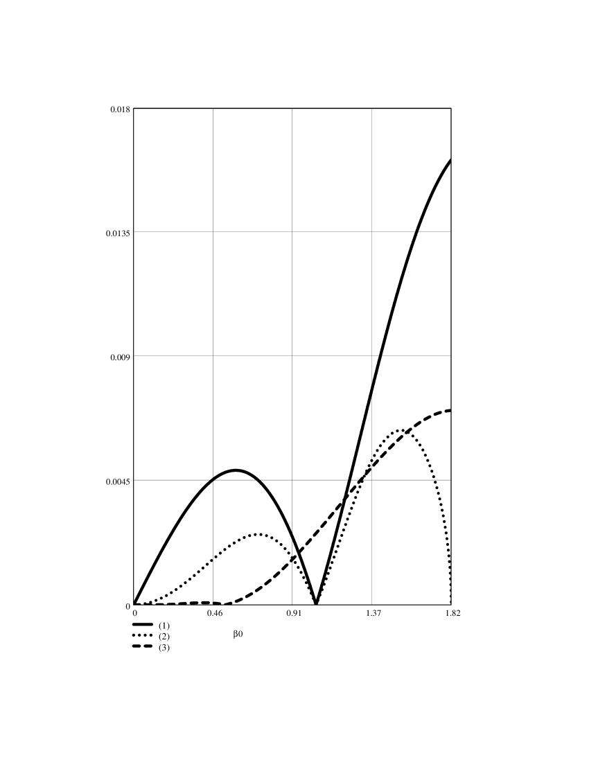
Figure 1: Dependence of increments for two spin waves modes: (1) - $\lambda_{1}^{(1)}(\beta^{(0)},\delta_{1}^{(0)})/\omega_{L}$ (26), (2) - $\lambda_{1}^{{}^{\prime}(2)}(\beta^{(0)},\delta_{1}^{{}^{\prime}(0)})/\omega_{L}$ (31), (3) -$\lambda_{2}^{{}^{\prime}(2)}(\beta^{(0)},\delta_{2}^{{}^{\prime}(0)})/\omega_{L}$ (37), on tipping angle $\beta_{0}$ in interval $0\leq\beta<\theta_{0}=\arccos(-\frac{1}{4})$, $\Omega/\omega_{L}=1/2$ for (2) and (3).

References

• [1] Yu.M. Bunkov, V.V. Dmitriev, Yu.M. Mukharsky et al., Europhysics Lett. 8, 645 (1989).
• [2] Yu.M. Bunkov, V.L. Golo, J. Low Temp. Phys. 137, 625 (2004).
• [3] H. Suhl, J. Phys. Chem. Solids, 1, 209 (1957).
• [4] T. Matsushita, R. Nomura, H.H. Hensley et al., J. Low Temp. Phys. 105, 67 (1996).
• [5] T. Ohmi, M. Tsubota, J. Low Temp. Phys. 83, 177 (1991).
• [6] I. A. Fomin, Zh. Exp. Teor. Fiz. 84, 2109Β (1983) [Sov. Phys. JETP 57, 1227Β (1983)].
• [7] L. D. Landau and E. M. Lifshitz, Course of Theoretical Physics, Vol. 1: Mechanics, 4th ed. (Nauka, Moscow, 1988, Pergamon, Oxford, 1989)
• [8] Yu.M. Bunkov, V.V. Dmitriev, A.V. Markelov et al., Phys. Rev. Lett. 65, 867 (1990).
Refer to caption