Model for the free-volume distributions of equilibrium fluids

Abstract

We introduce and test via molecular simulation a simple model for predicting the manner in which interparticle interactions and thermodynamic conditions impact the single-particle free-volume distributions of equilibrium fluids. The model suggests a scaling relationship for the density-dependent behavior of the hard-sphere system. It also predicts how the second virial coefficients of fluids with short-range attractions affect their free-volume distributions.

I Introduction

Liquid-state theory aims to provide a framework that links the interparticle interactions of a fluid with its local structure, thermodynamic properties, and transport coefficients. One of the central quantities for characterizing the structural order is the static structure factor $S(k)$ (or, equivalently, the pair correlation function $g(r)$).Hanson and McDonald (1986) The structure factor can be readily measured by scattering experiments, computed via molecular simulations, or estimated using integral equation theories. Thermodynamic properties of fluids with pairwise interactions can be calculated directly from $S(k)$ using exact relationships from statistical mechanics. Furthermore, many of the nontrivial dynamical behaviors of liquids can be predicted from a knowledge of $S(k)$ using mode-coupling theory and its recent extensions.Hanson and McDonald (1986); Götze (1999); Reichman and Charbonneau (2005)

However, despite its considerable practical value, $S(k)$ cannot provide a comprehensive description of liquid structure mainly because it only contains information about the spatial correlations between pairs of particles. Higher-order correlation functions, or suitable approximations for them, are required to predict structural quantities that depend on the relative positions of three or more particles. A well known example of such a quantity is the single-particle free volume ${v}_{\mathrm{f}}$, illustrated in Fig. 1 . It is defined as the cage of accessible volume that a given particle center could reach from its present state if its neighboring particles were fixed in their current configuration.Hoover et al. (1972) Restated in simple terms, ${v}_{\mathrm{f}}$ quantifies the “breathing room” that a particle has in its local packing environment. The thermodynamic properties of purely athermal (i.e., hard-core) fluids can be formally related to the statistical geometry of their single-particle free volumes.Hoover et al. (1972); Speedy (1981); Speedy and Reiss (1991); Sastry et al. (1998); Corti and Bowles (1999)

The idea that relaxation processes should also be linked to free volumes has a long history in studies of the liquid state,Rahman (1966); Cohen and Turnbull (1959); Cohen and Grest (1979) and it has motivated the development of numerous “free-volume based” models for predicting transport coefficients.Liu et al. (2002) Unfortunately, a general microscopic framework has yet to emerge, in part due to the computational and experimental difficulties associated with measuring and characterizing free volumes. However, recent advances in computational statistical geometrySastry et al. (1998, 1997) have made it possible to efficiently calculate such properties from particle configurations obtained via either experiments (e.g., confocal microscopy of colloidal suspensionsConrad et al. (2005); Dullens et al. (2006)) or computer simulations.Sastry et al. (1998); Debenedetti and Truskett (1999); Starr et al. (2002); Krekelberg et al. (2006) These methods have catalyzed new efforts to quantitatively examine the basic ideas underlying the free-volume perspective for dynamics and, hence, the prospects for developing a successful microscopic theory.

In this article, we contribute to one aspect of this effort by introducing a simple model for predicting the statistical geometry of single-particle free volumes in equilibrium fluids. We use the aforementioned computational tools of statistical geometry to test the predictions of the model for (i) the hard-sphere (HS) fluid and (ii) a fluid of particles with short-ranged, square-well attractions. The former is the standard structural reference fluid for simple liquids. The latter serves as an elementary model for the behavior of suspensions of attractive colloids and globular proteins, whose structures can be strongly influenced by interparticle attractions. As we show, our model suggests a scaling relationship for the density-dependent behavior of the HS system. It also predicts the manner in which the second virial coefficients of fluids with short-range attractions affect their free-volume distributions.

II General Framework

We consider a three-dimensional (3D) equilibrium fluid comprising $N$ identical spherical particles contained in a macroscopic volume $V$ at temperature $T$. The packing fraction is $\eta=N\pi\sigma^{3}/6V$, and the particles interact via a short-range isotropic pair potential $V_{ij}(r)$ of the generic form

$$V_{ij}(r)=\begin{cases}\infty&r<\sigma,\\ u(r)&\sigma\leq r<\sigma(1+\Delta),\\ 0&r\geq\sigma(1+\Delta),\end{cases}$$ (1)

where $\Delta\leq 1$. If one chooses $u(r)=-\epsilon$, then Eq. (1) describes a square-well interaction. Alternatively, the hard-sphere potential is recovered if $\Delta=0$. We are interested in developing a general strategy for predicting how $V_{ij}(r)$, $\eta$, and $T$ affect the statistical properties of the fluid’s single-particle free volumes. To simplify notation, we implicitly non-dimensionalize all lengths from this point forward by the hard-core diameter $\sigma$ of the particles.

The problem described above cannot be treated exactly, and so we make some simplifying approximations that we later assess by comparing our predictions to results obtained via molecular simulations. Our basic working assumption is that the statistical geometry of the free volumes in the 3D fluid at $T$ and $\eta$ can be predicted based on a knowledge of the exact free-volume distribution $f_{1{\mathrm{D}}}$ of the corresponding one-dimensional (1D) fluid at the same temperature $T$ and the scaled packing fraction $\xi=\eta/\eta_{\mathrm{MRJ}}$. We choose $\eta_{\mathrm{MRJ}}=0.64$ to ensure that the close packing limit of the 1D fluid ($\xi=1$) maps onto the maximally random jammed state of the 3D system.Torquato et al. (2000) Our specific idea is that a particle’s free volume in the 3D fluid at $T$ and $\eta$ can be modeled as a cuboid (see Fig. 1) with length $\alpha{x}_{\mathrm{f}}$, height $\alpha{y}_{\mathrm{f}}$, and width $\alpha{z}_{\mathrm{f}}$, where ${x}_{\mathrm{f}}$, ${y}_{\mathrm{f}}$, and ${z}_{\mathrm{f}}$ are independent random variables drawn from $f_{1{\mathrm{D}}}$ at $T$ and $\xi$.

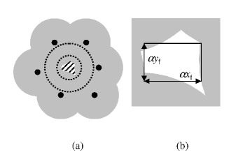
Figure 1: A 2D schematic of the free volume of a tagged particle. Overlapping grey circles represent the exclusion spheres of the neighboring particles. (a) The small dashed circle is the tagged particle surface, and the larger dashed circle is its associated exclusion sphere. The cross-hatched region is the tagged particle’s free volume. (b) An expanded view of the tagged particle’s free volume along with its approximate representation in our model.

The 3D free-volume distribution $f({v}_{\mathrm{f}})$ is thus

$$f({v}_{\mathrm{f}})=\int_{0}^{\infty}\mspace{-15.0mu}dx\!\int_{0}^{\infty}\mspace{-15.0mu}dy\!\int_{0}^{\infty}\mspace{-15.0mu}dz\ \delta({v}_{\mathrm{f}}-\alpha^{3}xyz)\\ \times f_{\mathrm{1D}}(x)f_{\mathrm{1D}}(y)f_{\mathrm{1D}}(z).$$ (2)

The constant $\alpha$ is a scale factor chosen to ensure that our construction accurately reproduces the equilibrium free-volume distributions and thermodynamic properties of the 3D HS fluid (discussed below). Also of interest is the probability density $\phi({s}_{\mathrm{f}})$ associated with finding a 3D free volume with surface area ${s}_{\mathrm{f}}$. Using our model, $\phi({s}_{\mathrm{f}})$ can be expressed as

$$\phi({s}_{\mathrm{f}})=\int_{0}^{\infty}\mspace{-15.0mu}dx\!\int_{0}^{\infty}\mspace{-15.0mu}dy\!\int_{0}^{\infty}\mspace{-15.0mu}dz\ \delta({s}_{\mathrm{f}}-2\alpha^{2}[xy+xz+yz])\\ \times f_{\mathrm{1D}}(x)f_{\mathrm{1D}}(y)f_{\mathrm{1D}}(z).$$ (3)

Eq. (2) and (3) indicate that, in order to predict $f({v}_{\mathrm{f}})$ and $\phi({s}_{\mathrm{f}})$ using our approach, one only needs to derive the state-dependent form of $f_{\mathrm{1D}}$ from knowledge of $V_{ij}(r)$. However, $f_{\mathrm{1D}}$ is given by

$$f_{1{\mathrm{D}}}({x}_{\mathrm{f}})=\int_{0}^{\infty}\mspace{-15.0mu}dy_{L}\!\int_{0}^{\infty}\mspace{-15.0mu}dy_{R}\ \delta({x}_{\mathrm{f}}-y_{L}-y_{R})\\ \times{p_{\mathrm{g}}}(y_{L}){p_{\mathrm{g}}}(y_{R})dy_{L}dy_{R},$$ (4)

where ${p_{\mathrm{g}}}(z)$ is the probability density associated with finding a gap of size $z$ between the surfaces of two neighboring particles in the corresponding 1D fluid. For particles that interact via a pair potential of the form given by Eq. (1), GürseyGürsey (1950) has shown that ${p_{\mathrm{g}}}(z)$ can be written

$${p_{\mathrm{g}}}(z)=\frac{e^{-\beta\Pi[z+1]}e^{-\beta V_{ij}(z+1)}}{\int_{0}^{\infty}e^{-\beta\Pi[s+1]}e^{-\beta V_{ij}(s+1)}ds},$$ (5)

where $\beta=(k_{\mathrm{B}}T)^{-1}$, and $\Pi$ is the 1D pressure. The equation of state of the 1D fluid, i.e., the dependence of $\Pi$ on $\beta$ and $\xi$, can be found implicitly from the following relation:Gürsey (1950)

$$\beta\xi^{-1}=-\left(\frac{\partial\ln\psi}{\partial\Pi}\right)_{T},$$ (6)

where

$$\psi=\int_{0}^{\infty}\mspace{-15.0mu}dx\ e^{-\beta\Pi x}e^{-\beta V_{ij}(x)}.$$ (7)

Having outlined the general strategy of our model, we examine some of its predictions for two specific systems in Section III: (i) the equilibrium HS fluid and (ii) an equilibrium square-well fluid with short-range attractions.

III Testing the model

III.1 Predictions for the HS fluid

Here we apply the model of Section II to predict the statistical geometry of the free volumes in the equilibrium HS fluid, where the pair potential $V_{ij}(r)$ is given by

$$V_{ij}(r)=\begin{cases}\infty&r<1,\\ 0&r\geq 1.\end{cases}$$ (8)

From Eq. (8), (6), and (7), it follows that the equation of state of the 1D HS fluid is given byTonks (1936)

$$\beta\Pi/\xi=1/(1-\xi).$$ (9)

Substituting Eq. (9) and (8) into Eq. (5), yields the corresponding gap-size distribution,

$${p_{\mathrm{g}}}(z)=\frac{\xi}{1-\xi}e^{-z\xi/(1-\xi)}.$$ (10)

Then, from Eq. (4), $f_{\mathrm{1D}}({x}_{\mathrm{f}})$ is simply

$$f_{\mathrm{1D}}({x}_{\mathrm{f}})={x}_{\mathrm{f}}\left(\frac{\xi}{1-\xi}\right)^{2}e^{-{x}_{\mathrm{f}}\xi/(1-\xi)}.$$ (11)

The first moment of this distribution is

$${\langle{x}_{\mathrm{f}}\rangle}\equiv\int_{0}^{\infty}\mspace{-15.0mu}d{x}_{\mathrm{f}}\ {x}_{\mathrm{f}}f_{\mathrm{1D}}({x}_{\mathrm{f}})=\frac{2(1-\xi)}{\xi}.$$ (12)

Defining ${x}_{\mathrm{f}}^{*}\equiv{x}_{\mathrm{f}}/{\langle{x}_{\mathrm{f}}\rangle}$, we have

$$f_{\mathrm{1D}}({x}_{\mathrm{f}})d{x}_{\mathrm{f}}=f_{\mathrm{1D}}^{*}({x}_{\mathrm{f}}^{*})d{x}_{\mathrm{f}}^{*},$$ (13)

where

$$f_{\mathrm{1D}}^{*}({x}_{\mathrm{f}}^{*})=4{x}_{\mathrm{f}}^{*}e^{-2{x}_{\mathrm{f}}^{*}}.$$ (14)

The main implication is that while $f_{\mathrm{1D}}$ is a function of ${x}_{\mathrm{f}}$ and the packing fraction $\xi$ for the 1D HS fluid, $f_{\mathrm{1D}}^{*}({x}_{\mathrm{f}}^{*})$ can be represented by a single curve that is independent of $\xi$. As we show below, this property, when used in combination with Eq. (2) and (3) of our model, leads to scaling predictions for the density-dependent free-volume and free-surface distributions of the 3D HS fluid.

In particular, making use of Eq. (2), (11), and (12), we identify that

$${\langle{v}_{\mathrm{f}}\rangle}\equiv\int_{0}^{\infty}\mspace{-15.0mu}dv\ vf(v)=\alpha^{3}{\langle{x}_{\mathrm{f}}\rangle}^{3}=8\alpha^{3}\left(\frac{1-\xi}{\xi}\right)^{3}.$$ (15)

Similarly, combining Eq. (3), (11), and (12) yields

$${\langle{s}_{\mathrm{f}}\rangle}\equiv\int_{0}^{\infty}\mspace{-15.0mu}ds\ s\phi(s)=6\alpha^{2}{\langle{x}_{\mathrm{f}}\rangle}^{2}=24\alpha^{2}\left(\frac{1-\xi}{\xi}\right)^{2}.$$ (16)

Now, if we normalize the 3D free volume by its first moment, ${v}_{\mathrm{f}}^{*}\equiv{v}_{\mathrm{f}}/{\langle{v}_{\mathrm{f}}\rangle}$, then we have

$$f({v}_{\mathrm{f}})d{v}_{\mathrm{f}}=f^{*}({v}_{\mathrm{f}}^{*})d{v}_{\mathrm{f}}^{*},$$ (17)

where

$$f^{*}({v}_{\mathrm{f}}^{*})=\int_{0}^{\infty}\mspace{-15.0mu}dx\!\int_{0}^{\infty}\mspace{-15.0mu}dy\!\int_{0}^{\infty}\mspace{-15.0mu}dz\ \delta({v}_{\mathrm{f}}^{*}-xyz)\\ \times f_{\mathrm{1D}}^{*}(x)f_{\mathrm{1D}}^{*}(y)f_{\mathrm{1D}}^{*}(z).$$ (18)

Similarly, if we introduce the reduced free surface ${s}_{\mathrm{f}}^{*}\equiv{s}_{\mathrm{f}}/{\langle{s}_{\mathrm{f}}\rangle}$, then it follows that

$$\phi({s}_{\mathrm{f}})d{s}_{\mathrm{f}}=\phi^{*}({s}_{\mathrm{f}}^{*})d{s}_{\mathrm{f}}^{*},$$ (19)

where

$$\phi^{*}({s}_{\mathrm{f}}^{*})=\int_{0}^{\infty}\mspace{-15.0mu}dx\!\int_{0}^{\infty}\mspace{-15.0mu}dy\!\int_{0}^{\infty}\mspace{-15.0mu}dz\ \delta({s}_{\mathrm{f}}^{*}-[xy+xz+yz]/3)\\ \times f_{\mathrm{1D}}^{*}(x)f_{\mathrm{1D}}^{*}(y)f_{\mathrm{1D}}^{*}(z).$$ (20)

Eq. (18) and (20), when viewed together with Eq. (14), show that our model predicts that the scaled free-volume and free-surface distributions, $f^{*}({v}_{\mathrm{f}}^{*})$ and $\phi^{*}({s}_{\mathrm{f}}^{*})$, are independent of packing fraction for the 3D HS fluid. We will return to this point later, when we test the predictions of the model via molecular simulations.

To use the model to predict the shapes of the free volumes in the 3D HS fluid, we analyze the behavior of the dimensionless sphericity parameter $\lambda_{\mathrm{f}}$, defined asRuocco and Sampoli (1991, 1992)

$$\lambda_{\mathrm{f}}={s}_{\mathrm{f}}(6\pi^{1/2}{v}_{\mathrm{f}})^{-2/3}.$$ (21)

The sphericity parameter takes on its minimum possible value ($\lambda_{\mathrm{f}}=1$) for a spherical free volume, while it is larger in magnitude for less symmetric free volumes. Our model predicts that the average value of the sphericity parameter (quantifying the average shape of the free volumes), given by

$$\langle\lambda_{\mathrm{f}}\rangle=\int_{0}^{\infty}\mspace{-15.0mu}dx\!\int_{0}^{\infty}\mspace{-15.0mu}dy\!\int_{0}^{\infty}\mspace{-15.0mu}dz\ \frac{2(xy+xz+yz)}{(6\pi^{1/2}xyz)^{2/3}}\\ \times f_{\mathrm{1D}}(x)f_{\mathrm{1D}}(y)f_{\mathrm{1D}}(z)\simeq 1.57,$$ (22)

is independent of packing fraction for the 3D HS fluid.

Finally, the equation of state of the 3D HS fluid can be formally related to the statistical geometry of its free volumes:Hoover et al. (1972); Speedy (1981); Sastry et al. (1998)

$$\frac{\beta P}{\rho}=1+\frac{1}{6}\left<\frac{{s}_{\mathrm{f}}}{{v}_{\mathrm{f}}}\right>.$$ (23)

Here, $P$ is the pressure of the 3D fluid, and $\rho=N/V$ is its number density. In our model, it is easily shown that

$$\left<\frac{{s}_{\mathrm{f}}}{{v}_{\mathrm{f}}}\right>=\int_{0}^{\infty}\mspace{-15.0mu}dx\!\int_{0}^{\infty}\mspace{-15.0mu}dy\!\int_{0}^{\infty}\mspace{-15.0mu}dz\ \frac{2(xy+xz+yz)}{\alpha xyz}\\ \times f_{\mathrm{1D}}(x)f_{\mathrm{1D}}(y)f_{\mathrm{1D}}(z)=\frac{6\alpha^{-1}\xi}{1-\xi},$$ (24)

and therefore we have

$$\frac{\beta P}{\rho}=\frac{1-(1-\alpha^{-1})\xi}{1-\xi}.$$ (25)

III.2 Simulations of the HS Fluid

To test the predictions of our free-volume model for the 3D equilibrium HS fluid, we have performed a series of molecular dynamics simulations using a standard event-driven algorithm.Rapaport (2004) All runs were carried out in the microcanonical ensemble using $N=1000$ particles and a periodically-replicated cubic simulation cell. Snapshots of the system’s equilibrium configurations were collected and used to calculate the geometric properties of single-particle free volumes via the exact algorithm presented by Sastry et al..Sastry et al. (1998, 1997)

Numerical predictions using the free-volume model introduced here require specifying the value of the geometric scale factor $\alpha$ shown in Fig. 1. As discussed in Section II, the goal is to choose $\alpha$ in a way that allows the model to provide a reasonable overall description of the statistical geometry, and hence the thermodynamic properties, of the HS fluid. Throughout this work we set $\alpha=0.29$, which we obtained from a least-squares fit of Eq. (15) to the HS simulation data for ${\langle{v}_{\mathrm{f}}\rangle}$ versus $\eta$ over the range $0.375\leq\eta\leq 0.525$. The quality of this fit is illustrated in the inset of Fig. 2a.

We also compare in Fig. 2a the free-volume distributions $f({v}_{\mathrm{f}})$ obtained from simulations with those predicted via Eq. (2). We observe that the model describes the data relatively well, with the predictions becoming semi-quantitative for the higher packing fractions investigated. This trend with packing fraction is expected since the simulated free volumes become more compact at higher densities, and, as a result, they more closely resemble the simple cuboid shapes that we have assumed in our model.

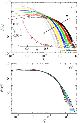
Figure 2: (a) Free-volume distributions of the 3D HS fluid for packing fractions $\eta=0.375,\ 0.4,\ 0.425,\ 0.45,\ 0.475,\ 0.5,$ and $0.525$. Symbols are simulation data and solid curves are the predictions of Eq. (2). The arrow indicates increasing packing fraction $\eta$. Inset: Average free volume ${\langle{v}_{\mathrm{f}}\rangle}$ versus packing fraction $\eta$. Circles are simulation data and the solid line is the prediction of Eq. (15). (b) Probability density associated with observing particles with scaled free volume ${v}_{\mathrm{f}}^{*}={v}_{\mathrm{f}}/{\langle{v}_{\mathrm{f}}\rangle}$. Symbols are simulation data from panel (a) and the solid line is the prediction of Eq. (18).

The same free-volume distributions shown in Fig. 2a are also shown in Fig. 2b, only now scaled in the manner suggested by Eq. (18). This rescaling yields the probability density associated with observing a particle with a particular value of ${v}_{\mathrm{f}}^{*}={v}_{\mathrm{f}}/{\langle{v}_{\mathrm{f}}\rangle}$. Interestingly, we observe that, to a very good approximation, the scaled distributions obtained via simulation for all packing fractions investigated collapse onto a single curve predicted by the model.

As can be seen by Eq. (20), the model predicts that the distributions of free surfaces for the HS fluid should also collapse onto a single curve when scaled in an analogous way. We compare in Fig. 3a the scaled free-surface distributions $\phi^{*}({s}_{\mathrm{f}}^{*})$ obtained via simulation to the predictions of Eq. (20). Again, the collapse of the simulation data is striking, and it is described reasonably well by the free-volume model. The inset of Fig. 3a compares the average free-surface area per particle ${\langle{s}_{\mathrm{f}}\rangle}$ obtained from simulations to the prediction of Eq. (16). As with the predictions for $f({v}_{\mathrm{f}})$, the model provides a more accurate description of ${\langle{s}_{\mathrm{f}}\rangle}$ at higher packing fractions where the free volumes are expected to be more compact. At low packing fractions, particles will on average have more nearest neighbors which define their free-volume then at high packing . Therefore, we expect our cuboid approximation to break down at low packing fractions.

To quantify the compactness of the HS free volumes, we compare in Fig. 3b the average sphericity of the free volumes $\left<\lambda_{\mathrm{f}}\right>$ calculated from the simulations to that predicted by Eq. (22). We find that while the cuboid representation of free volumes in our model underestimates $\left<\lambda_{\mathrm{f}}\right>$, it qualitatively captures the fact that, on average, the shapes of the free volumes in the HS fluid are fairly insensitive to changes in packing fraction.

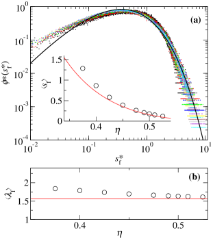
Figure 3: (a) Proabability density associated with observing particles with scaled free surface area ${s}_{\mathrm{f}}^{*}={s}_{\mathrm{f}}/{\langle{s}_{\mathrm{f}}\rangle}$ in the 3D HS fluid for packing fractions $\eta=0.375,\ 0.4,\ 0.425,\ 0.45,\ 0.475,\ 0.49,\ 0.5,\ 0.51$, and 0.525. Symbols are simulation data and solid curves are the predictions of Eq. (20). Inset: Average free surface area ${\langle{s}_{\mathrm{f}}\rangle}$ versus packing fraction $\eta$. Circles are simulation data and the solid line is the prediction of Eq. (16). (b) Average sphericity $\left<\lambda_{\mathrm{f}}\right>$ of free volumes in the HS fluid versus packing fraction $\eta$. Circles are simulation data, and the solid line is the prediction of Eq. (22).

Finally, we test the ability of our free-volume model to predict the equation of state of the HS system. In particular, we compare Eq. (25) to the well-known Carnahan-StarlingCarnahan and Starling (1969) equation, which provides an accurate description of the HS pressure for packing fractions in the equilibrium fluid range $0<\eta<0.494$.

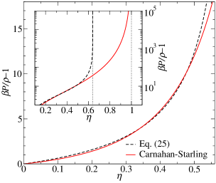
Figure 4: Equation of state for the HS fluid as calculated from both Eq. (25) and the Carnahan-StarlingCarnahan and Starling (1969) relationship. Inset: Expanded version illustrating that Eq. (25) diverges at $\eta_{\mathrm{MRJ}}=0.64$, while the Carnahan-Starling relationship diverges at the unphysically high packing fraction of $\eta=1$.

As can be seen in Fig. 4, Eq. (25) shows good agreement with the Carnahan-Starling equation for the equilibrium HS fluid. Moreover, while the Carnahan-Starling equation diverges at the unphysically high packing fraction of $\eta=1$, Eq. (25) predicts that the HS fluid becomes incompressible at the packing fraction of the maximally random jammed state ($\eta_{\mathrm{MRJ}}=0.64$).Torquato et al. (2000)

III.3 Predictions for the Square-Well Fluid

To demonstrate that the ideas outlined in Section II can be readily extended to other fluid systems, we now use our approach to predict the free-volume distributions of a square-well fluid with short-range attractions, a basic model system for suspensions of attractive colloids and globular proteins. Fluids with short-ranged attraction are of particular interest here because they exhibit free-volume distributions with shapes that differ from that of the equilbrium HS fluid at the same packing fraction.Krekelberg et al. (2006) Specifically, interparticle clustering induced by the short-range attractions increases the populations of both large and small free volumes at the expense of mid-sized free volumes. These structural changes play an important role in the anomalous dynamical properties exhibited by these fluids,Krekelberg et al. (2006) and the ability to predict such changes constitutes a sensitive test of our free-volume model.

The square-well pair potential is given by

$$V_{ij}(r)=\begin{cases}\infty&r<1,\\ -\epsilon&1\leq r<1+\Delta,\\ 0&r\geq 1+\Delta.\end{cases}$$ (26)

Using Eq. (26), (6), and (7), one can show that the equation of state of the 1D square-well fluid can be expressed as

$$\xi^{-1}=1+\frac{1}{\beta\Pi}+\frac{\Delta e^{-\beta\Pi\Delta}(1-e^{-\beta\epsilon})}{1-e^{-\beta\Pi\Delta}(1-e^{-\beta\epsilon})}.$$ (27)

Furthermore, by substituting Eq. (5), (26), and (27) into Eq. (4), one finds that the corresponding 1D free-volume distribution is given by

$$\frac{f_{\mathrm{1D}}({x}_{\mathrm{f}})}{\Theta({x}_{\mathrm{f}})}=\begin{cases}{x}_{\mathrm{f}}&{x}_{\mathrm{f}}<\Delta,\\ 2e^{-\beta\epsilon}({x}_{\mathrm{f}}-\Delta)-{x}_{\mathrm{f}}+2\Delta&{x}_{\mathrm{f}}\in[\Delta,2\Delta),\\ {x}_{\mathrm{f}}e^{-2\beta\epsilon}+2\Delta e^{-\beta\epsilon}(1-e^{-\beta\epsilon})&{x}_{\mathrm{f}}\geq 2\Delta,\end{cases}$$ (28)

where

$$\Theta({x}_{\mathrm{f}})=e^{-\beta\Pi{x}_{\mathrm{f}}}\left[\frac{\beta\Pi}{1-e^{-\beta\Pi\Delta}(1-e^{-\beta\epsilon})}\right]^{2}.$$ (29)

By substituting Eq. (28) into Eq. (2), one can readily calculate the free-volume distribution for the 3D square-well fluid numerically.

III.4 Simulations of the Square-Well Fluid

To test the theoretical predictions of our model for the 3D square-well fluid, we have performed a series of event-driven molecular dynamics simulationsRapaport (2004) using $N=1000$ particles. As with the HS simulations described earlier, a cubic simulation cell was employed with periodic boundary conditions. Equilibrium configurations were stored during these runs and later used to calculateSastry et al. (1998, 1997) the geometric properties of the single-particle free volumes. For all simulations, the range of the square-well attraction was set to $\Delta=0.03$. We studied the fluid at packing fraction $\eta=0.5$ and $0.58$. For the $\eta=0.58$ case, a flat distribution of particles sizes with mean $\sigma$ and half width $\delta=\sigma/10$ was used to prevent crystallization. We examined the behavior of the fluid for various values of the strength of the interparticle attraction $\epsilon$, which is often quantified using the reduced second virial coefficient $B_{2}^{*}=B_{2}/B_{2}^{\mathrm{HS}}$. Here, $B_{2}=(1/2)\int d{\bf r}[1-\exp(-\beta V_{ij}(|{\bf r}|))]$ is the second virial coefficient of the fluid of interest, and $B_{2}^{\mathrm{HS}}=2\pi/3$ is that of the hard-sphere fluid. For the 3D square-well fluid, $B_{2}^{*}$ is given by

$$\begin{split}B_{2}^{*}&=3\int_{0}^{\infty}r^{2}[1-e^{-\beta V_{ij}(r)}]dr\\ &=1+(1-e^{\beta\epsilon})[(1+\Delta)^{3}-1].\end{split}$$ (30)

The simulated results for the free-volume distributions are displayed in Fig. 5a and 5b for $\eta=0.5$ and $0.58$, respectively. As has been observed for other model fluids with short-range attractions,Krekelberg et al. (2006) decreasing $B_{2}^{*}$ (increasing attractions) increases the populations of both large and small free volumes at the expense of the mid-sized free volumes. These trends are captured by the predictions of the free-volume model (Fig. 5b and 5d) using Eq. (2), (28), and (29). It is evident that the model does not match the simulation results as well at $\eta=0.58$ as at $\eta=0.5$. This is most likely due to the 1D equation of state used in the model being less accurate at high packing fractions. Although the free-volume model presented here does not reproduce the square-well distributions with quanitative accuracy, it clearly captures the important physical trends. Moreover, its predictions show surprisingly good agreement with the simulation data, given that there are no free parameters in the theory that are fit to data for the square-well fluid.

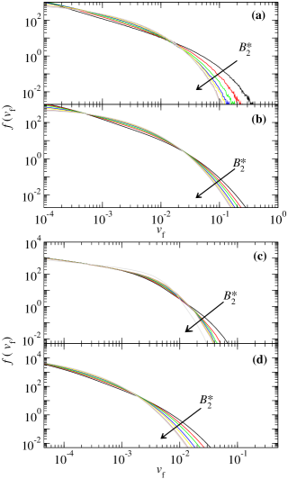
Figure 5: Free-volume distributions for the square-well fluid at range of attraction $\Delta=0.03$, and reduced second virial coefficients $B_{2}^{*}=-0.04,\ 0.41,\ 0.60,\ 0.78,\ 0.84,\ 0.91,$ and $0.94$. (a) Simulations at packing fraction $\eta=0.5$ and (b) the free-volume model at described in the text at $\eta=0.5$. (c) Simulations at packing fraction $\eta=0.58$ and (d) free-volume model at $\eta=0.58$. Arrows indicate increasing $B_{2}^{*}$.

IV Conclusions

In summary, we have introduced a simple model for predicting the free-volume distributions of equilibrium fluids, and we have tested this model using molecular simulations. The model suggests a new scaling for the density-dependencies of the free-volume and free-surface distributions of the HS fluid, and these scalings show very good agreement with simulation results. The free-volume model also predicts a reasonably accurate hard-sphere equation of state in which the pressure diverges at a packing fraction of $\eta=0.64$. Finally, the model predicts semi-quantitatively the manner in which the attractive strength affects the free-volume distributions of a square-well fluid with short-range attractions. These considerations suggest that the free-volume model proposed here can perhaps be used fruitfully within the free-volume based theories for dynamics of fluids to understand how their transport coefficients derive from their microscopic interactions and thermodynamic conditions.

Acknowledgments. WPK acknowledges financial support of the National Science Foundation for a Graduate Research Fellowship. TMT acknowledges financial support of the National Science Foundation (CTS 0448721) and the David and Lucile Packard Foundation, and VG acknowledges financial support of the Robert A. Welch Foundation and the Alfred P. Sloan Foundation. Simulations were performed at the Texas Advanced Computing Center (TACC).

References

- Hanson and McDonald (1986) J. P. Hanson and I. R. McDonald, Theory of Simple Liquids (Academic, London, 1986), 2nd ed.
- Götze (1999) W. Götze, J. Phys. Condens. Matter 11, A1 (1999).
- Reichman and Charbonneau (2005) D. R. Reichman and P. Charbonneau, J. Stat. Mech. P05013 (2005).
- Hoover et al. (1972) W. G. Hoover, W. T. Ashurst, and R. Grover, J. Chem. Phys. 57, 1259 (1972).
- Speedy (1981) R. J. Speedy, J. Chem. Soc., Faraday Trans. 2 77, 329 (1981).
- Speedy and Reiss (1991) R. J. Speedy and H. Reiss, Mol. Phys. 72, 1015 (1991).
- Sastry et al. (1998) S. Sastry, T. M. Truskett, P. G. Debenedetti, and S. Torquato, Mol. Phys. 95, 289 (1998).
- Corti and Bowles (1999) D. S. Corti and R. K. Bowles, Mol. Phys. 96, 1623 (1999).
- Rahman (1966) A. Rahman, J. Chem. Phys. 45, 2585 (1966).
- Cohen and Turnbull (1959) M. H. Cohen and D. Turnbull, J. Chem. Phys. 31, 1164 (1959).
- Cohen and Grest (1979) M. H. Cohen and G. S. Grest, Phys. Rev. B 20, 1077 (1979).
- Liu et al. (2002) H. Liu, C. M. Silva, and E. A. Macedo, Fluid Phase Equilib. 202, 89 (2002).
- Sastry et al. (1997) S. Sastry, D. S. Corti, P. G. Debenedetti, and F. H. Stillinger, Phys. Rev. E 56, 5524 (1997).
- Conrad et al. (2005) J. C. Conrad, F. W. Starr, and D. A. Weitz, J. Phys. Chem. B 109, 21235 (2005).
- Dullens et al. (2006) R. P. A. Dullens, D. G. A. L. Aarts, and W. K. Kegel, Proc. Natl. Acad. Sci. USA 103, 529 (2006).
- Debenedetti and Truskett (1999) P. G. Debenedetti and T. M. Truskett, Fluid Phase Equilib. 158, 549 (1999).
- Starr et al. (2002) F. W. Starr, S. Sastry, J. F. Douglas, and S. C. Glotzer, Phys. Rev. Lett. 89, 125501 (2002).
- Krekelberg et al. (2006) W. P. Krekelberg, V. Ganesan, and T. M. Truskett, J. Phys. Chem. B 110, 5166 (2006).
- Torquato et al. (2000) S. Torquato, T. M. Truskett, and P. G. Debenedetti, Phys. Rev. Lett. 84, 2064 (2000).
- Gürsey (1950) F. Gürsey, Proc. Cambridge Philos. Soc 46, 182 (1950).
- Tonks (1936) L. Tonks, Phys. Rev. 50, 955 (1936).
- Ruocco and Sampoli (1991) G. Ruocco and M. Sampoli, J. Mol. Struct. 250, 171 (1991).
- Ruocco and Sampoli (1992) G. Ruocco and M. Sampoli, Chem. Phys. Lett. 188, 332 (1992).
- Rapaport (2004) D. C. Rapaport, The Art of Molecular Dynamic Simulation (Cambridge University Press, Cambridge, 2004), 2nd ed.
- Carnahan and Starling (1969) N. F. Carnahan and K. E. Starling, J. Chem. Phys. 51, 635 (1969).