SYMMETRIC $(q,\alpha)$-STABLE DISTRIBUTIONS.
PART II: SECOND REPRESENTATION

Abstract

This paper is a continuation of papers [1, 2]. In Part I [2] a description (representation) of $(q,\alpha)$-stable distributions based on a $F_{q}$-transform was given. Here, in Part II, we present another description of these distributions. This approach generalizes results of [1] (which corresponds to $\alpha=2,\,Q\in[1,3)$) to the whole range of stability and nonextensivity parameters $\alpha\in(0,2]$ and $Q\in[1,3),$ respectively. The present case $\alpha=2$ recovers the $q$-Gaussian distributions. Similar to what is discussed in [1], a triplet $(q^{\ast},q,q_{\ast})$ arises for which the mapping $F_{q^{\ast}}:\,\mathcal{G}_{q}\rightarrow\mathcal{G}_{q_{\ast}}$ holds. Moreover, by unifying the two preceding descriptions, further possible extensions are discussed and some conjectures are formulated.

1 Introduction

In the paper [1], and in Part I [2] of the current paper, we discussed a $q$-generalization of the classic central limit theorem (see also [3, 4]) applicable to nonextensive statistical mechanics, (see [5, 6, 7] and references therein), and $q$-generalization of $\alpha$-stable Lévy distributions (see, e.g., [8, 9, 10, 11]). The obtained generalizations concern random variables with a special long-range correlations arising in nonextensive statistical mechanics. In [1] we introduced $q$-Fourier transform and the function $z(s)={(1+s)}/{(3-s)}$ to describe attractors of scaling limits of sums of $q$-independent random variables with a finite $(2q-1)$-variance . This description was essentially based on the mapping

$$F_{q}:\mathcal{G}_{q}\rightarrow\mathcal{G}_{z(q)},$$ (1)

where $\mathcal{G}_{q}$ is the set of $q$-Gaussians.

In Part I we introduced the set $\mathcal{L}_{q}(\alpha)$ of $(q,\alpha)$-stable distributions with associated densities having asymptotic behavior $f\sim C|x|^{-\phi(q,\alpha)},\,|x|\rightarrow\infty,$ where $\phi(q,\alpha)=\frac{\alpha+1}{1+\alpha(q-1)},$ $0<\alpha<2,\,1\leq q<2$, and $C>0$ is a constant. The corresponding random variables have infinite $Q$-variance ($Q=2q-1$) for all $0<\alpha<2$ and $1\leq Q<3.$ Their representation was obtained through the map

$$F_{q}:\mathcal{G}_{q^{L}}[2]\rightarrow\mathcal{G}_{q}[\alpha],$$ (2)

where $\mathcal{G}_{q}[\alpha]=\{be_{q}^{-\beta|\xi|^{\alpha}},\,b>0,\,\beta>0\}$ and

$$q^{L}=\frac{3+Q\alpha}{\alpha+1},\,Q=2q-1.$$

Recall that the parameters $Q$ and $\alpha$ range in the set $\mathcal{Q}=\{1\leq Q<3,\,\,0<\alpha\leq 2\},$ and in the framework of this description, the value $\alpha=2$ was peculiar. For the convenience of the reader we also reproduce the following lemma proved in Part I, which plays a key role in the current description as well.

Lemma 1.1

Let $f(x),\,x\in R,$ be a symmetric probability density function of a given random variable. Further, let either

• the $(2q-1)$-variance $\sigma_{2q-1}^{2}<\infty,$ (associated with $\alpha=2$), or

• $f(x)\in H_{q,\alpha}$, where $(2q-1,\alpha)\in\mathcal{Q}_{2}.$

Then for the $q$-Fourier transform of $f(x)$ the following asymptotic relation holds true:

$$F_{q}[f](\xi)=1-\mu_{q,\alpha}|\xi|^{\alpha}+o(|\xi|^{\alpha}),\xi\rightarrow 0,$$ (3)

where

$$\mu_{q,\alpha}=\left\{\begin{array}[]{ll}\vspace{1cm}\frac{q}{2}\sigma_{2q-1}^{2}\nu_{2q-1},&\mbox{if $\alpha=2$;}\\ \ \frac{2^{2-\alpha}(1+\alpha(q-1))}{2-q}\int_{0}^{\infty}\frac{-\,\Psi_{q}(y)}{y^{\alpha+1}}dy,&\mbox{if $0<\alpha<2$,}\end{array}\right.$$ (4)

where $\nu_{2q-1}(f)=\int_{-\infty}^{\infty}[f(x)]^{2q-1}\,dx$, and $\Psi_{q}(y)=\cos_{q}(2x)-1.$

In Part II we represent second description of $(q,\alpha)$-stable distributions. In the frame of the new description the value $\alpha=2$ is no longer peculiar, but in this case we need to separate the value $q=1.$ More precisely, we expand the result of the paper [1] to the region

$$\mathcal{Q}=\{(Q,\alpha):1\leq Q<3,0<\alpha\leq 2\},$$

generalizing the mapping (1) in the form

$$F_{\zeta_{\alpha}(q)}:\mathcal{G}_{q}[\alpha]\rightarrow\mathcal{G}_{z_{\alpha}(q)}[\alpha],\,1\leq q<2,\,0<\alpha\leq 2,$$ (5)

where

$$\zeta_{\alpha}(s)=\frac{\alpha+2(q-1)}{\alpha}\,\,\mbox{and}\,\,z_{\alpha}(s)=\frac{\alpha q-(q-1)}{\alpha-(q-1).}$$

Note that if $\alpha=2$, then $\zeta_{2}(q)=q,$ $z_{2}(q)=(1+q)/(3-q),$ and $\mathcal{G}_{q}[2]=\mathcal{G}_{q},$ recovering the mapping (1).

2 $(q,\alpha)$-stable distributions. Second description

Let $1<q<2$, or equivalently, $1<Q<3,\,\,Q=2q-1$. It follows from the definition of the $q$-exponential that any density function $g\in\mathcal{G}_{q}[\alpha]$ has the asymptotic behavior $g\sim b\,|x|^{-\alpha\over{q-1}},\,b>0,$ for large $|x|$. The set of all functions with this asymptotic we denote by $\mathcal{B}_{q}[\alpha]$. It is readily seen that $\mathcal{G}_{q}[\alpha]\subset\mathcal{B}_{q}[\alpha]$. At the same time, for any density $f\in\mathcal{B}_{q}[\alpha]$, there exists a unique density $g\in\mathcal{G}_{q}[\alpha]$, such that $f\sim g,\,\,|x|\rightarrow\infty.$ In this sense the two sets $\mathcal{G}_{q}[\alpha]$ and $\mathcal{B}_{q}[\alpha]$ are asymptotically equivalent (or asymptotically equal). Having this in mind we write (preferably) $\mathcal{G}_{q}[\alpha]$ instead of $\mathcal{B}_{q}[\alpha].$

Lemma 2.1

Let $0<\alpha\leq 2$ be fixed. For arbitrary $q_{1}$ there exists $q_{2}$ and a one-to-one mapping $\mathcal{M}_{q_{1},q_{2}}$ such that

$$\mathcal{M}_{q_{1},q_{2}}:\mathcal{G}_{q_{1}}[\alpha]\rightarrow\mathcal{G}_{q_{2}}[2].$$

Obviously, if $\alpha=2$, then $q_{1}=q_{2}$ and $\mathcal{M}_{q_{1},q_{2}}$ is the identity operator. First we find the relationship between the three indices $q$, $q^{\ast}$ and $q_{\ast}$ for which the mapping

$$F_{q^{\ast}}:\mathcal{G}_{q}[\alpha]\stackrel{{\scriptstyle(a)}}{{\rightarrow}}\mathcal{G}_{q_{\ast}}[\alpha],$$ (6)

where $\stackrel{{\scriptstyle(a)}}{{\rightarrow}}$ means that the mapping is in the sense of the asymptotic equivalence explained above, holds with $\alpha\in(0,2]$. The exact meaning of (6) is

$$\mathcal{M}^{-1}_{q_{\ast},z(q_{\ast})}F_{q^{\ast}}\mathcal{M}_{q,q^{\ast}}:\mathcal{G}_{q}[\alpha]\rightarrow\mathcal{G}_{q_{\ast}}[\alpha].$$

In the case $\alpha=2$, as we mentioned above, $\mathcal{M}_{q_{1},q_{2}}=I,$ and the relationships $q^{\ast}=q$ and $q_{\ast}=\frac{1+q}{3-q}$ were found in [1], giving (1).

Lemma 2.2

Assume $0<\alpha\leq 2$ and let the numbers $q^{\ast},\,\,q_{\ast}$ and $q$ be connected with the relationships

$$q^{\ast}=\frac{\alpha-2(q-1)}{\alpha}\,\,\mbox{and}\,\,q_{\ast}=\frac{\alpha q+(q-1)}{\alpha+(q-q).}$$ (7)

Then the mapping (6) holds true.

Proof. Let $f\in\mathcal{G}_{q}[\alpha]$, which means that asymptotically $f(x)\sim b\,|x|^{-\alpha/(q-1)},\\ x\rightarrow\infty$ with some $b>0$. We find the $q^{\ast}$-Gaussian with the same asymptotics at infinity. For a $q^{\ast}$-Gaussian $G_{q^{\ast}}(\beta;x),\,\,(\beta>0),$ to be asymptotically equivalent to $f,$ it is necessary

$$G_{q^{\ast}}(\beta;x)\sim\frac{C}{|x|^{2\over{q^{\ast}-1}}}\sim\frac{b}{|x|^{\alpha\over{q-1}}},\,\,|x|\rightarrow\infty,$$

where $C>0$ and $b>0$ some constants. Hence

$$q^{\ast}=\frac{\alpha+2(q-1)}{\alpha}=1+\frac{2(q-1)}{\alpha}.$$

Further, it follows from Corollary 2.10 of [1], that

$$F_{q^{\ast}}:\,\,\mathcal{G}_{q^{\ast}}[2]\rightarrow\mathcal{G}_{q_{1}}[2],$$

where

$$q_{1}=\frac{1+q^{\ast}}{3-q^{\ast}}=\frac{\alpha+(q-1)}{\alpha-(q-1)}.$$

Further, taking into account the asymptotic equality

$$G_{q_{1}}(\beta_{1};x)\sim\frac{C}{|x|^{2\over{q_{1}-1}}}\sim\frac{C}{|x|^{{\alpha}\over{q_{\ast}-1}}},\,\,|x|\rightarrow\infty,$$

we obtain

$$q_{\ast}=\frac{\alpha q-(q-1)}{\alpha-(q-1)}=1+\frac{\alpha(q-1)}{\alpha-(q-1)}.$$

Thus, the mapping (6) holds with $q^{\ast}$ and $q_{\ast}$ in Equation (7).  

Let us now introduce two functions that are important for our further analysis:

$$z_{\alpha}(s)=\frac{\alpha s-(s-1)}{\alpha-(s-1)}=1+\frac{\alpha(s-1)}{\alpha-(s-1)},\,\,0<\alpha\leq 2,\,\,s<\alpha+1\,,$$ (8)

and

$$\zeta_{\alpha}(s)=\frac{\alpha+2(s-1)}{\alpha}=1+\frac{2(s-1)}{\alpha},\,\,0<\alpha\leq 2\,.$$ (9)

It can be easily verified that $\zeta_{\alpha}(s)=s$ if $\alpha=2.$

The inverse, $z_{\alpha}^{-1}(t),\,t\in(1-\alpha,\infty)$, of the the first function reads

$$z_{\alpha}^{-1}(t)=\frac{\alpha t+(t-1)}{\alpha+(t-1)}=1+\frac{\alpha(t-1)}{\alpha+(t-1)}\,.$$ (10)

The function $z(s)$ possess the properties: $z_{\alpha}(\frac{1}{z_{\alpha}(s)})={1\over s}$ and $z_{\alpha}({1\over s})={1\over z_{\alpha}^{-1}(s)}\,.$ If we denote $q_{\alpha,1}=z_{\alpha}(q)$ and $q_{\alpha,-1}=z_{\alpha}^{-1}(q),$ then

$$z_{\alpha}({1\over q_{\alpha,1}})={1\over q}\,\,\,\,\,\mbox{and}\,\,\,\,\,z_{\alpha}({1\over q})={1\over q_{\alpha,-1}}\,.$$ (11)

Corollary 2.3

Let $0<\alpha\leq 2$ and $1\leq q<\min\{2,1+\alpha\}.$ Then the following mapping

$$F_{\zeta_{\alpha}(q)}:\mathcal{G}_{q}(\alpha)\stackrel{{\scriptstyle(a)}}{{\rightarrow}}\mathcal{G}_{z_{\alpha}(q)}(\alpha),$$

holds.

Corollary 2.4

There exists the following inverse $q$-Fourier transform

$$F^{-1}_{\zeta_{\alpha}(q)}:\mathcal{G}_{z_{\alpha}(q)}(\alpha)\stackrel{{\scriptstyle(a)}}{{\rightarrow}}\mathcal{G}_{q}(\alpha),\,\,\,q<\min\{2,1+\alpha\},$$

Using the above mentioned properties of the function $z_{\alpha}(s)$ we can derive a number of useful formulas for the $q$-Fourier transforms. For instance, if $q<1$, then we have the mappings

$$F_{\zeta_{\alpha}(\frac{1}{q_{\alpha,1}})}:\,\,\,\mathcal{G}_{\frac{1}{q_{\alpha,1}}}(\alpha)\stackrel{{\scriptstyle(a)}}{{\rightarrow}}\mathcal{G}_{\frac{1}{q}}(\alpha),$$

$$F_{\zeta_{\alpha}(\frac{1}{q})}:\,\,\,\mathcal{G}_{\frac{1}{q}}(\alpha)\stackrel{{\scriptstyle(a)}}{{\rightarrow}}\mathcal{G}_{\frac{1}{q_{\alpha,-1}}}(\alpha).$$

The analogous formulas hold for the inverse $q$-Fourier transforms as well.

Introduce the sequence $q_{\alpha,n}=z_{\alpha,n}(q)=z(z_{\alpha,n-1}(q)),n=1,2,...,$ with a given $q=z_{0}(q),\,q<1+\alpha.$ We can extend the sequence $q_{\alpha,n}$ for negative integers $n=-1,-2,...$ as well putting $q_{\alpha,-n}=z_{\alpha,-n}(q)=z_{\alpha}^{-1}(z_{\alpha,1-n}(q)),n=1,2,...\,.$ It is not hard to verify that

$$q_{\alpha,n}=1+\frac{\alpha(q-1)}{\alpha-n(q-1)}=\frac{\alpha q-n(q-1)}{\alpha-n(q-1)},\,\,-\infty<n\leq[\frac{\alpha}{q-1}].$$ (12)

The restriction $n\leq[\alpha/(q-1)]$ on the right hand side of (12) comes from intension to have $q_{\alpha,n}>1,$ since $q$-Fourier transform is defined for $q\geq 1.$ (See Fig. 1 for $q_{\alpha,n}$ with some typical values of $\alpha$ and $n$).

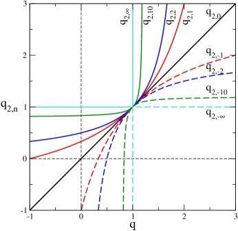
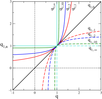
Figure 1: The $q$-dependences of $q_{2,n}$ (top) and $q_{1,n}$ (bottom) as given by Eq. (12). We notice the tendency of all the $|n|\to\infty$ curves to collapse onto the $q_{\alpha,n}=1$ horizontal straight line if $q\neq 1$, and onto the $q=1$ vertical straight line if $q=1$. This tendency is gradually intensified, $\forall n$, when $\alpha$ is fixed onto values decreasing from 2 towards zero.

Note that $q_{\alpha,n}$ is a function only of $(q,n/\alpha)$, that $q_{\alpha,n}\equiv 1$ for all $n=0,\pm 1,\pm 2,...,$ if $q=1$, and that $\lim_{n\rightarrow\pm\infty}z_{\alpha,n}(q)=1$ for all $q\neq 1.$ Eq. (12) can be rewritten as follows:

$$\frac{\alpha}{q_{\alpha,n}-1}-n=\frac{\alpha}{q-1}\,,\,\,\,n=0,\pm 1,\pm 2,...$$ (13)

This rewriting puts in evidence an interesting property. If we have a $q$-Gaussian in the variable $|x|^{\alpha/2}$ ($q\geq 1$), i.e., a $q$-exponential in the variable $|x|^{\alpha}$ (whose asymptotic behavior is proportional to $|x|^{\frac{\alpha}{1-q}}$), its successive derivatives and integrations with regard to $|x|^{\alpha}$ precisely correspond to $q_{\alpha,n}$-exponentials in the same variable $|x|^{\alpha}$ (whose asymptotic behavior is proportional to $|x|^{\frac{\alpha}{1-q_{\alpha,n}}}$) . Along a similar line, it is also interesting to remark that Eq. (13) coincides with Eq. (13) of [15] (once we identify the present $\alpha$ with the quantity $z$ therein defined), therein obtained through a quite different approach (related to the renormalization of the index $q$ emerging from summing a specific expression over one degree of freedom).

Let us note also that the definition of the sequence $q_{\alpha,n}$ (Eq. (12)) can be given through the series of mappings

Definition 2.5

$$...\stackrel{{\scriptstyle z_{\alpha}}}{{\rightarrow}}q_{\alpha,-2}\stackrel{{\scriptstyle z_{\alpha}}}{{\rightarrow}}q_{\alpha,-1}\stackrel{{\scriptstyle z_{\alpha}}}{{\rightarrow}}q_{\alpha,0}=q\stackrel{{\scriptstyle z_{\alpha}}}{{\rightarrow}}q_{\alpha,1}\stackrel{{\scriptstyle z_{\alpha}}}{{\rightarrow}}q_{\alpha,2}\stackrel{{\scriptstyle z_{\alpha}}}{{\rightarrow}}...$$ (14)

$$...\stackrel{{\scriptstyle z_{\alpha}^{-1}}}{{\leftarrow}}q_{\alpha,-2}\stackrel{{\scriptstyle z_{\alpha}^{-1}}}{{\leftarrow}}q_{\alpha,-1}\stackrel{{\scriptstyle z_{\alpha}^{-1}}}{{\leftarrow}}q_{\alpha,0}=q\stackrel{{\scriptstyle z_{\alpha}^{-1}}}{{\leftarrow}}q_{\alpha,1}\stackrel{{\scriptstyle z_{\alpha}^{-1}}}{{\leftarrow}}q_{\alpha,2}\stackrel{{\scriptstyle z_{\alpha}^{-1}}}{{\leftarrow}}...$$ (15)

Further, we introduce the sequence $q^{\ast}_{\alpha,n}=\zeta(q_{\alpha,n})$, which can be written in the form

$$q^{\ast}_{\alpha,n}=1+\frac{2(q-1)}{\alpha-n(q-1)}=\frac{\alpha+(n-2)(1-q)}{\alpha-n(q-1)},\,\,n=0,\pm 1,...,$$ (16)

or, equivalently,

$$\frac{2}{q^{\ast}_{\alpha,n}-1}+n=\frac{\alpha}{q-1}\,,\,\,n=0,\pm 1,....$$ (17)

It follows from Lemma 2.2 and definitions of sequences $q_{\alpha,n}$ and $q^{\ast}_{\alpha,n}$ that

$$F_{q^{\ast}_{\alpha,n}}:\,\,\mathcal{G}_{q_{\alpha,n}}[\alpha]\rightarrow\mathcal{G}_{q_{\alpha,n+1}},-\infty<n\leq[\frac{\alpha}{q-1}].$$ (18)

Lemma 2.6

For all $n=0,\pm 1,\pm 2,...$ the following relations

$$q^{\ast}_{\alpha,n-1}+\frac{1}{q^{\ast}_{\alpha,n+1}}=2,$$ (19)

$$q^{\ast}_{2,n}=q_{2,n}\,,$$ (20)

hold.

Proof. We notice that

$$\frac{1}{q^{\ast}_{\alpha,n+1}}=1-\frac{2(q-1)}{\alpha-(n-1)(q-1)}.$$

By the definition (16)

$$-\frac{2(q-1)}{\alpha-(n-1)(q-1)}=1-q_{\alpha,n-1}^{\ast},$$

which implies (19) immediately. The relation (20) can be checked easily.  

Remark 2.7

The property $q^{\ast}_{2,n}=q_{2,n}$ shows that the sequences (12) and (16) coincide if $\alpha=2$. Hence, the mapping (18) takes the form $F_{q_{2,n}}:\,\,\mathcal{G}_{q_{2,n}}(2)\rightarrow\mathcal{G}_{q_{2,n+1}}(2),$ recovering Lemma 2.16 of [1]. Moreover, in this case the relation (19) holds for the sequence (12) as well. If $\alpha<2$ , then the values of the sequence (16) are splitted from the values of $q_{\alpha,n}.$ The shift can be measured as

$$q_{\alpha,n}-q^{\ast}_{\alpha,n}=\frac{(2-\alpha)(1-q)}{\alpha+n(1-q)},$$

vanishing for $\alpha=2\,,\forall q$, or for $q=1\,,\forall\alpha$. In the latter case $q_{\alpha,n}=q^{\ast}_{\alpha,n}\equiv 1.$

Define for $n=0,\pm 1,...,\,\,k=1,2,...,$ $n+k\leq[\frac{\alpha}{q-1}]+1,$ the operators

$$F^{k}_{n}(f)=F_{q^{\ast}_{\alpha,n+k-1}}\circ...\circ F_{q^{\ast}_{\alpha,n}}[f]=F_{q^{\ast}_{\alpha,n+k-1}}[...F_{q^{\ast}_{\alpha,n+1}}[F_{q^{\ast}_{\alpha,n}}[f]]...],$$

and

$$F^{-k}_{n}(f)=F^{-1}_{q^{\ast}_{\alpha,n-k}}\circ...\circ F^{-1}_{q^{\ast}_{\alpha,n-1}}[f]=F^{-1}_{q^{\ast}_{\alpha,n-k}}[...F^{-1}_{q^{\ast}_{\alpha,n-2}}[F^{-1}_{q^{\ast}_{\alpha,n-1}}[f]]...].$$

In addition, we assume that $F_{q}^{k}[f]=f,$ if $k=0$ for any appropriate $q.$

Summarizing the above mentioned relationships, we obtain the following assertions.

Lemma 2.8

The following mappings hold:

1. $F_{q^{\ast}_{\alpha,n}}:\,\,\mathcal{G}_{q_{\alpha,n}}(\alpha)\stackrel{{\scriptstyle(a)}}{{\rightarrow}}\mathcal{G}_{q_{\alpha,n+1}}(\alpha),-\infty<n\leq[\frac{\alpha}{q-1}];$

2. $F^{k}_{n}:\mathcal{G}_{q_{\alpha,n}}(\alpha)\stackrel{{\scriptstyle(a)}}{{\rightarrow}}\mathcal{G}_{q_{\alpha,k+n}}(\alpha),\,\,\,k=1,2,...,\,\,n=0,\pm 1,...,-\infty<n+k\leq[\frac{\alpha}{q-1}]+1;$

3. $\lim_{k\rightarrow-\infty}F^{k}_{n}\mathcal{G}_{q}(\alpha)=\mathcal{G}(\alpha),n=0,\pm 1,...,$

where $\mathcal{G}(\alpha)$ is the set of classic $\alpha$-stable Lévy densities.

Lemma 2.9

The following series of mappings hold:

$$...\stackrel{{\scriptstyle F_{q^{\ast}_{\alpha,-2}}}}{{\rightarrow}}\mathcal{G}_{q_{\alpha,-1}}(\alpha)\stackrel{{\scriptstyle F_{q^{\ast}_{\alpha,-1}}}}{{\rightarrow}}\mathcal{G}_{q}(\alpha)\stackrel{{\scriptstyle F_{q^{\ast}_{\alpha,0}}}}{{\rightarrow}}\mathcal{G}_{q_{\alpha,1}}(\alpha)\stackrel{{\scriptstyle F_{q^{\ast}_{\alpha,1}}}}{{\rightarrow}}\mathcal{G}_{q_{\alpha,2}}(\alpha)\stackrel{{\scriptstyle F_{q^{\ast}_{\alpha,2}}}}{{\rightarrow}}...$$ (21)

$$...\stackrel{{\scriptstyle F^{-1}_{q^{\ast}_{\alpha,-2}}}}{{\leftarrow}}\mathcal{G}_{q_{\alpha,-1}}(\alpha)\stackrel{{\scriptstyle F^{-1}_{q^{\ast}_{\alpha,-1}}}}{{\leftarrow}}\mathcal{G}_{q}(\alpha)\stackrel{{\scriptstyle F^{-1}_{q^{\ast}_{\alpha,0}}}}{{\leftarrow}}\mathcal{G}_{q_{\alpha,1}}(\alpha)\stackrel{{\scriptstyle F^{-1}_{q^{\ast}_{\alpha,1}}}}{{\leftarrow}}\mathcal{G}_{q_{\alpha,2}}(\alpha)\stackrel{{\scriptstyle F^{-1}_{q^{\ast}_{\alpha,2}}}}{{\leftarrow}}...$$ (22)

Theorem 1. Assume $0<\alpha\leq 2$ and a sequence $q_{\alpha,n},\,-\infty<n\leq[\alpha/(q-1)],$ is given as in (14) with $q_{0}=q\in[1,\min\{2,1+\alpha\}).$ Let $X_{1},X_{2},...,X_{N},...$ be symmetric $q_{\alpha,k}$-independent (for some $-\infty<k\leq[\alpha/(q-1)]$ and $\alpha\in(0,2])$) random variables all having the same probability density function $f(x)$ satisfying the conditions of Lemma 1.1.

Then the sequence

$$Z_{N}=\frac{X_{1}+...+X_{N}}{(\mu_{q_{\alpha,k},\alpha}N)^{\frac{1}{\alpha(2-q_{\alpha,k})}}}\,,$$

is $q_{\alpha,k}$-convergent to a $(q_{\alpha,k-1},\alpha)$-stable distribution, as $N\rightarrow\infty.$

Proof. The case $\alpha=2$ coincides with Theorem 1 of [1]. For $k=0$, the first part of Theorem ($q$-convergence) is proved in Part I of the paper. The same method is applicable for $k\neq 1.$ For the readers convenience we proceed the proof of the first part also in the general case, namely for arbitrary $k.$

Assume $0<\alpha<2$. We evaluate $F_{q_{\alpha,k}}(Z_{N}).$ Denote $Y_{j}=X_{j}/{s_{N}(q_{\alpha,k})},j=1,2,...,$ where ${s_{N}(q_{\alpha,k})}={(\mu_{q_{\alpha,k},\alpha}N)^{\frac{1}{\alpha(2-q_{\alpha,k})}}}.$ Then $Z_{N}=Y_{1}+...+Y_{N}.$ It is not hard to verify that, for a given random variable $X$ and real $a>0$, the relationship $F_{q}[aX](\xi)=F_{q}[X](a^{2-q}\xi)$, is true for arbitrary $q\geq 1$. It follows from this equality that $F_{q_{\alpha,k}}(Y_{1})=F_{q_{\alpha,k}}[f](\frac{\xi}{(\mu_{q_{\alpha,k},\alpha}N)^{\frac{1}{\alpha}}}).$ Moreover, it follows from $q_{\alpha,k}$-independence of $X_{1},X_{2},...$ and the associativity property of the $q$-product that

$$F_{q_{\alpha,k}}[Z_{N}](\xi)=F_{q_{\alpha,k}}[f](\frac{\xi}{(\mu_{q_{\alpha,k},\alpha}N)^{\frac{1}{\alpha}}}){\otimes_{q_{\alpha,k}}...\otimes_{q_{\alpha,k}}}F_{q_{\alpha,k}}[f](\frac{\xi}{(\mu_{q_{\alpha,k},\alpha}N)^{\frac{1}{\alpha}}})\,\,(N\,\mbox{factors}).$$ (23)

Hence, making use of the properties of the $q$-logarithm, from (23) we obtain

$$\ln_{q_{\alpha,k}}F_{q_{\alpha,k}}[Z_{N}](\xi)=N\ln_{q_{\alpha,k}}F_{q_{\alpha,k}}[f](\frac{\xi}{(\mu_{q_{\alpha,k},\alpha}N)^{\frac{1}{\alpha}}})=N\ln_{q_{\alpha,k}}(1-\frac{|\xi|^{\alpha}}{N}+o(\frac{|\xi|^{\alpha}}{N}))=$$

$$-|\xi|^{\alpha}+o(1),\,N\rightarrow\infty\,,$$ (24)

locally uniformly by $\xi$.

Consequently, locally uniformly by $\xi,$

$$\lim_{N\rightarrow\infty}F_{q_{\alpha,k}}(Z_{N})=e_{q_{\alpha,k}}^{-|\xi|^{\alpha}}\in\mathcal{G}_{q_{\alpha,k}}(\alpha)\,.$$ (25)

Thus, $Z_{N}$ is $q_{\alpha,k}$-convergent.

To show the second part of Theorem we use Lemma 2.9. In accordance with this lemma there exists a density $f(x)\in\mathcal{G}_{q_{\alpha,k-1}}[\alpha],$ such that $F_{q^{\ast}_{\alpha,k-1}}[f]=e_{q_{\alpha,k}}^{-|\xi|^{\alpha}}.$ Hence, $Z_{N}$ is $q_{\alpha,k}$-convergent to a $(q_{\alpha,k-1},\alpha)$-stable distribution, as $N\rightarrow\infty.$  

3 Scaling rate analysis

In paper [1] we obtained the formula

$$\beta_{k}=\Bigl{(}\frac{3-q_{k-1}}{4q_{k}C_{q_{k-1}}^{2q_{k-1}-2}}\Bigr{)}^{1\over{2-q_{k-1}}}.$$ (26)

for the $q$-Gaussian parameter $\beta$ of the attractor. It follows from this formula that the scaling rate in the case $\alpha=2$ is

$$\delta=\frac{1}{2-q_{k-1}}=q_{k+1},$$ (27)

where $q_{k-1}$ is the $q$-index of the attractor. Moreover, if we insert the ’evolution parameter’ $t$, then the translation of a $q$-Gaussian to a density in $\mathcal{G}_{q}[\alpha]$ changes $t$ to $t^{2/\alpha}.$ Hence, applying these two facts to the general case, $0<\alpha\leq 2,$ and taking into account that the attractor index in our case is $q^{\ast}_{\alpha,k-1}$, we obtain the formula for the scaling rate

$$\delta=\frac{2}{\alpha(2-q^{\ast}_{\alpha,k-1})}.$$ (28)

In accordance with Lemma 2.6, $2-q^{\ast}_{\alpha,k-1}=1/q^{\ast}_{\alpha,k+1}.$ Consequently,

$$\delta=\frac{2}{\alpha}q^{\ast}_{\alpha,k+1}=\frac{2}{\alpha}\frac{\alpha-(k-1)(q-1)}{\alpha-(k+1)(q-1)}.$$ (29)

Finally, in terms of $Q=2q-1$ the formula (29) takes the form

$$\delta=\frac{2}{\alpha}\frac{2\alpha-(k-1)(Q-1)}{2\alpha-(k+1)(Q-1)}.$$ (30)

In [1] we noticed that the non-linear Fokker-Planck equation corresponds to the case $k=1.$ Taking this fact into account we can conjecture that the fractional generalization of the nonlinear Fokker-Planck equation is connected with the scaling rate

$$\delta=\frac{2}{\alpha+1-Q},$$

which can be derived from (30) putting $k=1$. In the case $\alpha=2$ we get the known result $\delta=2/(3-Q)$ obtained in [16].

4 Remark on additive and multiplicative dualities

In the nonextensive statistical mechanical literature, there are two transformations that appear quite frequently in various contexts. They are sometimes referred to as dualities. The multiplicative duality is defined through

$$\mu(q)=1/q\,,$$ (31)

and the additive duality is defined through

$$\nu(q)=2-q\,.$$ (32)

They satisfy $\mu^{2}=\nu^{2}={\bf 1}$, where $\bf 1$ represents the identity, i.e., ${\bf 1}(q)=q,\forall q$. We also verify that

$$(\mu\nu)^{m}(\nu\mu)^{m}=(\nu\mu)^{m}(\mu\nu)^{m}={\bf 1}\;\;\;\;(m=0,1,2,...)\,.$$ (33)

Consistently, we define $(\mu\nu)^{-m}\equiv(\nu\mu)^{m}$, and $(\nu\mu)^{-m}\equiv(\mu\nu)^{m}$ .

Also, for $m=0,\pm 1,\pm 2,...$, and $\forall q$,

$$(\mu\nu)^{m}(q)=\frac{m-(m-1)\,q}{m+1-m\,q}=\frac{q+m(1-q)}{1+m(1-q)}\,,$$ (34)

$$\nu(\mu\nu)^{m}(q)=\frac{m+2-(m+1)\,q}{m+1-m\,q}=\frac{2-q+m(1-q)}{1+m(1-q)}\,,$$ (35)

and

$$(\mu\nu)^{m}\mu(q)=\frac{-m+1+m\,q}{-m+(m+1)\,q}=\frac{1-m(1-q)}{q-m(1-q)}\,.$$ (36)

We can easily verify, from Eqs. (12) and (34), that the sequences $q_{2,n}$ ($n=0,\pm 2,\pm 4,...$) and $q_{1,n}$ ($n=0,\pm 1,\pm 2,...$) coincide with the sequence $(\mu\nu)^{m}(q)$ ($m=0,\pm 1,\pm,2,...$).

5 Conclusion and conjectures

The $q$-CLT formulated in [1] states that an appropriately scaled limit of sums of $q_{k}$-independent random variables with a finite $(2q_{k}-1)$-variance is a $q^{\ast}_{k}$-Gaussian, which is the $q^{\ast}_{k}$-Fourier preimage of a $q_{k}$-Gaussian. Here $q_{k}$ and $q^{\ast}_{k}$ are sequences defined as

$$q_{k}=\frac{2q-k(q-1)}{2-k(q-1)},\,k=0,\pm 1,...,$$

and

$$q_{k}^{\ast}=q_{k-1},\,k=0,\pm 1,....$$

Schematically this theorem can be represented as

$$\{f:\sigma_{2q_{k}-1}(f)<\infty\}\stackrel{{\scriptstyle F_{q_{k}}}}{{\longrightarrow}}\mathcal{G}_{q_{k}}[2]\stackrel{{\scriptstyle F_{q^{\ast}_{k}}}}{{\longleftarrow}}\mathcal{G}_{q_{k}^{\ast}}[2]$$ (37)

where $\mathcal{G}_{q}[2]$ is the set of $q$-Gaussians. We have noted that the processes described by the $q$-CLT can be effectively described by the triplet $(P_{att},P_{cor},P_{scl})$, where $P_{att},\,P_{cor}$ and $P_{scl}$ are parameters of attractor, correlation and scaling rate, respectively. We found that (see details in [1])

$$(P_{att},P_{cor},P_{scl})\equiv(q_{k-1},q_{k},q_{k+1}).$$ (38)

In Part I of this work we discussed a representation of symmetric $(q,\alpha)$-stable distributions distributions. Schematically the corresponding theorem (Theorem 1 of [2]) is represented as

$$\mathcal{L}(q,\alpha)\stackrel{{\scriptstyle F_{q}}}{{\longrightarrow}}\mathcal{G}_{q}(\alpha)\stackrel{{\scriptstyle F_{q}}}{{\longleftarrow}}\mathcal{G}_{q^{L}}(2),\,0<\alpha<2,$$ (39)

where $\mathcal{L}(q,\alpha)$ is the set of $(q,\alpha)$-stable distributions, $\mathcal{G}_{q^{L}}(2)$ is the set of $q^{L}$-Gaussians asymptotically equivalent to the densities $f\in\mathcal{L}(q,\alpha).$ The index $q^{L}$ is linked with $q$ as follows

$$q^{L}=q^{L}_{\alpha}(q)=\frac{3+(2q-1)\alpha}{1+\alpha}.$$

Note that the case $\alpha=2$ is peculiar and we agree to refer to the scheme (37) in this case.

In the present paper (Part II, Theorem 1) we have studied a $q$-generalization of the CLT to the case when the $(2q-1)-$variance of random variables is infinite. The theorem that we have obtained generalizes the $q$-CLT, which corresponds to $\alpha=2$, to the full range $0<\alpha\leq 2$. Schematically this theorem can be represented as

$$\mathcal{L}(q_{\alpha,k},\alpha)\stackrel{{\scriptstyle F_{q_{\alpha,k}}}}{{\longrightarrow}}\mathcal{G}_{q_{\alpha,k}}(\alpha)\stackrel{{\scriptstyle F_{q^{\ast}_{\alpha,k}}}}{{\longleftarrow}}\mathcal{G}_{q_{\alpha,k}^{\ast}}(2),\,0<\alpha\leq 2,$$ (40)

generalizing the scheme (37). The sequences $q_{\alpha,k}$ and $q^{\ast}_{\alpha,k}$ in this case read

$$q_{\alpha,k}=\frac{\alpha q+k(1-q)}{\alpha+k(1-q)},\,k=0,\pm 1,...,$$

and

$$q_{\alpha,k}^{\ast}=1-\frac{2(1-q)}{\alpha+k(1-q)},\,k=0,\pm 1,....$$

Note that the triplet $(P_{att},P_{cor},P_{scl})$ mentioned above takes, in this case, the form

$$(P_{att},P_{cor},P_{scl})\equiv(q^{\ast}_{\alpha,k-1},\,q_{\alpha,k},\,(2/\alpha)q^{\ast}_{\alpha,k+1}),$$

which coincides with (38) if $\alpha=2.$

Finally, unifying the schemes (39) and (40) we obtain the general picture for the description of $(q,\alpha)$-stable distributions:

$$\mathcal{L}[q_{\alpha,k},\alpha]\stackrel{{\scriptstyle F_{q_{\alpha,k}}}}{{\longrightarrow}}\mathcal{G}_{q_{\alpha,k}}[\alpha]\stackrel{{\scriptstyle F_{q^{\ast}_{\alpha,k}}}}{{\longleftrightarrow}}\mathcal{G}_{q_{\alpha,k}^{\ast}}[2]$$ (41)

$\updownarrow\,F_{q}$

$$\hskip 7.22743pt\mathcal{G}_{q^{L}_{\alpha,k}}[2],$$

where

$$q^{L}_{\alpha,k}=q^{L}_{\alpha}(q_{\alpha,k})=\frac{3+(2q_{\alpha,k}-1)\alpha}{1+\alpha}\,.$$

Figure 2: $(Q,\alpha)$-regions (see the text).

In Fig. 2 connections of parameters $(Q,\alpha)\in\mathcal{Q}$ with $q^{L}$ and $q^{\ast},\,(k=0)$ is represented. If $Q=1$ and $\alpha=2$ (the blue box in the figure), then the random variables are independent in the usual sense and have finite variance. The standard CLT applies, and the attractors are classic Gaussians.

If $Q$ belongs to the interval $(1,3)$ and $\alpha=2$ (the blue straight line on the top), the random variables are not independent. If the random variables have a finite Q-variance, then $q$-CLT [1] applies, and the attractors belong to the family of $q^{\ast}$-Gaussians. Note that $q^{\ast}$ runs in $[1,5/3).$ Thus, in this case, attractors ($q^{\ast}$-Gaussians) have finite classic variance (i.e., $1$-variance) in addition to finite $q^{\ast}$-variance.

If Q = 1 and $0<\alpha<2$ (the vertical green line in the figure), we have the classic Lévy distributions, and random variables are independent, and have infinite variance. Their scaling limits-attractors belong to the family of $\alpha$-stable Lévy distributions. It follows from (20,   Part I) that in terms of $q$-Gaussians classic symmetric $\alpha$-stable distributions correspond to $\cup_{5/3<q<3}\mathcal{G}_{q}[2].$

If $0<\alpha<2,$ and $Q$ belong to the interval $(1,3)$ we observe the rich variety of possibilities of $(q,\alpha)$-stable distributions. In this case random variables are not independent, have infinite variance and infinite Q-variance. The rectangle $\{1<Q<3;\,\,0<\alpha<2\}$, at the right of the classic Lévy line, is covered by non-intersecting curves

$$C_{q^{L}}\equiv\{(Q,\alpha):\frac{3+Q\alpha}{\alpha+1}=q^{L}\},\,5/3<q^{L}<3\,.$$

In accordance with [2], these families of curves describe all $(Q,\alpha)$-stable distributions based on the mapping (39) with $q$-Fourier transform. The constant $q^{L}$ is the index of the $q^{L}$-Gaussian attractor corresponding to the points $(Q,\alpha)$ on the curve $C_{q^{L}}$. For example, the green curve corresponding to $q^{L}=2$ describes all $Q$-Cauchy distributions, recovering the classic Cauchy-Poisson distribution if $\alpha=1$ (the green box in the figure). Every point $(Q,\alpha)$ lying on the brown curve corresponds to $q^{L}=2.5$.

The second description of $(Q,\alpha)$-stable distributions presented in the current paper, and based on the mapping (40) with $q^{\ast}$-Fourier transform leads to a covering of $\mathcal{Q}$ by curves distinct from $C_{q^{L}}$. Namely, in this case we have the following family of straight lines

$$S_{q^{\ast}}\equiv\{(Q,\alpha):\frac{4\alpha}{Q+2\alpha-1}=3-q^{\ast}\},\,1\leq q^{\ast}<3,$$ (42)

which are obtained from (16) replacing $n=-1$ and $2q-1=Q.$ For instance, every $(Q,\alpha)$ on the line F-I (the blue diagonal of the rectangle in the figure) identifies $q^{\ast}$-Gaussians with $q^{\ast}=5/3$. This line is the frontier of points $(Q,\alpha)$ with finite and infinite classic variances. Namely, all $(Q,\alpha)$ above the line F-I identify attractors with finite variance, and points on this line and below identify attractors with infinite classic variance. Two bottom lines in Fig. 2 reflect the sets of $q^{\ast}$ corresponding to lines $\{1\leq Q<3;\alpha=2)\}$ (the top boundary of the rectangle in the figure) and $\{1\leq Q<3;\alpha=0.6)\}$ (the brown horizontal line in the figure).

Some conjectures. Both descriptions of $(Q,\alpha)$-stable distributions are restricted to the region $Q=\{1\leq Q<3,0<\alpha\leq 2\}.$ This limitation is caused by the tool used for these representations, namely, $Q$-Fourier transform is defined for $Q\geq 1.$ However, at least two facts, the positivity of $\mu_{q,\alpha}$ in Lemma 1.1 for $q>\max\{0,1-1/\alpha\}$ (or, the same, $Q>\max\{-1,1-2/\alpha\}$) and continuous extensions of curves in the family $C_{q^{L}}$, strongly indicate to following conjectures, regarding the region on the left to the vertical green line (the classic Lévy line) in Fig. 2. In this region we see three frontier lines, F-II, F-III and F-IV.

Conjecture 1. The line F-II splits the regions where the random variables have finite and infinite $Q$-variances. More precisely, the random variables corresponding to $(Q,\alpha)$ on and above the line F-II have a finite $Q$-variance, and, consequently, $q$-CLT [1] applies. Moreover, as seen in the figure, the $q^{L}$-attractors corresponding to the points on the line F-II are the classic Gaussians, because $q^{L}=1$ for these $(Q,\alpha)$. It follows from this fact, that $q^{L}$-Gaussians corresponding to points above F-II have compact support (the blue region in the figure), and $q^{L}$-Gaussians corresponding to points on this line and below have infinite support.

Conjecture 2. The line F-III splits the points $(Q,\alpha)$ whose $q^{L}$-attractors have finite or infinite classic variances. More precisely, the points $(Q,\alpha)$ above this line identify attractors (in terms of $q^{L}$-Gaussians) with finite classic variance, and the points on this line and below identify attractors with infinite classic variance.

Conjecture 3. The frontier line F-IV with the equation $Q+2\alpha-1=0$ and joining the points $(1,0)$ and $(-1,1)$ is related to attractors in terms of $q^{\ast}$-Gaussians. It follows from (42) that for $(Q,\alpha)$ lying on the line F-IV, the index $q^{\ast}=-\infty$. Thus the horizontal lines corresponding to $\alpha<1$ can be continued only up to the line F-IV with $q^{\ast}\in(-\infty,3-\frac{4\alpha}{Q+2\alpha-1})$ (see the dashed horizontal brown line in the figure). If $\alpha\rightarrow 0,$ the $Q$-interval becomes narrower, but $q^{\ast}$-interval becomes larger tending to $(-\infty,3)$.

Results confirming or refuting any of these conjectures would be an essential contribution to the understanding of the nature of $(Q,\alpha)$-stable distributions, and nonextensive statistical mechanics, in particular.

Let us stress that Fig. 2 corresponds to the case $k=0$ in the description (41). The cases $k\neq 0$ can be analyzed in the same way.

The remarks made in section 4 establish a remarkable connection between sequences which emerge naturally within the context of the $q$-generalized central limit theorems, and the elementary dualities that we introduced in the present work. However, its physical interpretation is yet to be found. It might be especially interesting if we take into account the fact that such a connection could be a crucial step (see footnote of page 15378 in [17]) for understanding the $q$-triplet that was observed by NASA using data received from the spacecraft Voyager 1 . Indeed, the existence of a $q$-triplet, namely $(q_{sen},q_{rel},q_{stat})$, related respectively to sensitivity to the initial conditions, relaxation, and stationary state) was conjectured in [18], and was observed in the solar wind at the distant heliosphere [19, 20].

Finally, let us mention that Parts I and II of the present work respectively correspond, for fixed $(q,\alpha)$, to the distant and intermediate regions of Table 1 and Fig. 4 of [4].

Acknowledgments

We acknowledge thoughtful remarks by R. Hersh, E.P. Borges and S.M.D. Queiros. Financial support by the Fullbright Foundation, SI International, AFRL and NIH grant P20 GMO67594 (USA agencies), and CNPq, Pronex and Faperj (Brazilian agencies) are acknowledged as well.

References

- [1] S. Umarov, C. Tsallis and S. Steinberg, On a -central limit theorem consistent with nonextensive statistical mechanics, Milan J. Math. 76 (2008) [DOI 10.1007/s00032-008-0087-y].
- [2] S. Umarov, C. Tsallis, M. Gell-Mann and S. Steinberg, Symmetric -stable distributions. Part I: First representation, preprint (2008).
- [3] C. Tsallis and S.M.D. Queiros, Nonextensive statistical mechanics and central limit theorems I - Convolution of independent random variables and -product, in Complexity, Metastability and Nonextensivity, eds. S. Abe, H.J. Herrmann, P. Quarati, A. Rapisarda and C. Tsallis, American Institute of Physics Conference Proceedings 965, 8-20 (New York, 2007).
- [4] S.M.D. Queiros and C. Tsallis, Nonextensive statistical mechanics and central limit theorems II - Convolution of -independent random variables, in Complexity, Metastability and Nonextensivity, eds. S. Abe, H.J. Herrmann, P. Quarati, A. Rapisarda and C. Tsallis, American Institute of Physics Conference Proceedings 965, 21-33 (New York, 2007).
- [5] C. Tsallis, Possible generalization of Boltzmann-Gibbs statistics, J. Stat. Phys. 52, 479 (1988). See also E.M.F. Curado and C. Tsallis, Generalized statistical mechanics: connection with thermodynamics, J. Phys. A 24, L69 (1991) [Corrigenda: 24, 3187 (1991) and 25, 1019 (1992)], and C. Tsallis, R.S. Mendes and A.R. Plastino, The role of constraints within generalized nonextensive statistics, Physica A 261, 534 (1998).
- [6] C. Tsallis, Nonextensive statistical mechanics, anomalous diffusion and central limit theorems, Milan Journal of Mathematics 73, 145 (2005).
- [7] M. Gell-Mann and C. Tsallis, Nonextensive Entropy - Interdisciplinary Applications (Oxford University Press, New York, 2004).
- [8] B.V. Gnedenko, A.N. Kolmogorov, Limit Distributions for Sums of Independent Random Variables, 1954, Addison-Wesley, Reading.
- [9] M.M. Meerschaert, H.-P. Scheffler, Limit Distributions for Sums of Independent Random Vectors. Heavy Tails in Theory and Practice, John Wiley and Sons, Inc, 2001.
- [10] G. Samorodnitsky and M.S. Taqqu, Stable non-Gaussian Random Processes, Chapman and Hall , New York, 1994.
- [11] V.V. Uchaykin and V.M. Zolotarev, Chance and Stability. Stable Distributions and their Applications, VSP, Utrecht, 1999.
- [12] L. Nivanen, A. Le Mehaute and Q.A. Wang, Generalized algebra within a nonextensive statistics, Rep. Math. Phys. 52, 437 (2003).
- [13] E.P. Borges, A q-generalization of circular and hyperbolic functions, J. Phys. A: Math. Gen. 31, 5281 (1998).
- [14] E.P. Borges, A possible deformed algebra and calculus inspired in nonextensive thermostatistics, Physica A 340, 95 (2004).
- [15] R.S. Mendes and C. Tsallis, Renormalization group approach to nonextensive statistical mechanics, Phys. Lett. A 285, 273 (2001).
- [16] C. Tsallis and D.J. Bukman, Anomalous diffusion in the presence of external forces: exact time-dependent solutions and their thermostatistical basis, Phys. Rev. E 54, R2197 (1996).
- [17] C. Tsallis, M. Gell-Mann and Y. Sato, Asymptotically scale-invariant occupancy of phase space makes the entropy extensive, Proc. Natl. Acad. Sc. USA 102, 15377 (2005).
- [18] C. Tsallis, Dynamical scenario for nonextensive statistical mechanics, in News and Expectations in Thermostatistics, eds. G. Kaniadakis and M. Lissia, Physica A 340, 1 (2004).
- [19] L.F. Burlaga and A.F.-Vinas, Triangle for the entropic index of non-extensive statistical mechanics observed by Voyager 1 in the distant heliosphere, Physica A 356, 375 (2005).
- [20] L.F. Burlaga, N.F. Ness, M.H. Acuna, Magnetic fields in the heliosheath and distant heliosphere: Voyager 1 and 2 observations during 2005 and 2006, Astrophys. J. 668, 1246 (2007).