SYMMETRIC (q,Ξ±)π‘žπ›Ό(q,\alpha)-STABLE DISTRIBUTIONS.
PART I: FIRST REPRESENTATION

Sabir Umarov1, Constantino Tsallis2,3, Murray Gell-Mann3
and Stanly Steinberg4
Abstract

The classic central limit theorem and α𝛼\alpha-stable distributions play a key role in probability theory, and also in Boltzmann-Gibbs (BG) statistical mechanics. They both concern the paradigmatic case of probabilistic independence of the random variables that are being summed. A generalization of the BG theory, usually referred to as nonextensive statistical mechanics and characterized by the index qπ‘žq (q=1π‘ž1q=1 recovers the BG theory), introduces special (long range) correlations between the random variables, and recovers independence for q=1π‘ž1q=1. Recently, a qπ‘žq-central limit theorem consistent with nonextensive statistical mechanics was established [1] which generalizes the classic Central Limit Theorem. In the present paper we introduce and study symmetric (q,Ξ±)π‘žπ›Ό(q,\alpha)-stable distributions. The case q=1π‘ž1q=1 recovers the LΓ©vy α𝛼\alpha-stable distributions.

1 Department of Mathematics
Tufts University, Medford MA 02155, USA

2 Centro Brasileiro de Pesquisas Fisicas
Xavier Sigaud 150, 22290-180 Rio de Janeiro-RJ, Brazil

3 Santa Fe Institute
1399 Hyde Park Road, Santa Fe, NM 87501, USA

4 Department of Mathematics and Statistics
University of New Mexico, Albuquerque, NM 87131, USA

1 Introduction

In paper [1] a generalization of the classic central limit theorem applicable to nonextensive statistical mechanics [2, 3] (which recovers the usual, Boltzmann-Gibbs statistical mechanics as the q=1π‘ž1q=1 particular instance), was presented; for reviews of nonextensive statistical mechanics see [4, 5, 6]. We follow here along the lines of that paper. One of the important aspects of this generalization is that it concerns the case of random variables correlated in a special manner. On the basis of the qπ‘žq-Fourier transform FqsubscriptπΉπ‘žF_{q} introduced there (F1subscript𝐹1F_{1} being the classical Fourier transform), and the function

z​(s)=1+s3βˆ’s,𝑧𝑠1𝑠3𝑠z(s)=\frac{1+s}{3-s}\,,

we described attractors of conveniently scaled limits of sums of qπ‘žq-independent random variables 111qπ‘žq-independence corresponds to standard probabilistic independence if q=1π‘ž1q=1, and to specific long-range (global in physics terminology) correlations if qβ‰ 1π‘ž1q\neq 1. with a finite (2​qβˆ’1)2π‘ž1(2q-1)-variance 222We required there 1≀q<21π‘ž21\leq q<2. Denoting Q=2​qβˆ’1𝑄2π‘ž1Q=2q-1, it is easy to see that this condition is equivalent to the finiteness of the Q𝑄Q-variance with 1≀Q<31𝑄31\leq Q<3; see also [7].. This description was essentially based on the mapping

Fq:𝒒q​[2]→𝒒z​(q)​[2],:subscriptπΉπ‘žβ†’subscriptπ’’π‘ždelimited-[]2subscriptπ’’π‘§π‘ždelimited-[]2F_{q}:\mathcal{G}_{q}[2]\rightarrow\mathcal{G}_{z(q)}[2]\,, (1)

where 𝒒q​[2]subscriptπ’’π‘ždelimited-[]2\mathcal{G}_{q}[2] is the set of qπ‘žq-Gaussians (the number 2 in the notation will soon become transparent).

In the current work, which consists of two parts, we will introduce and study a qπ‘žq-analog of the α𝛼\alpha-stable LΓ©vy distributions. In this sense, the present paper is a conceptual continuation of paper [1]. For simplicity we will analyze only symmetric densities in the one-dimensional case. The classic theory of α𝛼\alpha-stable distributions ℒ​(Ξ±)ℒ𝛼\mathcal{L}(\alpha) was originated by Paul LΓ©vy and developed by LΓ©vy, Gnedenko, Feller and others (see, for instance, [8, 9, 10, 11, 12] and references therein for details and history). The α𝛼\alpha-stable distributions found a huge number of applications in various practical studies [13, 14, 15, 16, 17, 18, 19, 20, 21, 22, 23], confirming the frequent nature of these distributions.

We introduce a class of random variables β„’q​(Ξ±),subscriptβ„’π‘žπ›Ό\mathcal{L}_{q}(\alpha), which we call (q,Ξ±)π‘žπ›Ό(q,\alpha)-stable distributions. Namely, we consider the symmetric densities f​(x)𝑓π‘₯f(x) with asymptotics f∼C​|x|βˆ’1+Ξ±1+α​(qβˆ’1),|x|β†’βˆžformulae-sequencesimilar-to𝑓𝐢superscriptπ‘₯1𝛼1π›Όπ‘ž1β†’π‘₯f\sim C|x|^{-\frac{1+\alpha}{1+\alpha(q-1)}},\,\,|x|\rightarrow\infty, where 1≀q<2,0<Ξ±<2,formulae-sequence1π‘ž20𝛼21\leq q<2,~{}0<\alpha<2, and C𝐢C is a positive constant 333Hereafter g​(x)∼h​(x),xβ†’a,formulae-sequencesimilar-to𝑔π‘₯β„Žπ‘₯β†’π‘₯π‘Žg(x)\sim h(x),x\rightarrow a, means that limxβ†’ag​(x)h​(x)=1subscriptβ†’π‘₯π‘Žπ‘”π‘₯β„Žπ‘₯1\lim_{x\rightarrow a}\frac{g(x)}{h(x)}=1.. We establish that linear combinations and scaling limits of sequences of qπ‘žq-independent random variables with (q,Ξ±)π‘žπ›Ό(q,\alpha)-stable distributions are again random variables with (q,Ξ±)π‘žπ›Ό(q,\alpha)-stable distributions. These facts justify that β„’q​(Ξ±)subscriptβ„’π‘žπ›Ό\mathcal{L}_{q}(\alpha) form a class of stable distributions. To this end, we note that β„’q​(Ξ±)subscriptβ„’π‘žπ›Ό\mathcal{L}_{q}(\alpha) for fixed q∈[1,2)π‘ž12q\in[1,2) and α∈(0,2)𝛼02\alpha\in(0,2) coincides with the set of symmetric LΓ©vy distributions β„’s​y​m​(Ξ³),subscriptβ„’π‘ π‘¦π‘šπ›Ύ\mathcal{L}_{sym}(\gamma), where

Ξ³=γ​(q,Ξ±)=α​(2βˆ’q)1+α​(qβˆ’1).π›Ύπ›Ύπ‘žπ›Όπ›Ό2π‘ž1π›Όπ‘ž1\gamma=\gamma(q,\alpha)=\frac{\alpha(2-q)}{1+\alpha(q-1)}.

However, the (q,Ξ±)π‘žπ›Ό(q,\alpha)-stability holds for specifically correlated random variables (qπ‘žq-independence exhibits a special correlation). Thus for each fixed q∈[1,2)π‘ž12q\in[1,2) we have the set of qπ‘žq-independent (q,Ξ±)π‘žπ›Ό(q,\alpha)-stable distributions. If q=1π‘ž1q=1 then qπ‘žq-independence becomes usual independence and γ​(1,Ξ±)=Ξ±,𝛾1𝛼𝛼\gamma(1,\alpha)=\alpha, implying β„’1​(Ξ±)=β„’s​y​m​(Ξ±)subscriptβ„’1𝛼subscriptβ„’π‘ π‘¦π‘šπ›Ό\mathcal{L}_{1}(\alpha)=\mathcal{L}_{sym}(\alpha). The main purpose of the current paper is to classify (q,Ξ±)π‘žπ›Ό(q,\alpha)-stable distributions in terms of their densities depending on the parameters 1≀q<21π‘ž21\leq q<2 (or equivalently 1≀Q<31𝑄31\leq Q<3, Q=2​qβˆ’1𝑄2π‘ž1Q=2q-1) and 0<α≀20𝛼20<\alpha\leq 2. We establish the mapping

Fq:𝒒qL​[2]→𝒒q​[Ξ±],:subscriptπΉπ‘žβ†’subscript𝒒superscriptπ‘žπΏdelimited-[]2subscriptπ’’π‘ždelimited-[]𝛼F_{q}:\mathcal{G}_{q^{L}}[2]\rightarrow\mathcal{G}_{q}[\alpha], (2)

where 𝒒q​[Ξ±]subscriptπ’’π‘ždelimited-[]𝛼\mathcal{G}_{q}[\alpha] is the set of functions {b​eqβˆ’Ξ²β€‹|ΞΎ|Ξ±,b>0,Ξ²>0},formulae-sequence𝑏superscriptsubscriptπ‘’π‘žπ›½superscriptπœ‰π›Όπ‘0𝛽0\{be_{q}^{-\beta|\xi|^{\alpha}},\,b>0,\,\beta>0\}, and

qL=3+Q​α1+Ξ±,Q=2​qβˆ’1,formulae-sequencesuperscriptπ‘žπΏ3𝑄𝛼1𝛼𝑄2π‘ž1q^{L}=\frac{3+Q\alpha}{1+\alpha},\,Q=2q-1\,,

i.e.,

2qLβˆ’1=1+Ξ±1+α​(qβˆ’1).2superscriptπ‘žπΏ11𝛼1π›Όπ‘ž1\frac{2}{q^{L}-1}=\frac{1+\alpha}{1+\alpha(q-1)}\,.

The particular case q=Q=1π‘žπ‘„1q=Q=1 recovers qL=3+Ξ±1+Ξ±superscriptπ‘žπΏ3𝛼1𝛼q^{L}=\frac{3+\alpha}{1+\alpha}, already known in the literature [3]. Denote 𝒬1={(Q,Ξ±):1≀Q<3,Ξ±=2},subscript𝒬1conditional-set𝑄𝛼formulae-sequence1𝑄3𝛼2\mathcal{Q}_{1}=\{(Q,\alpha):1\leq Q<3,\,\alpha=2\}, 𝒬2={(Q,Ξ±):1≀Q<3, 0<Ξ±<2}subscript𝒬2conditional-set𝑄𝛼formulae-sequence1𝑄3 0𝛼2\mathcal{Q}_{2}=\{(Q,\alpha):1\leq Q<3,\,0<\alpha<2\} and 𝒬=𝒬1βˆͺ𝒬2.𝒬subscript𝒬1subscript𝒬2\mathcal{Q}=\mathcal{Q}_{1}\cup\mathcal{Q}_{2}. Note that the case (Q,Ξ±)βˆˆπ’¬1𝑄𝛼subscript𝒬1(Q,\alpha)\in\mathcal{Q}_{1} for qπ‘žq-independent random variables with a finite Q𝑄Q-variance was studied in [1]. For (Q,Ξ±)βˆˆπ’¬2𝑄𝛼subscript𝒬2(Q,\alpha)\in\mathcal{Q}_{2} the Q𝑄Q-variance is infinite. We will focus our analysis namely on the latter case. Note that the case Ξ±=2𝛼2\alpha=2, in the framework of the present description like in that of the classic α𝛼\alpha-stable distributions, becomes peculiar.

In Part II we study the attractors of scaled sums, and expand the results of paper [1] to the region 𝒬𝒬\mathcal{Q} generalizing the mapping (1) into the form

F΢α​(q):𝒒q[Ξ±]→𝒒zα​(q)[Ξ±], 1≀q<2, 0<α≀2,F_{\zeta_{\alpha}(q)}:\mathcal{G}_{q}[\alpha]\rightarrow\mathcal{G}_{z_{\alpha}(q)}[\alpha],\,1\leq q<2,\,0<\alpha\leq 2, (3)

where

΢α​(s)=Ξ±βˆ’2​(1βˆ’q)α​and​zα​(s)=α​q+1βˆ’qΞ±+1βˆ’q.\zeta_{\alpha}(s)=\frac{\alpha-2(1-q)}{\alpha}\,\,\mbox{and}\,\,z_{\alpha}(s)=\frac{\alpha q+1-q}{\alpha+1-q.}

Note that, if Ξ±=2𝛼2\alpha=2, then ΞΆ2​(q)=qsubscript𝜁2π‘žπ‘ž\zeta_{2}(q)=q and z2​(q)=(1+q)/(3βˆ’q),subscript𝑧2π‘ž1π‘ž3π‘žz_{2}(q)=(1+q)/(3-q), thus recovering the mapping (1), and consequently, the result of [1].

These two descriptions of (q,Ξ±)π‘žπ›Ό(q,\alpha)-stable distributions, based on mappings (2) and (3) respectively, can be unified to the scheme

ℒ​(q,Ξ±)⟢Fq𝒒q​(Ξ±)⟷Fq΢​(Ξ±)𝒒q΢​(Ξ±)​(2)superscript⟢subscriptπΉπ‘žβ„’π‘žπ›Όsubscriptπ’’π‘žπ›Όsuperscript⟷subscript𝐹subscriptπ‘žπœπ›Όsubscript𝒒subscriptπ‘žπœπ›Ό2\mathcal{L}(q,\alpha)\stackrel{{\scriptstyle F_{q}}}{{\longrightarrow}}\mathcal{G}_{q}(\alpha)\stackrel{{\scriptstyle F_{q_{\zeta(\alpha)}}}}{{\longleftrightarrow}}\mathcal{G}_{q_{\zeta(\alpha)}}(2) (4)

↕Fq↕absentsubscriptπΉπ‘ž\updownarrow\,F_{q}

𝒒qL​(2),subscript𝒒superscriptπ‘žπΏ2\hskip 7.22743pt\mathcal{G}_{q^{L}}(2),

which gives the full picture of interrelations between the values of parameters q∈[1,2)π‘ž12q\in[1,2) and α∈(0,2).𝛼02\alpha\in(0,2).

2 Basic operations of qπ‘žq-algebra

We recall briefly the basic operations of qπ‘žq-algebra. Indeed, the analysis we will conduct is entirely based on the qπ‘žq-structure of nonextensive statistical mechanics (for more details see [24, 4] and references therein). To this end, we recall the well known fact that the classical Boltzmann-Gibbs entropy SB​G=βˆ’βˆ‘ipi​ln⁑pisubscript𝑆𝐡𝐺subscript𝑖subscript𝑝𝑖subscript𝑝𝑖S_{BG}=-\sum_{i}p_{i}\ln p_{i} satisfies the additivity property. Namely, if A𝐴A and B𝐡B are two independent subsystems, then SB​G​(A+B)=SB​G​(A)+SB​G​(B).subscript𝑆𝐡𝐺𝐴𝐡subscript𝑆𝐡𝐺𝐴subscript𝑆𝐡𝐺𝐡S_{BG}(A+B)=S_{BG}(A)+S_{BG}(B). However, the qπ‘žq-generalization of the classic entropy introduced in [2] and given by Sq=1βˆ’βˆ‘ipiqqβˆ’1subscriptπ‘†π‘ž1subscript𝑖superscriptsubscriptπ‘π‘–π‘žπ‘ž1S_{q}=\frac{1-\sum_{i}p_{i}^{q}}{q-1} with qβˆˆβ„›π‘žβ„›q\in\cal{R} and S1=SB​Gsubscript𝑆1subscript𝑆𝐡𝐺S_{1}=S_{BG}, does not possess this property if qβ‰ 1π‘ž1q\neq 1. Instead, it satisfies the pseudo-additivity (or qπ‘žq-additivity) [2, 3, 22]

Sq​(A+B)=Sq​(A)+Sq​(B)+(1βˆ’q)​Sq​(A)​Sq​(B).subscriptπ‘†π‘žπ΄π΅subscriptπ‘†π‘žπ΄subscriptπ‘†π‘žπ΅1π‘žsubscriptπ‘†π‘žπ΄subscriptπ‘†π‘žπ΅S_{q}(A+B)=S_{q}(A)+S_{q}(B)+(1-q)\,S_{q}(A)\,S_{q}(B).

Inherited from the right hand side of this equality, the qπ‘žq-sum of two given real numbers, xπ‘₯x and y𝑦y, is defined as xβŠ•qy=x+y+(1βˆ’q)​x​ysubscriptdirect-sumπ‘žπ‘₯𝑦π‘₯𝑦1π‘žπ‘₯𝑦x\oplus_{q}y=x+y+(1-q)xy. The qπ‘žq-sum is commutative, associative, recovers the usual summing operation if q=1π‘ž1q=1 (i.e. xβŠ•1y=x+ysubscriptdirect-sum1π‘₯𝑦π‘₯𝑦x\oplus_{1}y=x+y), and preserves 00 as the neutral element (i.e. xβŠ•q0=xsubscriptdirect-sumπ‘žπ‘₯0π‘₯x\oplus_{q}0=x). By inversion, we can define the qπ‘žq-subtraction as xβŠ–qy=xβˆ’y1+(1βˆ’q)​y.subscriptsymmetric-differenceπ‘žπ‘₯𝑦π‘₯𝑦11π‘žπ‘¦x\ominus_{q}y=\frac{x-y}{1+(1-q)y}. The qπ‘žq-product for x,yπ‘₯𝑦x,y is defined by the binary relation xβŠ—qy=[x1βˆ’q+y1βˆ’qβˆ’1]+11βˆ’q.subscripttensor-productπ‘žπ‘₯𝑦superscriptsubscriptdelimited-[]superscriptπ‘₯1π‘žsuperscript𝑦1π‘ž111π‘žx\otimes_{q}y=[x^{1-q}+y^{1-q}-1]_{+}^{{1}\over{1-q}}. Here the symbol [x]+subscriptdelimited-[]π‘₯[x]_{+} means that [x]+=xsubscriptdelimited-[]π‘₯π‘₯[x]_{+}=x if xβ‰₯0π‘₯0x\geq 0, and [x]+=0subscriptdelimited-[]π‘₯0[x]_{+}=0 if x<0.π‘₯0x<0. This operation also commutative, associative, recovers the usual product when q=1π‘ž1q=1, and preserves 111 as the unity. The qπ‘žq-product is defined if x1βˆ’q+y1βˆ’qβ‰₯1superscriptπ‘₯1π‘žsuperscript𝑦1π‘ž1x^{1-q}+y^{1-q}\geq 1. Again by inversion, it can be defined the qπ‘žq-division: x⊘qy=(x1βˆ’qβˆ’y1βˆ’q+1)11βˆ’q.subscriptβŠ˜π‘žπ‘₯𝑦superscriptsuperscriptπ‘₯1π‘žsuperscript𝑦1π‘ž111π‘žx\oslash_{q}y=(x^{1-q}-y^{1-q}+1)^{1\over{1-q}}.

3 qπ‘žq-generalization of the exponential and cyclic functions

Now we introduce the qπ‘žq-exponential and qπ‘žq-logarithm [24], which play an important role in the nonextensive theory. These functions are denoted by eqxsuperscriptsubscriptπ‘’π‘žπ‘₯e_{q}^{x} and l​nq​x𝑙subscriptπ‘›π‘žπ‘₯ln_{q}x and respectively defined as eqx=[1+(1βˆ’q)​x]+11βˆ’qsuperscriptsubscriptπ‘’π‘žπ‘₯superscriptsubscriptdelimited-[]11π‘žπ‘₯11π‘že_{q}^{x}=[1+(1-q)x]_{+}^{{1}\over{1-q}} and lnq⁑x=x1βˆ’qβˆ’11βˆ’q,(x>0).subscriptπ‘žπ‘₯superscriptπ‘₯1π‘ž11π‘žπ‘₯0\ln_{q}x=\frac{x^{1-q}-1}{1-q},\,(x>0). The entropy Sqsubscriptπ‘†π‘žS_{q} can be conveniently rewritten in the form Sq=βˆ‘ipi​lnq⁑1pi.subscriptπ‘†π‘žsubscript𝑖subscript𝑝𝑖subscriptπ‘ž1subscript𝑝𝑖S_{q}=\sum_{i}p_{i}\ln_{q}{1\over p_{i}}.

Let us mention now the main properties of these functions, which we will use essentially in this paper. For the qπ‘žq-exponential the relations eqxβŠ•qy=eqx​eqysuperscriptsubscriptπ‘’π‘žsubscriptdirect-sumπ‘žπ‘₯𝑦superscriptsubscriptπ‘’π‘žπ‘₯superscriptsubscriptπ‘’π‘žπ‘¦e_{q}^{x\oplus_{q}y}=e_{q}^{x}e_{q}^{y} and eqx+y=eqxβŠ—qeqysuperscriptsubscriptπ‘’π‘žπ‘₯𝑦subscripttensor-productπ‘žsuperscriptsubscriptπ‘’π‘žπ‘₯superscriptsubscriptπ‘’π‘žπ‘¦e_{q}^{x+y}=e_{q}^{x}\otimes_{q}e_{q}^{y} hold true. These relations can be written equivalently as follows: lnq⁑(xβŠ—qy)=lnq⁑x+lnq⁑ysubscriptπ‘žsubscripttensor-productπ‘žπ‘₯𝑦subscriptπ‘žπ‘₯subscriptπ‘žπ‘¦\ln_{q}(x\otimes_{q}y)=\ln_{q}x+\ln_{q}y 444This property reflects the possible extensivity of Sqsubscriptπ‘†π‘žS_{q} in the presence of special correlations [30, 31, 32, 33]., and lnq⁑(x​y)=(lnq⁑x)βŠ•q(lnq⁑y)subscriptπ‘žπ‘₯𝑦subscriptdirect-sumπ‘žsubscriptπ‘žπ‘₯subscriptπ‘žπ‘¦\ln_{q}(xy)=(\ln_{q}x)\oplus_{q}(\ln_{q}y). The qπ‘žq-exponential and qπ‘žq-logarithm have the asymptotics

eqx=1+x+q2​x2+o​(x2),xβ†’0,formulae-sequencesuperscriptsubscriptπ‘’π‘žπ‘₯1π‘₯π‘ž2superscriptπ‘₯2π‘œsuperscriptπ‘₯2β†’π‘₯0e_{q}^{x}=1+x+{q\over 2}x^{2}+o(x^{2}),\,x\rightarrow 0, (5)

and

lnq⁑(1+x)=xβˆ’q2​x2+o​(x2),xβ†’0,formulae-sequencesubscriptπ‘ž1π‘₯π‘₯π‘ž2superscriptπ‘₯2π‘œsuperscriptπ‘₯2β†’π‘₯0\ln_{q}(1+x)=x-{q\over 2}x^{2}+o(x^{2}),\,x\rightarrow 0, (6)

respectively. The qπ‘žq-product and qπ‘žq-exponential can be extended to complex numbers z=x+i​y𝑧π‘₯𝑖𝑦z=x+iy (see [1, 25, 26]).

In addition, for qβ‰ 1π‘ž1q\neq 1 the function eqzsuperscriptsubscriptπ‘’π‘žπ‘§e_{q}^{z} can be analytically extended to the complex plain except the point z0=βˆ’1/(1βˆ’q)subscript𝑧011π‘žz_{0}=-1/(1-q) and defined as the principal value along the cut (βˆ’βˆž,z0).subscript𝑧0(-\infty,z_{0}). If q<1,π‘ž1q<1, then, for real y𝑦y, |eqi​y|β‰₯1superscriptsubscriptπ‘’π‘žπ‘–π‘¦1|e_{q}^{iy}|\geq 1 and |eqi​y|∼Kq​(1+y2)12​(1βˆ’q),yβ†’βˆž,formulae-sequencesimilar-tosuperscriptsubscriptπ‘’π‘žπ‘–π‘¦subscriptπΎπ‘žsuperscript1superscript𝑦2121π‘žβ†’π‘¦|e_{q}^{iy}|\sim K_{q}(1+y^{2})^{\frac{1}{2(1-q)}},\,y\rightarrow\infty, with Kq=(1βˆ’q)1/(1βˆ’q).subscriptπΎπ‘žsuperscript1π‘ž11π‘žK_{q}=(1-q)^{1/(1-q)}. Similarly, if q>1π‘ž1q>1, then 0<|eqi​y|≀10superscriptsubscriptπ‘’π‘žπ‘–π‘¦10<|e_{q}^{iy}|\leq 1 and |eqi​y|β†’0β†’superscriptsubscriptπ‘’π‘žπ‘–π‘¦0|e_{q}^{iy}|\rightarrow 0 if |y|β†’βˆž.→𝑦|y|\rightarrow\infty.

Lemma 3.1

Let An​(q)=∏k=0nak​(q),subscriptπ΄π‘›π‘žsuperscriptsubscriptproductπ‘˜0𝑛subscriptπ‘Žπ‘˜π‘žA_{n}(q)=\prod_{k=0}^{n}a_{k}(q), where ak​(q)=qβˆ’k​(1βˆ’q).subscriptπ‘Žπ‘˜π‘žπ‘žπ‘˜1π‘ža_{k}(q)=q-k(1-q). Then the following power series expansion holds

eqz=1+z+z2β€‹βˆ‘n=0∞An​(q)(n+2)!​zn,|z|<1|1βˆ’q|.formulae-sequencesuperscriptsubscriptπ‘’π‘žπ‘§1𝑧superscript𝑧2superscriptsubscript𝑛0subscriptπ΄π‘›π‘žπ‘›2superscript𝑧𝑛𝑧11π‘že_{q}^{z}=1+z+z^{2}\sum_{n=0}^{\infty}\frac{A_{n}(q)}{(n+2)!}z^{n},\,\,|z|<\frac{1}{|1-q|}.
Corollary 3.2

Let Iq=(βˆ’1/|1βˆ’q|,1/|1βˆ’q|).subscriptπΌπ‘ž11π‘ž11π‘žI_{q}=(-1/|1-q|,1/|1-q|). For arbitrary real number x∈Iqπ‘₯subscriptπΌπ‘žx\in I_{q} the equation

eqi​x={1βˆ’x2β€‹βˆ‘n=0∞(βˆ’1)n​A2​n​(q)(2​n+2)!​x2​n}+i​{xβˆ’x2β€‹βˆ‘n=0∞(βˆ’1)n​A2​n+1​(q)(2​n+3)!​x2​n+1}superscriptsubscriptπ‘’π‘žπ‘–π‘₯1superscriptπ‘₯2superscriptsubscript𝑛0superscript1𝑛subscript𝐴2π‘›π‘ž2𝑛2superscriptπ‘₯2𝑛𝑖π‘₯superscriptπ‘₯2superscriptsubscript𝑛0superscript1𝑛subscript𝐴2𝑛1π‘ž2𝑛3superscriptπ‘₯2𝑛1e_{q}^{ix}=\{1-x^{2}\sum_{n=0}^{\infty}\frac{(-1)^{n}A_{2n}(q)}{(2n+2)!}x^{2n}\}+i\{x-x^{2}\sum_{n=0}^{\infty}\frac{(-1)^{n}A_{2n+1}(q)}{(2n+3)!}x^{2n+1}\}

holds.

Define for x∈Iqπ‘₯subscriptπΌπ‘žx\in I_{q} the functions qπ‘žq-cos and qπ‘žq-sin by formulas

cosq⁑(x)=1βˆ’x2β€‹βˆ‘n=0∞(βˆ’1)n​A2​n​(q)(2​n+2)!​x2​n,subscriptπ‘žπ‘₯1superscriptπ‘₯2superscriptsubscript𝑛0superscript1𝑛subscript𝐴2π‘›π‘ž2𝑛2superscriptπ‘₯2𝑛\cos_{q}(x)=1-x^{2}\sum_{n=0}^{\infty}\frac{(-1)^{n}A_{2n}(q)}{(2n+2)!}x^{2n}, (7)

and

sinq⁑(x)=xβˆ’x2β€‹βˆ‘n=0∞(βˆ’1)n​A2​n+1​(q)(2​n+3)!​x2​n+1.subscriptπ‘žπ‘₯π‘₯superscriptπ‘₯2superscriptsubscript𝑛0superscript1𝑛subscript𝐴2𝑛1π‘ž2𝑛3superscriptπ‘₯2𝑛1\sin_{q}(x)=x-x^{2}\sum_{n=0}^{\infty}\frac{(-1)^{n}A_{2n+1}(q)}{(2n+3)!}x^{2n+1}. (8)

In fact, cosq⁑(x)subscriptπ‘žπ‘₯\cos_{q}(x) and sinq⁑(x)subscriptπ‘žπ‘₯\sin_{q}(x) is defined for all real xπ‘₯x by using appropriate power series expansions. Properties of qπ‘žq-sin, qπ‘žq-cos, and corresponding qπ‘žq-hyperbolic functions, were studied in [27]. Here we note that the qπ‘žq-analogs of the well known Euler’s formulas read

Corollary 3.3
  1. (i)

    eqi​x=cosq⁑(x)+i​sinq⁑(x);superscriptsubscriptπ‘’π‘žπ‘–π‘₯subscriptπ‘žπ‘₯𝑖subscriptπ‘žπ‘₯e_{q}^{ix}=\cos_{q}(x)+i\,\,\sin_{q}(x);

  2. (ii)

    cosq⁑(x)=eqi​x+eqβˆ’i​x2;subscriptπ‘žπ‘₯superscriptsubscriptπ‘’π‘žπ‘–π‘₯superscriptsubscriptπ‘’π‘žπ‘–π‘₯2\cos_{q}(x)=\frac{e_{q}^{ix}+e_{q}^{-ix}}{2};

  3. (iii)

    sinq⁑(x)=eqi​xβˆ’eqβˆ’i​x2​i.subscriptπ‘žπ‘₯superscriptsubscriptπ‘’π‘žπ‘–π‘₯superscriptsubscriptπ‘’π‘žπ‘–π‘₯2𝑖\sin_{q}(x)=\frac{e_{q}^{ix}-e_{q}^{-ix}}{2i}.

Lemma 3.4

The following equality holds:

cosq⁑(2​x)=e2​qβˆ’12​(1βˆ’q)​x2βˆ’2​sin2​qβˆ’12⁑(x).subscriptπ‘ž2π‘₯superscriptsubscript𝑒2π‘ž121π‘žsuperscriptπ‘₯22superscriptsubscript2π‘ž12π‘₯\cos_{q}(2x)=e_{2q-1}^{2(1-q)x^{2}}-2\,\sin_{2q-1}^{2}(x). (9)

Proof. The proof follows from the definitions of cosq⁑(x)subscriptπ‘žπ‘₯\cos_{q}(x) and sinq⁑(x),subscriptπ‘žπ‘₯\sin_{q}(x), and from the fact that (eqx)2=e(1+q)/22​xsuperscriptsuperscriptsubscriptπ‘’π‘žπ‘₯2superscriptsubscript𝑒1π‘ž22π‘₯(e_{q}^{x})^{2}=e_{(1+q)/2}^{2x} (see Lemma 2.1 in [1]). Β 

Denote Ξ¨q​(x)=cosq⁑2​xβˆ’1.subscriptΞ¨π‘žπ‘₯subscriptπ‘ž2π‘₯1\Psi_{q}(x)=\cos_{q}2x-1. It follows from Equation (9) that

Ξ¨q​(x)=(e2​qβˆ’12​(1βˆ’q)​x2βˆ’1)βˆ’2​sin2​qβˆ’12⁑(x).subscriptΞ¨π‘žπ‘₯superscriptsubscript𝑒2π‘ž121π‘žsuperscriptπ‘₯212superscriptsubscript2π‘ž12π‘₯\Psi_{q}(x)=(e_{2q-1}^{2(1-q)x^{2}}-1)-2\,\sin_{2q-1}^{2}(x). (10)
Lemma 3.5

Let qβ‰₯1π‘ž1q\geq 1. Then we have

  1. 1.

    βˆ’2≀Ψq​(x)≀0;2subscriptΞ¨π‘žπ‘₯0-2\leq\Psi_{q}(x)\leq 0;

  2. 2.

    Ξ¨q​(x)=βˆ’2​q​x2+o​(x3),xβ†’0.formulae-sequencesubscriptΞ¨π‘žπ‘₯2π‘žsuperscriptπ‘₯2π‘œsuperscriptπ‘₯3β†’π‘₯0\Psi_{q}(x)=-2\,q\,x^{2}+o(x^{3}),\,x\rightarrow 0.

Proof. It follows from (10) that Ξ¨q​(x)≀0.subscriptΞ¨π‘žπ‘₯0\Psi_{q}(x)\leq 0. Further, sinq⁑(x)subscriptπ‘žπ‘₯\sin_{q}(x) can be written in the form (see [27]) sinq⁑(x)=ρq​(x)​sin⁑[Ο†q​(x)],subscriptπ‘žπ‘₯subscriptπœŒπ‘žπ‘₯subscriptπœ‘π‘žπ‘₯\sin_{q}(x)=\rho_{q}(x)\,\sin[\varphi_{q}(x)], where ρq​(x)=(eq(1βˆ’q)​x2)1/2subscriptπœŒπ‘žπ‘₯superscriptsuperscriptsubscriptπ‘’π‘ž1π‘žsuperscriptπ‘₯212\rho_{q}(x)=(e_{q}^{(1-q)x^{2}})^{1/2} and Ο†q​(x)=arctan⁑(1βˆ’q)​x1βˆ’q.subscriptπœ‘π‘žπ‘₯1π‘žπ‘₯1π‘ž\varphi_{q}(x)=\frac{\arctan(1-q)x}{1-q}. This yields Ξ¨q​(x)β‰₯βˆ’2subscriptΞ¨π‘žπ‘₯2\Psi_{q}(x)\geq-2 if qβ‰₯1.π‘ž1q\geq 1. Using the asymptotic relation (5), we get

e2​qβˆ’12​(1βˆ’q)​x2βˆ’1=2​(1βˆ’q)​x2+o​(x3),xβ†’0.formulae-sequencesuperscriptsubscript𝑒2π‘ž121π‘žsuperscriptπ‘₯2121π‘žsuperscriptπ‘₯2π‘œsuperscriptπ‘₯3β†’π‘₯0e_{2q-1}^{2(1-q)x^{2}}-1=2(1-q)x^{2}+o(x^{3}),\,x\rightarrow 0. (11)

It follows from (8) that

βˆ’2​sin2​qβˆ’12⁑(x)=βˆ’2​x2+o​(x3),xβ†’0.formulae-sequence2superscriptsubscript2π‘ž12π‘₯2superscriptπ‘₯2π‘œsuperscriptπ‘₯3β†’π‘₯0-2\,\sin_{2q-1}^{2}(x)=-2\,x^{2}+o(x^{3}),x\rightarrow 0. (12)

The relations (10), (11) and (12) imply the second part of the statement. Β 

Remark 3.6

It is not hard to verify that in the case q>1π‘ž1q>1 for x>(qβˆ’1)βˆ’1π‘₯superscriptπ‘ž11x>(q-1)^{-1} the representation

eqβˆ’x=[(qβˆ’1)​x]βˆ’1qβˆ’1​(1βˆ’1(1βˆ’q)2​x+1(1βˆ’q)4​x2β€‹βˆ‘n=0∞(βˆ’1)n​An​(q)(n+2)!​(qβˆ’1)2​n​(1x)n)superscriptsubscriptπ‘’π‘žπ‘₯superscriptdelimited-[]π‘ž1π‘₯1π‘ž111superscript1π‘ž2π‘₯1superscript1π‘ž4superscriptπ‘₯2superscriptsubscript𝑛0superscript1𝑛subscriptπ΄π‘›π‘žπ‘›2superscriptπ‘ž12𝑛superscript1π‘₯𝑛e_{q}^{-x}=[(q-1)x]^{-\frac{1}{q-1}}\left(1-\frac{1}{(1-q)^{2}x}+\frac{1}{(1-q)^{4}x^{2}}\sum_{n=0}^{\infty}\frac{(-1)^{n}A_{n}(q)}{(n+2)!(q-1)^{2n}}(\frac{1}{x})^{n}\right)

follows from Lemma 3.1.

4 qπ‘žq-Fourier transform for symmetric functions

The qπ‘žq-Fourier transform for qβ‰₯1π‘ž1q\geq 1, based on the qπ‘žq-product, was introduced in [1] and played a central role in establishing the qπ‘žq-analog of the standard central limit theorem. Formally the qπ‘žq-Fourier transform for a given function f​(x)𝑓π‘₯f(x) is defined by the formula

Fq​[f]​(ΞΎ)=βˆ«βˆ’βˆžβˆžeqi​xβ€‹ΞΎβŠ—qf​(x)​𝑑x.subscriptπΉπ‘ždelimited-[]π‘“πœ‰superscriptsubscriptsubscripttensor-productπ‘žsuperscriptsubscriptπ‘’π‘žπ‘–π‘₯πœ‰π‘“π‘₯differential-dπ‘₯F_{q}[f](\xi)=\int_{-\infty}^{\infty}e_{q}^{ix\xi}\otimes_{q}f(x)dx\,. (13)

For discrete functions fk,k=0,Β±1,…,formulae-sequencesubscriptπ‘“π‘˜π‘˜0plus-or-minus1…f_{k},k=0,\pm 1,..., this definition takes the form

Fq​[f]​(ΞΎ)=βˆ‘k=βˆ’βˆžβˆžeqi​kβ€‹ΞΎβŠ—qf​(k).subscriptπΉπ‘ždelimited-[]π‘“πœ‰superscriptsubscriptπ‘˜subscripttensor-productπ‘žsuperscriptsubscriptπ‘’π‘žπ‘–π‘˜πœ‰π‘“π‘˜F_{q}[f](\xi)=\sum_{k=-\infty}^{\infty}e_{q}^{ik\xi}\otimes_{q}f(k)\,. (14)

In the future we use the same notation in both cases. We also call (13) or (14) the qπ‘žq-characteristic function of a given random variable X𝑋X with an associated density f​(x),𝑓π‘₯f(x), using the notations Fq​(X)subscriptπΉπ‘žπ‘‹F_{q}(X) or Fq​(f)subscriptπΉπ‘žπ‘“F_{q}(f) equivalently.

It should be noted that, if in the formal definition (13), f𝑓f is compactly supported, then integration has to be taken over this support, although, in contrast with the usual analysis, the function eqi​xβ€‹ΞΎβŠ—qf​(x)subscripttensor-productπ‘žsuperscriptsubscriptπ‘’π‘žπ‘–π‘₯πœ‰π‘“π‘₯e_{q}^{ix\xi}\otimes_{q}f(x) under the integral does not vanish outside the support of f𝑓f. This is an effect of the qπ‘žq-product.

The following lemma establishes the relation of the qπ‘žq-Fourier transform without using the qπ‘žq-product.

Lemma 4.1

The qπ‘žq-Fourier transform can be written in the form

Fq​[f]​(ΞΎ)=βˆ«βˆ’βˆžβˆžf​(x)​eqi​x​ξ​(f​(x))qβˆ’1​𝑑x.subscriptπΉπ‘ždelimited-[]π‘“πœ‰superscriptsubscript𝑓π‘₯superscriptsubscriptπ‘’π‘žπ‘–π‘₯πœ‰superscript𝑓π‘₯π‘ž1differential-dπ‘₯F_{q}[f](\xi)=\int_{-\infty}^{\infty}f(x)e_{q}^{{ix\xi}{(f(x))^{q-1}}}dx. (15)
Remark 4.2

Note that, if the qπ‘žq-Fourier transform of a given function f​(x)𝑓π‘₯f(x) defined by the formal definition in (13) exists, then it coincides with the expression in (15). The qπ‘žq-Fourier transform determined by the formula (15) has an advantage when compared to the formal definition: it does not use the qπ‘žq-product, which is, as we noticed above, restrictive in use.

Further to the properties of the qπ‘žq-Fourier transform established in [1], we note that, for symmetric densities, the assertion analogous to Lemma 4.1 is true with the qπ‘žq-cos.

Lemma 4.3

Let f​(x)𝑓π‘₯f(x) be an even function. Then its qπ‘žq-Fourier transform can be written in the form

Fq​[f]​(ΞΎ)=βˆ«βˆ’βˆžβˆžf​(x)​cosq⁑(x​ξ​[f​(x)]qβˆ’1)​𝑑x.subscriptπΉπ‘ždelimited-[]π‘“πœ‰superscriptsubscript𝑓π‘₯subscriptπ‘žπ‘₯πœ‰superscriptdelimited-[]𝑓π‘₯π‘ž1differential-dπ‘₯F_{q}[f](\xi)=\int_{-\infty}^{\infty}f(x)\cos_{q}({x\xi[f(x)]^{q-1}})dx. (16)

Proof. Notice that, because of the symmetry of f𝑓f,

βˆ«βˆ’βˆžβˆžeqi​xβ€‹ΞΎβŠ—qf​(x)​𝑑x=βˆ«βˆ’βˆžβˆžeqβˆ’i​xβ€‹ΞΎβŠ—qf​(x)​𝑑x.superscriptsubscriptsubscripttensor-productπ‘žsuperscriptsubscriptπ‘’π‘žπ‘–π‘₯πœ‰π‘“π‘₯differential-dπ‘₯superscriptsubscriptsubscripttensor-productπ‘žsuperscriptsubscriptπ‘’π‘žπ‘–π‘₯πœ‰π‘“π‘₯differential-dπ‘₯\int_{-\infty}^{\infty}e_{q}^{ix\xi}\otimes_{q}f(x)dx=\int_{-\infty}^{\infty}e_{q}^{-ix\xi}\otimes_{q}f(x)dx\,.

Taking this into account, we have

Fq​[f]​(ΞΎ)=12β€‹βˆ«βˆ’βˆžβˆž(eqi​xβ€‹ΞΎβŠ—qf​(x)+eqβˆ’i​xβ€‹ΞΎβŠ—qf​(x))​𝑑x.subscriptπΉπ‘ždelimited-[]π‘“πœ‰12superscriptsubscriptsubscripttensor-productπ‘žsuperscriptsubscriptπ‘’π‘žπ‘–π‘₯πœ‰π‘“π‘₯subscripttensor-productπ‘žsuperscriptsubscriptπ‘’π‘žπ‘–π‘₯πœ‰π‘“π‘₯differential-dπ‘₯F_{q}[f](\xi)=\frac{1}{2}\int_{-\infty}^{\infty}\left(e_{q}^{ix\xi}\otimes_{q}f(x)+e_{q}^{-ix\xi}\otimes_{q}f(x)\right)dx\,.

Applying Lemma 4.1 we obtain

Fq​[f]​(ΞΎ)=βˆ«βˆ’βˆžβˆžf​(x)​eqi​x​ξ​[f​(x)]qβˆ’1+eqβˆ’i​x​ξ​[f​(x)]qβˆ’12​𝑑x,subscriptπΉπ‘ždelimited-[]π‘“πœ‰superscriptsubscript𝑓π‘₯superscriptsubscriptπ‘’π‘žπ‘–π‘₯πœ‰superscriptdelimited-[]𝑓π‘₯π‘ž1superscriptsubscriptπ‘’π‘žπ‘–π‘₯πœ‰superscriptdelimited-[]𝑓π‘₯π‘ž12differential-dπ‘₯F_{q}[f](\xi)=\int_{-\infty}^{\infty}f(x)\frac{e_{q}^{ix\xi[f(x)]^{q-1}}+e_{q}^{-ix\xi[f(x)]^{q-1}}}{2}dx\,,

which coincides with (16). Β 

Further, denote Hq,Ξ±={f∈L1:f​(x)∼C​|x|βˆ’1+Ξ±1+α​(qβˆ’1),|x|β†’βˆž}.subscriptπ»π‘žπ›Όconditional-set𝑓subscript𝐿1formulae-sequencesimilar-to𝑓π‘₯𝐢superscriptπ‘₯1𝛼1π›Όπ‘ž1β†’π‘₯H_{q,\alpha}=\{f\in L_{1}:f(x)\sim C|x|^{-\frac{1+\alpha}{1+\alpha(q-1)}},\,\,|x|\rightarrow\infty\}. It is readily seen that ϕ​(q,Ξ±)=Ξ±+11+α​(qβˆ’1)>1italic-Ο•π‘žπ›Όπ›Ό11π›Όπ‘ž11\phi(q,\alpha)=\frac{\alpha+1}{1+\alpha(q-1)}>1 for all α∈(0,2)𝛼02\alpha\in(0,2) and q∈[1,2).π‘ž12q\in[1,2). Moreover, ϕ​(q,Ξ±)​(2​qβˆ’1)<3italic-Ο•π‘žπ›Ό2π‘ž13\phi(q,\alpha)(2q-1)<3 for all α∈(0,2)𝛼02\alpha\in(0,2) and q∈[1,2),π‘ž12q\in[1,2), which implies Οƒ2​qβˆ’12​(f)=∞.superscriptsubscript𝜎2π‘ž12𝑓\sigma_{2q-1}^{2}(f)=\infty.

Lemma 4.4

Let f​(x),x∈R,𝑓π‘₯π‘₯𝑅f(x),\,x\in R, be a symmetric probability density function of a given random variable. Further, let either

  • (i)

    the (2​qβˆ’1)2π‘ž1(2q-1)-variance Οƒ2​qβˆ’12​(f)<∞,superscriptsubscript𝜎2π‘ž12𝑓\sigma_{2q-1}^{2}(f)<\infty,555In [1] we did not require the condition for f​(x)𝑓π‘₯f(x) to be symmetric if Οƒ2​qβˆ’12​(f)<∞.superscriptsubscript𝜎2π‘ž12𝑓\sigma_{2q-1}^{2}(f)<\infty. (associated with (2​qβˆ’1,Ξ±)βˆˆπ’¬12π‘ž1𝛼subscript𝒬1(2q-1,\alpha)\in\mathcal{Q}_{1}), or

  • (ii)

    f​(x)∈Hq,α𝑓π‘₯subscriptπ»π‘žπ›Όf(x)\in H_{q,\alpha}, where (2​qβˆ’1,Ξ±)βˆˆπ’¬22π‘ž1𝛼subscript𝒬2(2q-1,\alpha)\in\mathcal{Q}_{2}.

Then, for the qπ‘žq-Fourier transform of f​(x)𝑓π‘₯f(x), the following asymptotic relation holds true:

Fq​[f]​(ΞΎ)=1βˆ’ΞΌq,α​|ΞΎ|Ξ±+o​(|ΞΎ|Ξ±),ΞΎβ†’0,formulae-sequencesubscriptπΉπ‘ždelimited-[]π‘“πœ‰1subscriptπœ‡π‘žπ›Όsuperscriptπœ‰π›Όπ‘œsuperscriptπœ‰π›Όβ†’πœ‰0F_{q}[f](\xi)=1-\mu_{q,\alpha}|\xi|^{\alpha}+o(|\xi|^{\alpha}),\xi\rightarrow 0, (17)

where

ΞΌq,Ξ±={q2​σ2​qβˆ’12​ν2​qβˆ’1,ifΒ Ξ±=2Β ;22βˆ’Ξ±β€‹(1+α​(qβˆ’1))​C2βˆ’qβ€‹βˆ«0βˆžβˆ’Ξ¨q​(y)yΞ±+1​𝑑y,ifΒ (2​qβˆ’1,Ξ±)βˆˆπ’¬2Β .subscriptπœ‡π‘žπ›Όcasesπ‘ž2superscriptsubscript𝜎2π‘ž12subscript𝜈2π‘ž1ifΒ Ξ±=2Β ;superscript22𝛼1π›Όπ‘ž1𝐢2π‘žsuperscriptsubscript0subscriptΞ¨π‘žπ‘¦superscript𝑦𝛼1differential-d𝑦ifΒ (2qβˆ’1,Ξ±)βˆˆπ’¬2Β .\mu_{q,\alpha}=\left\{\begin{array}[]{ll}\vspace{1cm}\frac{q}{2}\sigma_{2q-1}^{2}\nu_{2q-1},&\mbox{if $\alpha=2$ \,;}\\ \ \frac{2^{2-\alpha}(1+\alpha(q-1))C}{2-q}\int_{0}^{\infty}\frac{-\,\Psi_{q}(y)}{y^{\alpha+1}}dy,&\mbox{if $(2q-1,\alpha)\in\mathcal{Q}_{2}$ \,.}\end{array}\right. (18)

with Ξ½2​qβˆ’1​(f)=βˆ«βˆ’βˆžβˆž[f​(x)]2​qβˆ’1​𝑑xsubscript𝜈2π‘ž1𝑓superscriptsubscriptsuperscriptdelimited-[]𝑓π‘₯2π‘ž1differential-dπ‘₯\nu_{2q-1}(f)=\int_{-\infty}^{\infty}[f(x)]^{2q-1}\,dx .

Remark 4.5

Stable distributions require ΞΌq,Ξ±subscriptπœ‡π‘žπ›Ό\mu_{q,\alpha} to be positive. We have seen (Lemma 3.5) that if qβ‰₯1π‘ž1q\geq 1, then Ξ¨q​(x)≀0subscriptΞ¨π‘žπ‘₯0\Psi_{q}(x)\leq 0 (not being identically zero), which yields ΞΌq,Ξ±>0.subscriptπœ‡π‘žπ›Ό0\mu_{q,\alpha}>0\,.

Proof. First, we assume that Ξ±=2𝛼2\alpha=2. Using Lemma 4.1 we have

Fq​[f]​(ΞΎ)=βˆ«βˆ’βˆžβˆž(eqi​x​ξ)βŠ—qf​(x)​𝑑x=βˆ«βˆ’βˆžβˆžf​(x)​cosq⁑(x​ξ​[f​(x)]qβˆ’1)​x.subscriptπΉπ‘ždelimited-[]π‘“πœ‰superscriptsubscriptsubscripttensor-productπ‘žsuperscriptsubscriptπ‘’π‘žπ‘–π‘₯πœ‰π‘“π‘₯differential-dπ‘₯superscriptsubscript𝑓π‘₯subscriptπ‘žπ‘₯πœ‰superscriptdelimited-[]𝑓π‘₯π‘ž1π‘₯F_{q}[f](\xi)=\int_{-\infty}^{\infty}(e_{q}^{ix\xi})\otimes_{q}f(x)dx=\int_{-\infty}^{\infty}f(x)\cos_{q}(x\xi[f(x)]^{q-1})x\,. (19)

Making use of the asymptotic expansion (5) we can rewrite the right hand side of (19) in the form

Fq​[f]​(ΞΎ)=βˆ«βˆ’βˆžβˆžf​(x)​(1+i​x​ξ​[f​(x)]qβˆ’1βˆ’q/2​x2​ξ2​[f​(x)]2​(qβˆ’1))​𝑑x+o​(ΞΎ3)=subscriptπΉπ‘ždelimited-[]π‘“πœ‰superscriptsubscript𝑓π‘₯1𝑖π‘₯πœ‰superscriptdelimited-[]𝑓π‘₯π‘ž1π‘ž2superscriptπ‘₯2superscriptπœ‰2superscriptdelimited-[]𝑓π‘₯2π‘ž1differential-dπ‘₯π‘œsuperscriptπœ‰3absentF_{q}[f](\xi)=\\ \int_{-\infty}^{\infty}f(x)\left(1+ix\xi[f(x)]^{q-1}-q/2x^{2}\xi^{2}[f(x)]^{2(q-1)}\right)dx+o(\xi^{3})=
1βˆ’(q/2)​ξ2​σ2​qβˆ’12​ν2​qβˆ’1+o​(ΞΎ3),ΞΎβ†’0,β†’1π‘ž2superscriptπœ‰2subscriptsuperscript𝜎22π‘ž1subscript𝜈2π‘ž1π‘œsuperscriptπœ‰3πœ‰01-(q/2)\xi^{2}\sigma^{2}_{2q-1}\nu_{2q-1}+o(\xi^{3}),\,\xi\rightarrow 0,

from which the first part of Lemma follows.

Now, assume (2​qβˆ’1,Ξ±)βˆˆπ’¬2.2π‘ž1𝛼subscript𝒬2(2q-1,\alpha)\in\mathcal{Q}_{2}. We apply Lemma 4.3 to obtain

Fq​[f]​(ΞΎ)βˆ’1=βˆ«βˆ’βˆžβˆžf​(x)​[cosq⁑(x​ξ​[f​(x)]qβˆ’1)βˆ’1]​𝑑x=subscriptπΉπ‘ždelimited-[]π‘“πœ‰1superscriptsubscript𝑓π‘₯delimited-[]subscriptπ‘žπ‘₯πœ‰superscriptdelimited-[]𝑓π‘₯π‘ž11differential-dπ‘₯absentF_{q}[f](\xi)-1=\int_{-\infty}^{\infty}f(x)[\cos_{q}({x\xi[f(x)]^{q-1}})-1]dx=
2β€‹βˆ«0Nf​(x)​Ψq​(x​ξ​[f​(x)]qβˆ’12)​𝑑x+2β€‹βˆ«N∞f​(x)​Ψq​(x​ξ​[f​(x)]qβˆ’12)​𝑑x,2superscriptsubscript0𝑁𝑓π‘₯subscriptΞ¨π‘žπ‘₯πœ‰superscriptdelimited-[]𝑓π‘₯π‘ž12differential-dπ‘₯2superscriptsubscript𝑁𝑓π‘₯subscriptΞ¨π‘žπ‘₯πœ‰superscriptdelimited-[]𝑓π‘₯π‘ž12differential-dπ‘₯2\int_{0}^{N}f(x)\Psi_{q}(\frac{x\xi[f(x)]^{q-1}}{2})dx+2\int_{N}^{\infty}f(x)\Psi_{q}(\frac{x\xi[f(x)]^{q-1}}{2})dx\,,

where N𝑁N is a sufficiently large finite number. In the first integral we use the asymptotic relation Ψ​(x2)=βˆ’q2​x2+o​(x3)Ξ¨π‘₯2π‘ž2superscriptπ‘₯2π‘œsuperscriptπ‘₯3\Psi({x\over 2})=-{q\over 2}x^{2}+o(x^{3}), which follows from Lemma 3.5, and get

2β€‹βˆ«0Nf​(x)​Ψq​(x​ξ​[f​(x)]qβˆ’12)​𝑑x=2superscriptsubscript0𝑁𝑓π‘₯subscriptΞ¨π‘žπ‘₯πœ‰superscriptdelimited-[]𝑓π‘₯π‘ž12differential-dπ‘₯absent2\int_{0}^{N}f(x)\Psi_{q}(\frac{x\xi[f(x)]^{q-1}}{2})dx=

βˆ’q​ξ2β€‹βˆ«0Nx2​f2​qβˆ’1​(x)​𝑑x+o​(ΞΎ3),ΞΎβ†’0.β†’π‘žsuperscriptπœ‰2superscriptsubscript0𝑁superscriptπ‘₯2superscript𝑓2π‘ž1π‘₯differential-dπ‘₯π‘œsuperscriptπœ‰3πœ‰0-q\xi^{2}\int_{0}^{N}x^{2}f^{2q-1}(x)dx+o(\xi^{3}),\,\xi\rightarrow 0. (20)

In the second integral taking into account the hypothesis of the lemma with respect to f​(x)𝑓π‘₯f(x), we have

2β€‹βˆ«N∞f​(x)​Ψq​(x​ξ​[f​(x)]qβˆ’12)​𝑑x=2​Cβ€‹βˆ«N∞1xΞ±+11+α​(1βˆ’q)​Ψq​(x1βˆ’(Ξ±+1)​(qβˆ’1)1+α​(qβˆ’1)​ξ2)​𝑑x.2superscriptsubscript𝑁𝑓π‘₯subscriptΞ¨π‘žπ‘₯πœ‰superscriptdelimited-[]𝑓π‘₯π‘ž12differential-dπ‘₯2𝐢superscriptsubscript𝑁1superscriptπ‘₯𝛼11𝛼1π‘žsubscriptΞ¨π‘žsuperscriptπ‘₯1𝛼1π‘ž11π›Όπ‘ž1πœ‰2differential-dπ‘₯2\int_{N}^{\infty}f(x)\Psi_{q}(\frac{x\xi[f(x)]^{q-1}}{2})dx=2C\int_{N}^{\infty}\frac{1}{x^{\frac{\alpha+1}{1+\alpha(1-q)}}}\Psi_{q}(\frac{x^{1-\frac{(\alpha+1)(q-1)}{1+\alpha(q-1)}}\xi}{2})dx\,.

We use the substitution

x2βˆ’q1+α​(qβˆ’1)=2​yΞΎsuperscriptπ‘₯2π‘ž1π›Όπ‘ž12π‘¦πœ‰x^{\frac{2-q}{1+\alpha(q-1)}}=\frac{2y}{\xi}

in the last integral, and obtain

2β€‹βˆ«N∞f​(x)​Ψq​(x​ξ​[f​(x)]qβˆ’12)​𝑑x=2superscriptsubscript𝑁𝑓π‘₯subscriptΞ¨π‘žπ‘₯πœ‰superscriptdelimited-[]𝑓π‘₯π‘ž12differential-dπ‘₯absent2\int_{N}^{\infty}f(x)\Psi_{q}(\frac{x\xi[f(x)]^{q-1}}{2})dx=
βˆ’22βˆ’Ξ±β€‹(1+α​(qβˆ’1))​C2βˆ’q​|ΞΎ|Ξ±β€‹βˆ«0∞Ψq​(y)yΞ±+1​𝑑y+o​(|ΞΎ|Ξ±),ΞΎβ†’0.β†’superscript22𝛼1π›Όπ‘ž1𝐢2π‘žsuperscriptπœ‰π›Όsuperscriptsubscript0subscriptΞ¨π‘žπ‘¦superscript𝑦𝛼1differential-dπ‘¦π‘œsuperscriptπœ‰π›Όπœ‰0-\frac{2^{2-\alpha}(1+\alpha(q-1))C}{2-q}|\xi|^{\alpha}\,\,\int_{0}^{\infty}\frac{\Psi_{q}(y)}{y^{\alpha+1}}dy+o(|\xi|^{\alpha}),\,\,\xi\rightarrow 0. (21)

Hence, the obtained asymptotic relations (20) and (21) complete the proof. Β 

5 Weak convergence of correlated random variables

This section we start with introduction of the notion of qπ‘žq-independence in particular case. More general definition and some examples are given in [1]. We will also introduce two types of convergence, namely, qπ‘žq-convergence and weak qπ‘žq-convergence and establish their equivalence.

Definition 5.1

Two random variables X𝑋X and Yπ‘ŒY are said to be qπ‘žq-independent 666We assume X𝑋X and Yπ‘ŒY to have the zero qπ‘žq-means. For the definition of qπ‘žq-independence for random variables with non-zero qπ‘žq-means see [1] if

Fq​[X+Y]​(ΞΎ)=Fq​[X]​(ΞΎ)βŠ—qFq​[Y]​(ΞΎ).subscriptπΉπ‘ždelimited-[]π‘‹π‘Œπœ‰subscripttensor-productπ‘žsubscriptπΉπ‘ždelimited-[]π‘‹πœ‰subscriptπΉπ‘ždelimited-[]π‘Œπœ‰F_{q}[X+Y](\xi)=F_{q}[X](\xi)\otimes_{q}F_{q}[Y](\xi)\,. (22)

In terms of densities, the relation (22) can be rewritten as follows. Let fXsubscript𝑓𝑋f_{X} and fYsubscriptπ‘“π‘Œf_{Y} be densities of X𝑋X and Yπ‘ŒY respectively, and let fX+Ysubscriptπ‘“π‘‹π‘Œf_{X+Y} be the density of X+Yπ‘‹π‘ŒX+Y. Then

βˆ«βˆ’βˆžβˆžeqi​xβ€‹ΞΎβŠ—qfX+Y​(x)​𝑑x=Fq​[fX]​(ΞΎ)βŠ—qFq​[fY]​(ΞΎ).superscriptsubscriptsubscripttensor-productπ‘žsuperscriptsubscriptπ‘’π‘žπ‘–π‘₯πœ‰subscriptπ‘“π‘‹π‘Œπ‘₯differential-dπ‘₯subscripttensor-productπ‘žsubscriptπΉπ‘ždelimited-[]subscriptπ‘“π‘‹πœ‰subscriptπΉπ‘ždelimited-[]subscriptπ‘“π‘Œπœ‰\int_{-\infty}^{\infty}e_{q}^{ix\xi}\otimes_{q}f_{X+Y}(x)dx=F_{q}[f_{X}](\xi)\otimes_{q}F_{q}[f_{Y}](\xi). (23)

For q=1π‘ž1q=1 the conditions (22) turns into the well known relation

F​[fXβˆ—fY]=F​[fX]β‹…F​[fY]𝐹delimited-[]βˆ—subscript𝑓𝑋subscriptπ‘“π‘Œβ‹…πΉdelimited-[]subscript𝑓𝑋𝐹delimited-[]subscriptπ‘“π‘ŒF[f_{X}\ast f_{Y}]=F[f_{X}]\cdot F[f_{Y}]

between the convolution (noted βˆ—βˆ—\ast) of two densities and the multiplication of their (classical) Fourier images, and holds for independent X𝑋X and Yπ‘ŒY. If qβ‰ 1π‘ž1q\neq 1, then qπ‘žq-independence describes a specific correlation.

Definition 5.2

Let X1,X2,…,XN,…subscript𝑋1subscript𝑋2…subscript𝑋𝑁…X_{1},X_{2},...,X_{N},... be a sequence of identically distributed random variables. Denote YN=X1+…+XNsubscriptπ‘Œπ‘subscript𝑋1…subscript𝑋𝑁Y_{N}=X_{1}+...+X_{N}. By definition, the sequence XN,N=1,2,…formulae-sequencesubscript𝑋𝑁𝑁12…X_{N},N=1,2,... is said to be qπ‘žq-independent (or qπ‘žq-i.i.d.) if for all N=2,3,…𝑁23…N=2,3,..., the relations

Fq​[YN]​(ΞΎ)=Fq​[X1]​(ΞΎ)βŠ—qβ€¦βŠ—qFq​[XN]​(ΞΎ)subscriptπΉπ‘ždelimited-[]subscriptπ‘Œπ‘πœ‰subscripttensor-productπ‘žsubscripttensor-productπ‘žsubscriptπΉπ‘ždelimited-[]subscript𝑋1πœ‰β€¦subscriptπΉπ‘ždelimited-[]subscriptπ‘‹π‘πœ‰F_{q}[Y_{N}](\xi)=F_{q}[X_{1}](\xi)\otimes_{q}...\otimes_{q}F_{q}[X_{N}](\xi) (24)

hold.

Definition 5.3

A sequence of random variables XN,N=1,2,…,formulae-sequencesubscript𝑋𝑁𝑁12…X_{N},\,N=1,2,..., is said to be qπ‘žq-convergent to a random variable X∞subscript𝑋X_{\infty} if limNβ†’βˆžFq​[XN]​(ΞΎ)=Fq​[X∞]​(ΞΎ)subscript→𝑁subscriptπΉπ‘ždelimited-[]subscriptπ‘‹π‘πœ‰subscriptπΉπ‘ždelimited-[]subscriptπ‘‹πœ‰\lim_{N\rightarrow\infty}F_{q}[X_{N}](\xi)=F_{q}[X_{\infty}](\xi) locally uniformly in ΞΎπœ‰\xi.

Evidently, this definition is equivalent to the weak convergence (denoted by ”⇒⇒\Rightarrow”) of random variables if q=1.π‘ž1q=1. For qβ‰ 1π‘ž1q\neq 1 denote by Wqsubscriptπ‘Šπ‘žW_{q} the set of continuous functions Ο•italic-Ο•\phi satisfying the condition |ϕ​(x)|≀C​(1+|x|)βˆ’qqβˆ’1,x∈Rformulae-sequenceitalic-Ο•π‘₯𝐢superscript1π‘₯π‘žπ‘ž1π‘₯𝑅|\phi(x)|\leq C(1+|x|)^{-\frac{q}{q-1}},\,x\in R.

Definition 5.4

A sequence of random variables XNsubscript𝑋𝑁X_{N} with the density fNsubscript𝑓𝑁f_{N} is called weakly qπ‘žq-convergent to a random variable X∞subscript𝑋X_{\infty} with the density f𝑓f if ∫RfN​(x)​𝑑mqβ†’βˆ«Rdf​(x)​𝑑mqβ†’subscript𝑅subscript𝑓𝑁π‘₯differential-dsubscriptπ‘šπ‘žsubscriptsuperscript𝑅𝑑𝑓π‘₯differential-dsubscriptπ‘šπ‘ž\int_{R}f_{N}(x)dm_{q}\rightarrow\int_{R^{d}}f(x)dm_{q} for arbitrary measure mqsubscriptπ‘šπ‘žm_{q} defined as d​mq​(x)=Ο•q​(x)​d​x,𝑑subscriptπ‘šπ‘žπ‘₯subscriptitalic-Ο•π‘žπ‘₯𝑑π‘₯dm_{q}(x)=\phi_{q}(x)dx, where Ο•q∈Wqsubscriptitalic-Ο•π‘žsubscriptπ‘Šπ‘ž\phi_{q}\in W_{q}. We denote the qπ‘žq-convergence by the symbol β‡’qsuperscriptβ‡’π‘ž\stackrel{{\scriptstyle q}}{{\Rightarrow}}.

Lemma 5.5

Let q>1.π‘ž1q>1. Then XNβ‡’X0β‡’subscript𝑋𝑁subscript𝑋0X_{N}\Rightarrow X_{0} yields XNβ‡’qX0superscriptβ‡’π‘žsubscript𝑋𝑁subscript𝑋0X_{N}\stackrel{{\scriptstyle q}}{{\Rightarrow}}X_{0}.

The proof of this lemma immediately follows from the obvious fact that Wqsubscriptπ‘Šπ‘žW_{q} is a subset of the set of bounded continuous functions.

Recall that a sequence of probability measures ΞΌNsubscriptπœ‡π‘\mu_{N} is called tight if, for an arbitrary Ο΅>0italic-Ο΅0\epsilon>0, there is a compact KΟ΅subscript𝐾italic-Ο΅K_{\epsilon} and an integer NΟ΅βˆ—subscriptsuperscriptπ‘βˆ—italic-Ο΅N^{\ast}_{\epsilon} such that ΞΌN​(Rdβˆ–KΟ΅)<Ο΅subscriptπœ‡π‘superscript𝑅𝑑subscript𝐾italic-Ο΅italic-Ο΅\mu_{N}(R^{d}\setminus K_{\epsilon})<\epsilon for all Nβ‰₯NΟ΅βˆ—π‘superscriptsubscript𝑁italic-Ο΅βˆ—N\geq N_{\epsilon}^{\ast}.

Lemma 5.6

Let 1<q<2.1π‘ž21<q<2. Assume a sequence of random variables XNsubscript𝑋𝑁X_{N}, defined on a probability space with a probability measure P𝑃P, and associated densities fN,subscript𝑓𝑁f_{N}, is qπ‘žq-convergent to a random variable X𝑋X with an associated density f.𝑓f. Then the sequence of associated probability measures ΞΌN=P​(XNβˆ’1)subscriptπœ‡π‘π‘ƒsuperscriptsubscript𝑋𝑁1\mu_{N}=P(X_{N}^{-1}) is tight.

Proof. Assume that 1<q<21π‘ž21<q<2 and XNsubscript𝑋𝑁X_{N} is a qπ‘žq-convergent sequence of random variables with associated densities fNsubscript𝑓𝑁f_{N} and associated probability measures ΞΌNsubscriptπœ‡π‘\mu_{N}. We have

1Rβ€‹βˆ«βˆ’RR(1βˆ’Fq​[fN]​(ΞΎ))​𝑑ξ=1Rβ€‹βˆ«βˆ’RR(1βˆ’βˆ«RfN​eqi​x​ξ​fNqβˆ’1​𝑑x)​𝑑ξ=1𝑅superscriptsubscript𝑅𝑅1subscriptπΉπ‘ždelimited-[]subscriptπ‘“π‘πœ‰differential-dπœ‰1𝑅superscriptsubscript𝑅𝑅1subscript𝑅subscript𝑓𝑁superscriptsubscriptπ‘’π‘žπ‘–π‘₯πœ‰superscriptsubscriptπ‘“π‘π‘ž1differential-dπ‘₯differential-dπœ‰absent\frac{1}{R}\int_{-R}^{R}(1-F_{q}[f_{N}](\xi))d\xi=\frac{1}{R}\int_{-R}^{R}(1-\int_{R}f_{N}e_{q}^{ix\xi f_{N}^{q-1}}dx)d\xi=
∫R(1Rβ€‹βˆ«βˆ’RR(1βˆ’eqi​x​ξ​fNqβˆ’1)​𝑑ξ)​𝑑μN​(x).subscript𝑅1𝑅superscriptsubscript𝑅𝑅1superscriptsubscriptπ‘’π‘žπ‘–π‘₯πœ‰superscriptsubscriptπ‘“π‘π‘ž1differential-dπœ‰differential-dsubscriptπœ‡π‘π‘₯\int_{R}\left(\frac{1}{R}\int_{-R}^{R}(1-e_{q}^{ix\xi f_{N}^{q-1}})d\xi\right)d\mu_{N}(x). (25)

It is not hard to verify that

1Rβ€‹βˆ«βˆ’RReqi​x​ξ​t​𝑑ξ=2​sin12βˆ’q⁑(R​x​(2βˆ’q)​t)R​x​(2βˆ’q)​t.1𝑅superscriptsubscript𝑅𝑅superscriptsubscriptπ‘’π‘žπ‘–π‘₯πœ‰π‘‘differential-dπœ‰2subscript12π‘žπ‘…π‘₯2π‘žπ‘‘π‘…π‘₯2π‘žπ‘‘\frac{1}{R}\int_{-R}^{R}e_{q}^{ix\xi t}d\xi=\frac{2\sin_{\frac{1}{2-q}}(Rx(2-q)t)}{Rx(2-q)t}. (26)

It follows from (25) and (26) that

1Rβ€‹βˆ«βˆ’RR(1βˆ’Fq​[fN]​(ΞΎ))​𝑑ξ=2β€‹βˆ«βˆ’βˆžβˆž(1βˆ’sin12βˆ’q⁑(x​(2βˆ’q)​R​fNqβˆ’1)R​x​(2βˆ’q)​fNqβˆ’1)​𝑑μN​(x).1𝑅superscriptsubscript𝑅𝑅1subscriptπΉπ‘ždelimited-[]subscriptπ‘“π‘πœ‰differential-dπœ‰2superscriptsubscript1subscript12π‘žπ‘₯2π‘žπ‘…superscriptsubscriptπ‘“π‘π‘ž1𝑅π‘₯2π‘žsuperscriptsubscriptπ‘“π‘π‘ž1differential-dsubscriptπœ‡π‘π‘₯\frac{1}{R}\int_{-R}^{R}(1-F_{q}[f_{N}](\xi))d\xi=2\int_{-\infty}^{\infty}\left(1-\frac{\sin_{\frac{1}{2-q}}(x(2-q)Rf_{N}^{q-1})}{Rx(2-q)f_{N}^{q-1}}\right)d\mu_{N}(x). (27)

Since 1<q<21π‘ž21<q<2 by assumption, 12βˆ’q>112π‘ž1\frac{1}{2-q}>1 as well. It is known [27, 28, 29] that for any qβ€²>1superscriptπ‘žβ€²1q^{{}^{\prime}}>1 the properties s​i​nq′​(x)≀1𝑠𝑖subscript𝑛superscriptπ‘žβ€²π‘₯1sin_{q^{{}^{\prime}}}(x)\leq 1 and (s​i​nq′​(x))/xβ†’1,xβ†’0formulae-sequence→𝑠𝑖subscript𝑛superscriptπ‘žβ€²π‘₯π‘₯1β†’π‘₯0(sin_{q^{{}^{\prime}}}(x))/x\rightarrow 1,\,x\rightarrow 0 hold. Moreover, (sinq′⁑(x))/x≀1,βˆ€x∈R.formulae-sequencesubscriptsuperscriptπ‘žβ€²π‘₯π‘₯1for-allπ‘₯𝑅(\sin_{q^{{}^{\prime}}}(x))/x\leq 1,\forall x\in R. Suppose, l​i​m|x|β†’βˆžβ€‹|x|​fNqβˆ’1=LN,Nβ‰₯1.formulae-sequence𝑙𝑖subscriptπ‘šβ†’π‘₯π‘₯superscriptsubscriptπ‘“π‘π‘ž1subscript𝐿𝑁𝑁1lim_{|x|\rightarrow\infty}|x|f_{N}^{q-1}=L_{N},\,N\geq 1. Divide the set {Nβ‰₯N0}𝑁subscript𝑁0\{N\geq N_{0}\} into two subsets A={Njβ‰₯N0:LNj>1}𝐴conditional-setsubscript𝑁𝑗subscript𝑁0subscript𝐿subscript𝑁𝑗1A=\{N_{j}\geq N_{0}:L_{N_{j}}>1\} and B={Nkβ‰₯N0:LNk≀1}.𝐡conditional-setsubscriptπ‘π‘˜subscript𝑁0subscript𝐿subscriptπ‘π‘˜1B=\{N_{k}\geq N_{0}:L_{N_{k}}\leq 1\}. If N∈A,𝑁𝐴N\in A, since sin12βˆ’q≀1,subscript12π‘ž1\sin_{\frac{1}{2-q}}\leq 1, there is a number a>0π‘Ž0a>0 such that

1Rβ€‹βˆ«βˆ’RR(1βˆ’Fq​[fN]​(ΞΎ))​𝑑ξβ‰₯2β€‹βˆ«|x|β‰₯a(1βˆ’1R​|x|​(2βˆ’q)​fNqβˆ’1)​𝑑μN​(x)1𝑅superscriptsubscript𝑅𝑅1subscriptπΉπ‘ždelimited-[]subscriptπ‘“π‘πœ‰differential-dπœ‰2subscriptπ‘₯π‘Ž11𝑅π‘₯2π‘žsuperscriptsubscriptπ‘“π‘π‘ž1differential-dsubscriptπœ‡π‘π‘₯\frac{1}{R}\int_{-R}^{R}(1-F_{q}[f_{N}](\xi))d\xi\geq 2\int_{|x|\geq a}\left(1-\frac{1}{R|x|(2-q)f_{N}^{q-1}}\right)d\mu_{N}(x)
β‰₯C​μN​(|x|β‰₯a),C>0β€‹βˆ€N∈A,formulae-sequenceabsent𝐢subscriptπœ‡π‘π‘₯π‘ŽπΆ0for-all𝑁𝐴\geq C\mu_{N}\left(|x|\geq a\right),\,\,C>0\,~{}~{}\forall\,N\in A,

for R𝑅R small enough. Now taking into account the qπ‘žq-convergence of XNsubscript𝑋𝑁X_{N} to X𝑋X and, if necessary, taking R𝑅R smaller, for any Ο΅>0italic-Ο΅0\epsilon>0, we obtain

ΞΌN​(|x|β‰₯a)≀1C​Rβ€‹βˆ«βˆ’RR(1βˆ’Fq​[f0]​(ΞΎ))​𝑑ξ<Ο΅,βˆ€N∈A.formulae-sequencesubscriptπœ‡π‘π‘₯π‘Ž1𝐢𝑅superscriptsubscript𝑅𝑅1subscriptπΉπ‘ždelimited-[]subscript𝑓0πœ‰differential-dπœ‰italic-Ο΅for-all𝑁𝐴\mu_{N}\left(|x|\geq a\right)\leq\frac{1}{CR}\int_{-R}^{R}(1-F_{q}[f_{0}](\xi))d\xi<\epsilon,\,\,~{}~{}\forall\,N\in A.

If N∈B𝑁𝐡N\in B then there exist constants b>0,Ξ΄>0,formulae-sequence𝑏0𝛿0b>0,\,\delta>0, such that

fN​(x)≀LN+Ξ΄|x|1qβˆ’1≀1+Ξ΄|x|1qβˆ’1,|x|β‰₯b,βˆ€N∈B.formulae-sequencesubscript𝑓𝑁π‘₯subscript𝐿𝑁𝛿superscriptπ‘₯1π‘ž11𝛿superscriptπ‘₯1π‘ž1formulae-sequenceπ‘₯𝑏for-all𝑁𝐡f_{N}(x)\leq\frac{L_{N}+\delta}{|x|^{\frac{1}{q-1}}}\leq\frac{1+\delta}{|x|^{\frac{1}{q-1}}},\,|x|\geq b,\forall\,N\in B.

Hence, we have

ΞΌN​(|x|>b)=∫|x|>bfN​(x)​𝑑x≀(1+Ξ΄)β€‹βˆ«|x|>bd​x|x|1qβˆ’1,N∈B.formulae-sequencesubscriptπœ‡π‘π‘₯𝑏subscriptπ‘₯𝑏subscript𝑓𝑁π‘₯differential-dπ‘₯1𝛿subscriptπ‘₯𝑏𝑑π‘₯superscriptπ‘₯1π‘ž1𝑁𝐡\mu_{N}(|x|>b)=\int_{|x|>b}f_{N}(x)dx\leq{(1+\delta)}\int_{|x|>b}\frac{dx}{|x|^{\frac{1}{q-1}}},\,N\in B.

Since, 1/(qβˆ’1)>1,1π‘ž111/(q-1)>1, for any Ο΅>0italic-Ο΅0\epsilon>0 we can select a number bΟ΅β‰₯bsubscript𝑏italic-ϡ𝑏b_{\epsilon}\geq b such that ΞΌN​(|x|>bΟ΅)<Ο΅,N∈B.formulae-sequencesubscriptπœ‡π‘π‘₯subscript𝑏italic-Ο΅italic-ϡ𝑁𝐡\mu_{N}(|x|>b_{\epsilon})<\epsilon,\,N\in B. As far as AβˆͺB={Nβ‰₯N0}𝐴𝐡𝑁subscript𝑁0A\cup B=\{N\geq N_{0}\} the proof of the statement is complete. Β 

Further, we introduce the function

Dq​(t)=Dq​(t;a)=t​eqi​a​tqβˆ’1=t​(1+i​(1βˆ’q)​a​tqβˆ’1)βˆ’1qβˆ’1,subscriptπ·π‘žπ‘‘subscriptπ·π‘žπ‘‘π‘Žπ‘‘superscriptsubscriptπ‘’π‘žπ‘–π‘Žsuperscriptπ‘‘π‘ž1𝑑superscript1𝑖1π‘žπ‘Žsuperscriptπ‘‘π‘ž11π‘ž1D_{q}(t)=D_{q}(t;a)=te_{q}^{iat^{q-1}}=t(1+i(1-q)at^{q-1})^{-\frac{1}{q-1}}, (28)

defined on [0,1]01[0,1], where 1<q<21π‘ž21<q<2 and aπ‘Ža is a fixed real number. Obviously Dq​(t)subscriptπ·π‘žπ‘‘D_{q}(t) is continuous on [0,1]01[0,1] and differentiable in the interval (0,1)01(0,1). In accordance with the classical Lagrange average theorem for any t1,t2,  0≀t1<t2≀1subscript𝑑1subscript𝑑2  0subscript𝑑1subscript𝑑21t_{1},t_{2},\,\,0\leq t_{1}<t_{2}\leq 1 there exists a number tβˆ—,t1<tβˆ—<t2subscriptπ‘‘βˆ—subscript𝑑1subscriptπ‘‘βˆ—subscript𝑑2t_{\ast},\,\,t_{1}<t_{\ast}<t_{2} such that

Dq​(t1)βˆ’Dq​(t2)=Dq′​(tβˆ—)​(t1βˆ’t2),subscriptπ·π‘žsubscript𝑑1subscriptπ·π‘žsubscript𝑑2superscriptsubscriptπ·π‘žβ€²subscriptπ‘‘βˆ—subscript𝑑1subscript𝑑2D_{q}(t_{1})-D_{q}(t_{2})=D_{q}^{{}^{\prime}}(t_{\ast})(t_{1}-t_{2}), (29)

where Dqβ€²superscriptsubscriptπ·π‘žβ€²D_{q}^{{}^{\prime}} means the derivative of Dq​(t)subscriptπ·π‘žπ‘‘D_{q}(t) with respect to t𝑑t.

Consider the following Cauchy problems for the Bernoulli equation

yβ€²βˆ’1t​y=i​a​(1βˆ’q)t​yq,y​(0)=0,formulae-sequencesuperscript𝑦′1π‘‘π‘¦π‘–π‘Ž1π‘žπ‘‘superscriptπ‘¦π‘žπ‘¦00y^{{}^{\prime}}-\frac{1}{t}y=\frac{ia(1-q)}{t}y^{q},\,\,y(0)=0, (30)

It is not hard to verify that Dq​(t)subscriptπ·π‘žπ‘‘D_{q}(t) is a solution to the problems (30).

Lemma 5.7

For Dq′​(t)subscriptsuperscriptπ·β€²π‘žπ‘‘D^{{}^{\prime}}_{q}(t) the estimate

|Dq′​(t;a)|≀C​(1+|a|)βˆ’qqβˆ’1,t∈(0,1],a∈R1,formulae-sequencesuperscriptsubscriptπ·π‘žβ€²π‘‘π‘ŽπΆsuperscript1π‘Žπ‘žπ‘ž1formulae-sequence𝑑01π‘Žsuperscript𝑅1|D_{q}^{{}^{\prime}}(t;a)|\leq C(1+|a|)^{-\frac{q}{q-1}},\,\,t\in(0,1],\,a\in R^{1}, (31)

holds, where the constant C𝐢C does not depend on t𝑑t.

Proof. It follows from (28) and (30) that

|y′​(t)|≀tβˆ’1​|y+i​a​(1βˆ’q)​yq|=|eqi​a​tqβˆ’1+i​a​(1βˆ’q)​(eqi​a​tqβˆ’1)q|=superscript𝑦′𝑑superscript𝑑1π‘¦π‘–π‘Ž1π‘žsuperscriptπ‘¦π‘žsuperscriptsubscriptπ‘’π‘žπ‘–π‘Žsuperscriptπ‘‘π‘ž1π‘–π‘Ž1π‘žsuperscriptsuperscriptsubscriptπ‘’π‘žπ‘–π‘Žsuperscriptπ‘‘π‘ž1π‘žabsent|y^{{}^{\prime}}(t)|\leq t^{-1}|y+ia(1-q)y^{q}|=|e_{q}^{iat^{q-1}}+ia(1-q)(e_{q}^{iat^{q-1}})^{q}|=
|1+i​a​(1βˆ’q)​tqβˆ’1|βˆ’qqβˆ’1≀C​(1+|a|)βˆ’qqβˆ’1,t∈(0,1].formulae-sequencesuperscript1π‘–π‘Ž1π‘žsuperscriptπ‘‘π‘ž1π‘žπ‘ž1𝐢superscript1π‘Žπ‘žπ‘ž1𝑑01|1+ia(1-q)t^{q-1}|^{-\frac{q}{q-1}}\leq C(1+|a|)^{-\frac{q}{q-1}},\,t\in(0,1].

Β 

Theorem 5.8

Let 1<q<21π‘ž21<q<2 and a sequence of random vectors XNsubscript𝑋𝑁X_{N} be weakly qπ‘žq-convergent to a random vector X𝑋X. Then XNsubscript𝑋𝑁X_{N} is qπ‘žq-convergent to X𝑋X.

Proof. Assume XN,subscript𝑋𝑁X_{N}, with associated densities fN,subscript𝑓𝑁f_{N}, is weakly qπ‘žq-convergent to a X,𝑋X, with an associated density f𝑓f. The difference β„±q​[fN]​(ΞΎ)βˆ’β„±q​[fN]​(ΞΎ)subscriptβ„±π‘ždelimited-[]subscriptπ‘“π‘πœ‰subscriptβ„±π‘ždelimited-[]subscriptπ‘“π‘πœ‰\mathcal{F}_{q}[f_{N}](\xi)-\mathcal{F}_{q}[f_{N}](\xi) can be written in the form

β„±q​[fN]​(ΞΎ)βˆ’β„±q​[fN]​(ΞΎ)=∫Rd(Dq​(fN​(x))βˆ’Dq​(f​(x)))​𝑑x,subscriptβ„±π‘ždelimited-[]subscriptπ‘“π‘πœ‰subscriptβ„±π‘ždelimited-[]subscriptπ‘“π‘πœ‰subscriptsuperscript𝑅𝑑subscriptπ·π‘žsubscript𝑓𝑁π‘₯subscriptπ·π‘žπ‘“π‘₯differential-dπ‘₯\mathcal{F}_{q}[f_{N}](\xi)-\mathcal{F}_{q}[f_{N}](\xi)=\int_{R^{d}}\left(D_{q}(f_{N}(x))-D_{q}(f(x))\right)dx, (32)

where Dq​(t)=Dq​(t;a)subscriptπ·π‘žπ‘‘subscriptπ·π‘žπ‘‘π‘ŽD_{q}(t)=D_{q}(t;a) is defined in (28) with a=xβ€‹ΞΎπ‘Žπ‘₯πœ‰a=x\xi. It follows from (29) and (31) that

|β„±q​[fN]​(ΞΎ)βˆ’β„±q​[fN]​(ΞΎ)|≀Cβ€‹βˆ«Rd|(1+|x|)βˆ’qqβˆ’1​(fN​(x)βˆ’f​(x))|​𝑑x,subscriptβ„±π‘ždelimited-[]subscriptπ‘“π‘πœ‰subscriptβ„±π‘ždelimited-[]subscriptπ‘“π‘πœ‰πΆsubscriptsuperscript𝑅𝑑superscript1π‘₯π‘žπ‘ž1subscript𝑓𝑁π‘₯𝑓π‘₯differential-dπ‘₯|\mathcal{F}_{q}[f_{N}](\xi)-\mathcal{F}_{q}[f_{N}](\xi)|\leq C\int_{R^{d}}|(1+|x|)^{-\frac{q}{q-1}}\left(f_{N}(x)-f(x)\right)|dx,

which yields β„±q​[fN]​(ΞΎ)β†’β„±q​[fN]​(ΞΎ)β†’subscriptβ„±π‘ždelimited-[]subscriptπ‘“π‘πœ‰subscriptβ„±π‘ždelimited-[]subscriptπ‘“π‘πœ‰\mathcal{F}_{q}[f_{N}](\xi)\rightarrow\mathcal{F}_{q}[f_{N}](\xi) for all ξ∈Rdπœ‰superscript𝑅𝑑\xi\in R^{d}. Β 

Theorem 5.9

Let 1<q<21π‘ž21<q<2 and a sequence of random vectors XNsubscript𝑋𝑁X_{N} with the associated densities fNsubscript𝑓𝑁f_{N} is qπ‘žq-convergent to a random vector X𝑋X with the associated density f𝑓f and β„±q​[f]​(ΞΎ)subscriptβ„±π‘ždelimited-[]π‘“πœ‰\mathcal{F}_{q}[f](\xi) is continuous at ΞΎ=0πœ‰0\xi=0. Then XNsubscript𝑋𝑁X_{N} weakly qπ‘žq-converges to X𝑋X.

Proof. Now assume that fNsubscript𝑓𝑁f_{N} converges to f𝑓f in the sense of qπ‘žq-convergence. It follows from Lemma 5.6 that the corresponding sequence of induced probability measures ΞΌN=P​(XNβˆ’1)subscriptπœ‡π‘π‘ƒsuperscriptsubscript𝑋𝑁1\mu_{N}=P(X_{N}^{-1}) is tight. This yields relatively weak compactness of the sequence ΞΌN.subscriptπœ‡π‘\mu_{N}. Theorem 5.8 implies that each weakly convergent subsequence {ΞΌNj}subscriptπœ‡subscript𝑁𝑗\{\mu_{N_{j}}\} of ΞΌNsubscriptπœ‡π‘\mu_{N} converges to ΞΌ=P​(Xβˆ’1).πœ‡π‘ƒsuperscript𝑋1\mu=P(X^{-1}). Hence, ΞΌNβ‡’ΞΌβ‡’subscriptπœ‡π‘πœ‡\mu_{N}\Rightarrow\mu, or the same, XNβ‡’X.β‡’subscript𝑋𝑁𝑋X_{N}\Rightarrow X. Now applying Lemma 5.5 we complete the proof. Β 

6 Symmetric (q,Ξ±)π‘žπ›Ό(q,\alpha)-stable distributions. First representation

In this section we introduce symmetric (q,Ξ±)π‘žπ›Ό(q,\alpha)-stable distributions and give the description based on the mapping (2). In accordance with this description qπ‘žq takes any value in [1,2),12[1,2), however we distinguish the cases Ξ±=2𝛼2\alpha=2 and α∈(0,2).𝛼02\alpha\in(0,2).

Definition 6.1

A random variable X𝑋X is said to have a (q,Ξ±)π‘žπ›Ό(q,\alpha)-stable distribution if its qπ‘žq-Fourier transform is represented in the form eqβˆ’Ξ²β€‹|ΞΎ|Ξ±superscriptsubscriptπ‘’π‘žπ›½superscriptπœ‰π›Όe_{q}^{-\beta|\xi|^{\alpha}}, with Ξ²>0.𝛽0\beta>0. We denote by β„’q​(Ξ±)subscriptβ„’π‘žπ›Ό\mathcal{L}_{q}(\alpha) the set of all (q,Ξ±)π‘žπ›Ό(q,\alpha)-stable distributions.

Denote 𝒒q(Ξ±)={beqβˆ’Ξ²β€‹|ΞΎ|Ξ±,b>0,Ξ²>0}.\mathcal{G}_{q}(\alpha)=\{b\,e_{q}^{-\beta|\xi|^{\alpha}},\,\,b>0,\,\,\beta>0\}. In other words Xβˆˆβ„’q​(Ξ±)𝑋subscriptβ„’π‘žπ›ΌX\in\mathcal{L}_{q}(\alpha) if Fq​[f]βˆˆπ’’q​(Ξ±)subscriptπΉπ‘ždelimited-[]𝑓subscriptπ’’π‘žπ›ΌF_{q}[f]\in\mathcal{G}_{q}(\alpha) with b=1.𝑏1b=1. Note that if Ξ±=2𝛼2\alpha=2, then 𝒒q​(2)subscriptπ’’π‘ž2\mathcal{G}_{q}(2) represents the set of qπ‘žq-Gaussians and β„’q​(2)subscriptβ„’π‘ž2\mathcal{L}_{q}(2) - the set of random variables whose densities are qβˆ—subscriptπ‘žβˆ—q_{\ast}-Gaussians, where qβˆ—=(3​qβˆ’1)/(1+q)subscriptπ‘žβˆ—3π‘ž11π‘žq_{\ast}=(3q-1)/(1+q).

Proposition 6.2

Let qπ‘žq-independent random variables Xjβˆˆβ„’q(Ξ±),j=1,..,m.X_{j}\in\mathcal{L}_{q}(\alpha),j=1,..,m. Then for any constants a1,…,am,subscriptπ‘Ž1…subscriptπ‘Žπ‘ša_{1},...,a_{m},

βˆ‘j=1maj​Xjβˆˆβ„’q​(Ξ±).superscriptsubscript𝑗1π‘šsubscriptπ‘Žπ‘—subscript𝑋𝑗subscriptβ„’π‘žπ›Ό\sum_{j=1}^{m}a_{j}X_{j}\in\mathcal{L}_{q}(\alpha).

Proof. Let

Fq​[Xj]​(ΞΎ)=eqβˆ’Ξ²j​|ΞΎ|Ξ±,j=1,…,m.formulae-sequencesubscriptπΉπ‘ždelimited-[]subscriptπ‘‹π‘—πœ‰superscriptsubscriptπ‘’π‘žsubscript𝛽𝑗superscriptπœ‰π›Όπ‘—1β€¦π‘šF_{q}[X_{j}](\xi)=e_{q}^{-\beta_{j}}|\xi|^{\alpha},\,j=1,...,m.

Using the properties eqxβŠ—qeqy=eqx+ysubscripttensor-productπ‘žsuperscriptsubscriptπ‘’π‘žπ‘₯superscriptsubscriptπ‘’π‘žπ‘¦superscriptsubscriptπ‘’π‘žπ‘₯𝑦e_{q}^{x}\otimes_{q}e_{q}^{y}=e_{q}^{x+y} and Fq​[a​X]​(ΞΎ)=Fq​[X]​(a2βˆ’q​ξ),subscriptπΉπ‘ždelimited-[]π‘Žπ‘‹πœ‰subscriptπΉπ‘ždelimited-[]𝑋superscriptπ‘Ž2π‘žπœ‰F_{q}[aX](\xi)=F_{q}[X](a^{2-q}\xi), it follows from the definition of the qπ‘žq-independence that

Fq​[βˆ‘j=1maj​Xj]=eqβˆ’Ξ²β€‹|ΞΎ|Ξ±,Ξ²=βˆ‘j=1mΞ²j​|a|α​(2βˆ’q)>0.formulae-sequencesubscriptπΉπ‘ždelimited-[]superscriptsubscript𝑗1π‘šsubscriptπ‘Žπ‘—subscript𝑋𝑗superscriptsubscriptπ‘’π‘žπ›½superscriptπœ‰π›Όπ›½superscriptsubscript𝑗1π‘šsubscript𝛽𝑗superscriptπ‘Žπ›Ό2π‘ž0F_{q}[\sum_{j=1}^{m}a_{j}X_{j}]=e_{q}^{-\beta|\xi|^{\alpha}},\,\beta=\sum_{j=1}^{m}\beta_{j}|a|^{\alpha(2-q)}>0.

Β 

Remark 6.3

Proposition 6.2 justifies the stability of distributions in β„’q​(Ξ±).subscriptβ„’π‘žπ›Ό\mathcal{L}_{q}(\alpha). Recall that if q=1π‘ž1q=1 then qπ‘žq-independent random variables are independent in the usual sense. Thus, if q=1, 0<Ξ±<2,formulae-sequenceπ‘ž1 0𝛼2q=1,\,0<\alpha<2, then β„’1​(Ξ±)subscriptβ„’1𝛼\mathcal{L}_{1}(\alpha) coincides with symmetric α𝛼\alpha-stable LΓ©vy distributions β„’s​y​m​(Ξ±)subscriptβ„’π‘ π‘¦π‘šπ›Ό\mathcal{L}_{sym}(\alpha).

Further we show that the qπ‘žq-weak limits of sums

ZN=1sN​(q,Ξ±)​(X1+…+XN),N=1,2,…formulae-sequencesubscript𝑍𝑁1subscriptπ‘ π‘π‘žπ›Όsubscript𝑋1…subscript𝑋𝑁𝑁12…Z_{N}=\frac{1}{s_{N}(q,\alpha)}\,(X_{1}+...+X_{N}),N=1,2,...

as Nβ†’βˆž,→𝑁N\rightarrow\infty, where sN​(q,Ξ±),N=1,2,…,formulae-sequencesubscriptπ‘ π‘π‘žπ›Όπ‘12…s_{N}(q,\alpha),\,N=1,2,..., are some reals (scaling parameter), also belong to β„’q​(Ξ±).subscriptβ„’π‘žπ›Ό\mathcal{L}_{q}(\alpha).

Definition 6.4

A sequence of random variables ZNsubscript𝑍𝑁Z_{N} is said to be qπ‘žq-convergent to a (q,Ξ±)π‘žπ›Ό(q,\alpha)-stable distribution, if limNβ†’βˆžFq​[ZN]​(ΞΎ)βˆˆπ’’q​(Ξ±)subscript→𝑁subscriptπΉπ‘ždelimited-[]subscriptπ‘π‘πœ‰subscriptπ’’π‘žπ›Ό\lim_{N\rightarrow\infty}F_{q}[Z_{N}](\xi)\in\mathcal{G}_{q}(\alpha) locally uniformly by ΞΎπœ‰\xi.

Theorem 1. Assume (2​qβˆ’1,Ξ±)βˆˆπ’¬2.2π‘ž1𝛼subscript𝒬2(2q-1,\alpha)\in\mathcal{Q}_{2}. Let X1,X2,…,XN,…subscript𝑋1subscript𝑋2…subscript𝑋𝑁…X_{1},X_{2},...,X_{N},... be symmetric qπ‘žq-independent random variables and all having the same probability density function f​(x)∈Hq,Ξ±.𝑓π‘₯subscriptπ»π‘žπ›Όf(x)\in H_{q,\alpha}. Then ZNsubscript𝑍𝑁Z_{N}, with sN​(q,Ξ±)=(ΞΌq,α​N)1α​(2βˆ’q)subscriptπ‘ π‘π‘žπ›Όsuperscriptsubscriptπœ‡π‘žπ›Όπ‘1𝛼2π‘žs_{N}(q,\alpha)=(\mu_{q,\alpha}N)^{\frac{1}{\alpha(2-q)}}, is qπ‘žq-convergent to a (q,Ξ±)π‘žπ›Ό(q,\alpha)-stable distribution, as Nβ†’βˆž.→𝑁N\rightarrow\infty.

Remark 6.5

By definition 𝒬2subscript𝒬2\mathcal{Q}_{2} excludes the value Ξ±=2𝛼2\alpha=2. The case Ξ±=2𝛼2\alpha=2, in accordance with the first part of Lemma 4.4, coincides with Theorem 2 of [1]. Note in this case β„’q​(2)=𝒒qβˆ—β€‹(2)subscriptβ„’π‘ž2subscript𝒒superscriptπ‘žβˆ—2\mathcal{L}_{q}(2)=\mathcal{G}_{q^{\ast}}(2), where qβˆ—=3​qβˆ’1q+1.superscriptπ‘žβˆ—3π‘ž1π‘ž1q^{\ast}=\frac{3q-1}{q+1}.

Proof. Assume (Q,Ξ±)βˆˆπ’¬2.𝑄𝛼subscript𝒬2(Q,\alpha)\in\mathcal{Q}_{2}. Let f𝑓f be the density associated with X1subscript𝑋1X_{1}. First we evaluate Fq​(X1)=Fq​(f​(x)).subscriptπΉπ‘žsubscript𝑋1subscriptπΉπ‘žπ‘“π‘₯F_{q}(X_{1})=F_{q}(f(x)). Using Lemma 4.4 we have

Fq​[f]​(ΞΎ)=1βˆ’ΞΌq,α​|ΞΎ|Ξ±+o​(|ΞΎ|Ξ±),ΞΎβ†’0.formulae-sequencesubscriptπΉπ‘ždelimited-[]π‘“πœ‰1subscriptπœ‡π‘žπ›Όsuperscriptπœ‰π›Όπ‘œsuperscriptπœ‰π›Όβ†’πœ‰0F_{q}[f](\xi)=1-\mu_{q,\alpha}|\xi|^{\alpha}+o(|\xi|^{\alpha}),\xi\rightarrow 0. (33)

Denote Yj=Nβˆ’1α​Xj,j=1,2,…formulae-sequencesubscriptπ‘Œπ‘—superscript𝑁1𝛼subscript𝑋𝑗𝑗12…Y_{j}=N^{-\frac{1}{\alpha}}\,X_{j},j=1,2,.... Then ZN=Y1+…+YN.subscript𝑍𝑁subscriptπ‘Œ1…subscriptπ‘Œπ‘Z_{N}=Y_{1}+...+Y_{N}. Further, it is readily seen that, for a given random variable X𝑋X and real a>0π‘Ž0a>0, the equality Fq​[a​X]​(ΞΎ)=Fq​[X]​(a2βˆ’q​ξ)subscriptπΉπ‘ždelimited-[]π‘Žπ‘‹πœ‰subscriptπΉπ‘ždelimited-[]𝑋superscriptπ‘Ž2π‘žπœ‰F_{q}[aX](\xi)=F_{q}[X](a^{2-q}\xi) holds. It follows from this relation that Fq​(Yj)=Fq​[f]​(ΞΎ(ΞΌq,α​N)1/Ξ±),j=1,2,…formulae-sequencesubscriptπΉπ‘žsubscriptπ‘Œπ‘—subscriptπΉπ‘ždelimited-[]π‘“πœ‰superscriptsubscriptπœ‡π‘žπ›Όπ‘1𝛼𝑗12…F_{q}(Y_{j})=F_{q}[f](\frac{\xi}{(\mu_{q,\alpha}N)^{1/\alpha}}),\,j=1,2,... Moreover, it follows from the qπ‘žq-independence of X1,X2,…,subscript𝑋1subscript𝑋2…X_{1},X_{2},..., and the associativity of the qπ‘žq-product that

Fq​[ZN]​(ΞΎ)=Fq​[f]​((ΞΌq,α​N)βˆ’1α​ξ)βŠ—qβ€¦βŠ—qFq​[f]​((ΞΌq,α​N)βˆ’1α​ξ)​(N​factors).subscriptπΉπ‘ždelimited-[]subscriptπ‘π‘πœ‰subscripttensor-productπ‘žsubscripttensor-productπ‘žsubscriptπΉπ‘ždelimited-[]𝑓superscriptsubscriptπœ‡π‘žπ›Όπ‘1π›Όπœ‰β€¦subscriptπΉπ‘ždelimited-[]𝑓superscriptsubscriptπœ‡π‘žπ›Όπ‘1π›Όπœ‰π‘factorsF_{q}[Z_{N}](\xi)=F_{q}[f]((\mu_{q,\alpha}N)^{-\frac{1}{\alpha}}\xi){\otimes_{q}...\otimes_{q}}F_{q}[f]((\mu_{q,\alpha}N)^{-\frac{1}{\alpha}}\xi)\,\,(N\,\mbox{factors}). (34)

Hence, making use of the expansion (6) for the qπ‘žq-logarithm, Eq. (34) implies

lnq⁑Fq​[ZN]​(ΞΎ)=N​lnq⁑Fq​[f]​((ΞΌq,α​N)βˆ’1α​ξ)=N​lnq⁑(1βˆ’|ΞΎ|Ξ±N+o​(|ΞΎ|Ξ±N))=subscriptπ‘žsubscriptπΉπ‘ždelimited-[]subscriptπ‘π‘πœ‰π‘subscriptπ‘žsubscriptπΉπ‘ždelimited-[]𝑓superscriptsubscriptπœ‡π‘žπ›Όπ‘1π›Όπœ‰π‘subscriptπ‘ž1superscriptπœ‰π›Όπ‘π‘œsuperscriptπœ‰π›Όπ‘absent\ln_{q}F_{q}[Z_{N}](\xi)=N\ln_{q}F_{q}[f]((\mu_{q,\alpha}N)^{-\frac{1}{\alpha}}\xi)=N\ln_{q}(1-\frac{|\xi|^{\alpha}}{N}+o(\frac{|\xi|^{\alpha}}{N}))=
βˆ’|ΞΎ|Ξ±+o​(1),Nβ†’βˆž,β†’superscriptπœ‰π›Όπ‘œ1𝑁-|\xi|^{\alpha}+o(1),\,N\rightarrow\infty, (35)

locally uniformly by ΞΎπœ‰\xi.

Hence, locally uniformly by ΞΎ,πœ‰\xi,

limNβ†’βˆžFq​(ZN)=eqβˆ’|ΞΎ|Ξ±βˆˆπ’’q​(Ξ±).subscript→𝑁subscriptπΉπ‘žsubscript𝑍𝑁superscriptsubscriptπ‘’π‘žsuperscriptπœ‰π›Όsubscriptπ’’π‘žπ›Ό\lim_{N\rightarrow\infty}F_{q}(Z_{N})=e_{q}^{-|\xi|^{\alpha}}\in\mathcal{G}_{q}(\alpha). (36)

Thus, ZNsubscript𝑍𝑁Z_{N} is qπ‘žq-convergent to a (q,Ξ±)π‘žπ›Ό(q,\alpha)-stable distribution, as Nβ†’βˆž.→𝑁N\rightarrow\infty. Β 

This theorem links the classic LΓ©vy distributions with their qΞ±Lsubscriptsuperscriptπ‘žπΏπ›Όq^{L}_{\alpha}-Gaussian counterparts. Indeed, in accordance with this theorem, a function f𝑓f, for which

f∼C/x(Ξ±+1)/(1+α​(qβˆ’1)),|x|β†’βˆž,formulae-sequencesimilar-to𝑓𝐢superscriptπ‘₯𝛼11π›Όπ‘ž1β†’π‘₯f\sim C/x^{(\alpha+1)/(1+\alpha(q-1))},\,\,|x|\rightarrow\infty,

is in β„’q​(Ξ±),subscriptβ„’π‘žπ›Ό\mathcal{L}_{q}(\alpha), i.e. Fq​[f]​(ΞΎ)βˆˆπ’’q​(Ξ±).subscriptπΉπ‘ždelimited-[]π‘“πœ‰subscriptπ’’π‘žπ›ΌF_{q}[f](\xi)\in\mathcal{G}_{q}(\alpha). It is not hard to verify that there exists a qΞ±Lsubscriptsuperscriptπ‘žπΏπ›Όq^{L}_{\alpha}-Gaussian, which is asymptotically equivalent to f𝑓f. Let us now find qΞ±L.subscriptsuperscriptπ‘žπΏπ›Όq^{L}_{\alpha}. Any qΞ±Lsubscriptsuperscriptπ‘žπΏπ›Όq^{L}_{\alpha}-Gaussian behaves asymptotically C1/|x|Ξ·=C2/|x|2/(qΞ±Lβˆ’1),Cj=c​o​n​s​t,j=1,2formulae-sequencesubscript𝐢1superscriptπ‘₯πœ‚subscript𝐢2superscriptπ‘₯2subscriptsuperscriptπ‘žπΏπ›Ό1formulae-sequencesubscriptπΆπ‘—π‘π‘œπ‘›π‘ π‘‘π‘—12C_{1}/|x|^{\eta}=C_{2}/|x|^{2/(q^{L}_{\alpha}-1)},\,C_{j}=const,\,j=1,2, i.e. Ξ·=2/(qΞ±Lβˆ’1).πœ‚2subscriptsuperscriptπ‘žπΏπ›Ό1\eta=2/(q^{L}_{\alpha}-1). Hence, we obtain the relation

Ξ±+11+α​(qβˆ’1)=2qΞ±Lβˆ’1.𝛼11π›Όπ‘ž12subscriptsuperscriptπ‘žπΏπ›Ό1\frac{\alpha+1}{1+\alpha(q-1)}=\frac{2}{q^{L}_{\alpha}-1}. (37)

Solving this equation with respect to qΞ±Lsuperscriptsubscriptπ‘žπ›ΌπΏq_{\alpha}^{L}, we have

qΞ±L=3+Q​αα+1,Q=2​qβˆ’1,formulae-sequencesubscriptsuperscriptπ‘žπΏπ›Ό3𝑄𝛼𝛼1𝑄2π‘ž1q^{L}_{\alpha}=\frac{3+Q\alpha}{\alpha+1},\,\,Q=2q-1\,, (38)

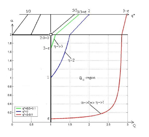
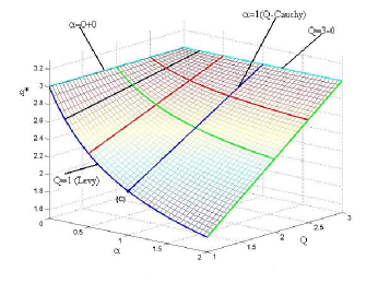
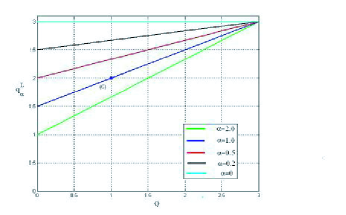
linking three parameters: Ξ±,𝛼\alpha, the parameter of the α𝛼\alpha-stable LΓ©vy distributions, q,π‘žq, the parameter of correlation, and qΞ±Lsubscriptsuperscriptπ‘žπΏπ›Όq^{L}_{\alpha}, the parameter of attractors in terms of qΞ±Lsubscriptsuperscriptπ‘žπΏπ›Όq^{L}_{\alpha}-Gaussians (see Fig. 2 (left)). Equation (38) identifies all (Q,Ξ±)𝑄𝛼(Q,\alpha)-stable distributions with the same index of attractor GqΞ±Lsubscript𝐺subscriptsuperscriptπ‘žπΏπ›ΌG_{q^{L}_{\alpha}} (See Fig. 1), proving the following proposition.

Proposition 6.6

Let 1≀Q<3,(Q=2​qβˆ’1)formulae-sequence1𝑄3𝑄2π‘ž11\leq Q<3,\,(Q=2q-1) and 0<Ξ±<2.0𝛼20<\alpha<2. Then all distributions Xβˆˆβ„’q​(Ξ±),𝑋subscriptβ„’π‘žπ›ΌX\in\mathcal{L}_{q}(\alpha), where the pairs (Q,Ξ±)𝑄𝛼(Q,\alpha) satisfy the equation

3+Q​αα+1=qΞ±L,3𝑄𝛼𝛼1superscriptsubscriptπ‘žπ›ΌπΏ\frac{3+Q\alpha}{\alpha+1}=q_{\alpha}^{L},

have the same attractor asymptotically equivalent to qΞ±Lsuperscriptsubscriptπ‘žπ›ΌπΏq_{\alpha}^{L}-Gaussian.

Refer to caption
Figure 1: All pairs of (Q,Ξ±)𝑄𝛼(Q,\alpha) on the indicated curves are associated with the same qΞ±Lsubscriptsuperscriptπ‘žπΏπ›Όq^{L}_{\alpha}-Gaussian. Two curves corresponding to two different values of qΞ±Lsuperscriptsubscriptπ‘žπ›ΌπΏq_{\alpha}^{L} do not intersect. In this sense these curves represent the constant levels of qΞ±Lsuperscriptsubscriptπ‘žπ›ΌπΏq_{\alpha}^{L} or Ξ·=2/(qΞ±Lβˆ’1).πœ‚2superscriptsubscriptπ‘žπ›ΌπΏ1\eta=2/(q_{\alpha}^{L}-1). The line Ξ·=1πœ‚1\eta=1 joins the points (Q,Ξ±)=(1,0.0βˆ’0)𝑄𝛼10.00(Q,\alpha)=(1,0.0-0) and (3βˆ’0,2)302(3-0,2); the line Ξ·=2πœ‚2\eta=2 joins the Cauchy distribution (noted C𝐢C) with itself at (Q,Ξ±)=(1,1)𝑄𝛼11(Q,\alpha)=(1,1) and at (2,2)22(2,2); the Ξ·=3πœ‚3\eta=3 line joins the points (Q,Ξ±)=(1,2.0βˆ’0)𝑄𝛼12.00(Q,\alpha)=(1,2.0-0) and (5/3,2)532(5/3,2) (by Ο΅italic-Ο΅\epsilon we simply mean to give an indication, and not that both infinitesimals coincide). The entire line at Q=1𝑄1Q=1 and 0<Ξ±<20𝛼20<\alpha<2 is mapped into the line at Ξ±=2𝛼2\alpha=2 and 5/3≀qβˆ—<353superscriptπ‘žβˆ—35/3\leq q^{\ast}<3.

In the particular case Q=1𝑄1Q=1, we recover the known connection between the classical LΓ©vy distributions (q=Q=1π‘žπ‘„1q=Q=1) and corresponding qΞ±Lsubscriptsuperscriptπ‘žπΏπ›Όq^{L}_{\alpha}-Gaussians. Put Q=1𝑄1Q=1 in Eq. (38) to obtain

qΞ±L=3+Ξ±1+Ξ±,  0<Ξ±<2.formulae-sequencesubscriptsuperscriptπ‘žπΏπ›Ό3𝛼1𝛼  0𝛼2q^{L}_{\alpha}=\frac{3+\alpha}{1+\alpha},\,\,0<\alpha<2. (39)

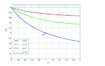
When α𝛼\alpha increases between 00 and 222 (i.e. 0<Ξ±<20𝛼20<\alpha<2), qΞ±Lsubscriptsuperscriptπ‘žπΏπ›Όq^{L}_{\alpha} decreases between 333 and 5/3535/3 (i.e. 5/3<qΞ±L<353subscriptsuperscriptπ‘žπΏπ›Ό35/3<q^{L}_{\alpha}<3): See Figs. 2 (left) and 3(left).

Refer to caption
Refer to caption
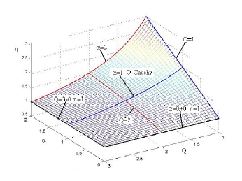
Figure 2: qΞ±L≑qβˆ—subscriptsuperscriptπ‘žπΏπ›Όsuperscriptπ‘žq^{L}_{\alpha}\equiv q^{*} and Ξ·πœ‚\eta as functions of variables (Q,Ξ±).𝑄𝛼(Q,\alpha).

It is useful to find the relationship between Ξ·=2qΞ±Lβˆ’1πœ‚2subscriptsuperscriptπ‘žπΏπ›Ό1\eta=\frac{2}{q^{L}_{\alpha}-1}, which corresponds to the asymptotic behaviour of the attractor depending on (Ξ±,Q)𝛼𝑄(\alpha,Q). Using formula (38), we obtain (Fig. 2, right)

Ξ·=2​(Ξ±+1)2+α​(Qβˆ’1).πœ‚2𝛼12𝛼𝑄1\eta=\frac{2(\alpha+1)}{2+\alpha(Q-1)}. (40)
Proposition 6.7

Let Xβˆˆβ„’Q​(Ξ±), 1≀Q<3, 0<Ξ±<2.formulae-sequenceformulae-sequence𝑋subscriptℒ𝑄𝛼1𝑄3 0𝛼2X\in\mathcal{L}_{Q}(\alpha),\,1\leq Q<3,\,0<\alpha<2. Then the associated density function fXsubscript𝑓𝑋f_{X} has asymptotics fX​(x)∼|x|Ξ·,|x|β†’βˆž,formulae-sequencesimilar-tosubscript𝑓𝑋π‘₯superscriptπ‘₯πœ‚β†’π‘₯f_{X}(x)\sim|x|^{\eta},\,|x|\rightarrow\infty, where Ξ·=η​(Q,Ξ±)πœ‚πœ‚π‘„π›Ό\eta=\eta(Q,\alpha) is defined in (40).

Remark 6.8

If Q=1𝑄1Q=1 (classic LΓ©vy distributions), then Ξ·=Ξ±+1πœ‚π›Ό1\eta=\alpha+1, as is well known.

Analogous relationships can be obtained for other values of Q𝑄Q. We call, for convenience, a (Q,Ξ±)𝑄𝛼(Q,\alpha)-stable distribution a Q𝑄Q-Cauchy distribution, if its parameter Ξ±=1.𝛼1\alpha=1. We obtain the classic Cauchy-Poisson distribution if Q=1𝑄1Q=1. The corresponding line can be obtained cutting the surface in Fig. 2 (right) along the line Ξ±=1𝛼1\alpha=1. For Q𝑄Q-Cauchy distributions we have

q1L​(Q)=3+Q2​and​η=4Q+1,subscriptsuperscriptπ‘žπΏ1𝑄3𝑄2andπœ‚4𝑄1q^{L}_{1}(Q)=\frac{3+Q}{2}\,\,\,\mbox{and}\,\,\,\eta=\frac{4}{Q+1}, (41)

respectively (see Figs. 2).

The relationship between α𝛼\alpha and qΞ±Lsubscriptsuperscriptπ‘žπΏπ›Όq^{L}_{\alpha} for typical fixed values of Q𝑄Q are given in Fig. 3 (left). In this figure we can also see, that Ξ±=1𝛼1\alpha=1 (Cauchy) corresponds to q1L=2subscriptsuperscriptπ‘žπΏ12q^{L}_{1}=2 (in the Q=1𝑄1Q=1 curve). In Fig. 3 (right) the relationships between Q𝑄Q (Q=2​qβˆ’1𝑄2π‘ž1Q=2q-1) and qΞ±Lsubscriptsuperscriptπ‘žπΏπ›Όq^{L}_{\alpha} are represented for typical fixed values of α𝛼\alpha.

Refer to caption
Refer to caption
Figure 3: Constant Q𝑄Q and constant α𝛼\alpha sections of Fig. 2(left).

We acknowledge thoughtful remarks by R. Hersh, E.P. Borges and S.M.D. Queiros. We thank E. Andries for his valuable assistance with MatLab codes and figures. Financial support by the Fullbright Foundation, SI International, AFRL and NIH grant P20 GMO67594 (USA agencies), and CNPq, Pronex and Faperj (Brazilian agencies) are acknowledged as well.

References

  • [1] S. Umarov, C. Tsallis and S. Steinberg, On a qπ‘žq-central limit theorem consistent with nonextensive statistical mechanics, Milan J. Math. 76 (2008) [DOI 10.1007/s00032-008-0087-y].
  • [2] C. Tsallis, Possible generalization of Boltzmann-Gibbs statistics, J. Stat. Phys. 52, 479 (1988). See also E.M.F. Curado and C. Tsallis, Generalized statistical mechanics: connection with thermodynamics, J. Phys. A 24, L69 (1991) [Corrigenda: 24, 3187 (1991) and 25, 1019 (1992)], and C. Tsallis, R.S. Mendes and A.R. Plastino, The role of constraints within generalized nonextensive statistics, Physica A 261, 534 (1998). A regularly updated bibliography is accessible at http://tsallis.cat.cbpf.br/biblio.htm
  • [3] D. Prato and C. Tsallis, Nonextensive foundation of Levy distributions, Phys. Rev. E 60, 2398 (1999), and references therein.
  • [4] M. Gell-Mann and C. Tsallis, eds., Nonextensive Entropy - Interdisciplinary Applications (Oxford University Press, New York, 2004).
  • [5] J.P. Boon and C. Tsallis, eds., Nonextensive Statistical Mechanics: New Trends, New Perspectives, Europhysics News 36 (6) (European Physical Society, 2005).
  • [6] C. Tsallis, Entropy, in Encyclopedia of Complexity and Systems Science (Springer, Berlin, 2008), in press.
  • [7] C. Tsallis, A.R. Plastino and R.F. Alvarez-Estrada, Escort mean values and the characterization of power-law-decaying probability densities, Archives 0802.1698 [cond-mat.stat-mech] (2008).
  • [8] B.V. Gnedenko, A.N. Kolmogorov, Limit Distributions for Sums of Independent Random Variables, 1954, Addison-Wesley, Reading.
  • [9] W. Feller, An Introduction to Probability Theory and its Applications II, John Wiley and Sons, Inc, New York and London and Sydney, 1966
  • [10] G. Samorodnitsky and M.S. Taqqu, Stable non-Gaussian Random Processes, Chapman and Hall , New York, 1994.
  • [11] V.V. Uchaykin and V.M. Zolotarev, Chance and Stability. Stable Distributions and their Applications, VSP, Utrecht, 1999.
  • [12] M.M. Meerschaert, H.-P. Scheffler, Limit Distributions for Sums of Independent Random Vectors. Heavy Tails in Theory and Practice, John Wiley and Sons, Inc, 2001.
  • [13] G. Zaslavsky, Chaos, fractional kinetics, and anomalous transport. Physics Reports (2002), 371, 461-580.
  • [14] C. Beck and F. Schloegel, Thermodynamics of Chaotic Systems: An Introduction (Cambridge University Press, Cambridge, 1993).
  • [15] R. Metzler and J. Klafter, The random walk’s guide to anomalous diffusion: a fractional dynamics approach, Physics Reports, Physics Reports, 339, 1, 2000, 1 .
  • [16] R. Gorenflo and F. Mainardi and D. Moretti and G. Pagnini and P. Paradisi, Discrete random walk models for space-time fractional diffusion, Chemical Physics 284, 521 (2002).
  • [17] M.M. Meerschaert, H.-P. Scheffler, Limit theorems for continuous-time random walk with infinite mean waiting times. J. Appl. Probability 41, 623 (2004).
  • [18] F.G. Schmitt, L. Seuront, Multifractal Random Walk in Copepod Behavior, Physica A 301, 375 (2001).
  • [19] G. Jona-Lasinio, The renormalization group: A probabilistic view, Nuovo Cimento B 26, 99 (1975), and Renormalization group and probability theory, Phys. Rep. 352, 439 (2001), and references therein; P.A. Mello and B. Shapiro, Existence of a limiting distribution for disordered electronic conductors, Phys. Rev. B 37, 5860 (1988); P.A. Mello and S. Tomsovic, Scattering approach to quantum electronic transport, Phys. Rev. B 46, 15963 (1992); M. Bologna, C. Tsallis and P. Grigolini,Anomalous diffusion associated with nonlinear fractional derivative Fokker-Planck-like equation: Exact time-dependent solutions, Phys. Rev. E 62, 2213 (2000); C. Tsallis, C. Anteneodo, L. Borland and R. Osorio, Nonextensive statistical mechanics and economics, Physica A 324, 89 (2003); C. Tsallis, What should a statistical mechanics satisfy to reflect nature?, in Anomalous Distributions, Nonlinear Dynamics and Nonextensivity, eds. H.L. Swinney and C. Tsallis, Physica D 193, 3 (2004); C. Anteneodo, Non-extensive random walks, Physica A 358, 289 (2005); S. Umarov and R. Gorenflo, On multi-dimensional symmetric random walk models approximating fractional diffusion processes, Fractional Calculus and Applied Analysis 8, 73-88 (2005); S. Umarov and S. Steinberg, Random walk models associated with distributed fractional order differential equations, to appear in IMS Lecture Notes - Monograph Series; F. Baldovin and A.L. Stella, Central limit theorem for anomalous scaling due to correlations, Phys. Rev. E 75, 020101 (2007); C. Tsallis, On the extensivity of the entropy Sqsubscriptπ‘†π‘žS_{q}, the qπ‘žq-generalized central limit theorem and the qπ‘žq-triplet, in Complexity and Nonextensivity: New Trends in Statistical Mechanics, eds. S. Abe, M. Sakagami and N. Suzuki, Prog. Theor. Phys. Suppl. 162, 1 (2006); D. Sornette, Critical Phenomena in Natural Sciences (Springer, Berlin, 2001), page 36.
  • [20] C. Tsallis and D.J. Bukman, Anomalous diffusion in the presence of external forces: exact time-dependent solutions and their thermostatistical basis, Phys. Rev. E 54, R2197 (1996).
  • [21] S. Abe and A.K. Rajagopal, Rates of convergence of non-extensive statistical distributions to LΓ©vy distributions in full and half-spaces, J. Phys. A 33, 8723 (2000).
  • [22] C. Tsallis, Nonextensive statistical mechanics, anomalous diffusion and central limit theorems, Milan Journal of Mathematics 73, 145 (2005).
  • [23] L.G. Moyano, C. Tsallis and M. Gell-Mann, Numerical indications of a qπ‘žq-generalised central limit theorem, Europhys. Lett. 73, 813 (2006); H.J. Hilhorst and G. Schehr, A note on qπ‘žq-Gaussians and non-Gaussians in statistical mechanics, J. Stat. Mech. (2007) P06003; A. Rodriguez, V. Schwammle and C. Tsallis, Strictly and asymptotically scale-invariant probabilistic models of N𝑁N correlated binary random variables having qπ‘žq-Gaussians as Nβ†’βˆžβ†’π‘N\to\infty limiting distributions, Archives 0804.1488 [cond-mat.stat-mech] (2008).
  • [24] C. Tsallis, What are the numbers that experiments provide ?, Quimica Nova 17, 468 (1994).
  • [25] C. Tsallis and S.M.D. Queiros, Nonextensive statistical mechanics and central limit theorems I - Convolution of independent random variables and qπ‘žq-product, in Complexity, Metastability and Nonextensivity, eds. S. Abe, H.J. Herrmann, P. Quarati, A. Rapisarda and C. Tsallis, American Institute of Physics Conference Proceedings 965, 8-20 (New York, 2007).
  • [26] S.M.D. Queiros and C. Tsallis, Nonextensive statistical mechanics and central limit theorems II - Convolution of qπ‘žq-independent random variables, in Complexity, Metastability and Nonextensivity, eds. S. Abe, H.J. Herrmann, P. Quarati, A. Rapisarda and C. Tsallis, American Institute of Physics Conference Proceedings 965, 21-33 (New York, 2007).
  • [27] E.P. Borges, A q-generalization of circular and hyperbolic functions, J. Phys. A: Math. Gen. 31 (1998), 5281-5288.
  • [28] L. Nivanen, A. Le Mehaute and Q.A. Wang, Generalized algebra within a nonextensive statistics, Rep. Math. Phys. 52, 437 (2003).
  • [29] E.P. Borges, A possible deformed algebra and calculus inspired in nonextensive thermostatistics, Physica A 340, 95 (2004).
  • [30] C. Tsallis, M. Gell-Mann and Y. Sato, Asymptotically scale-invariant occupancy of phase space makes the entropy Sqsubscriptπ‘†π‘žS_{q} extensive, Proc. Natl. Acad. Sc. USA 102, 15377 (2005).
  • [31] J. Marsh and S. Earl, New solutions to scale-invariant phase-space occupancy for the generalized entropy Sqsubscriptπ‘†π‘žS_{q}, Phys. Lett. A 349, 146 (2005).
  • [32] C. Tsallis, M. Gell-Mann and Y. Sato, Extensivity and entropy production, Europhysics News 36, 186 (2005).
  • [33] J.A. Marsh, M.A. Fuentes, L.G. Moyano and C. Tsallis, Influence of global correlations on central limit theorems and entropic extensivity, Physica A 372, 183 (2006).