Entanglement and Bell States in Superconducting Flux Qubits

Abstract

We theoretically study macroscopic quantum entanglement in two superconducting flux qubits. To manipulate the state of two flux qubits, a Josephson junction is introduced in the connecting loop coupling the qubits. Increasing the coupling energy of the Josephson junction makes it possible to achieve relatively strong coupling between the qubits, causing two-qubit tunneling processes to be even dominant over the single-qubit tunneling processes in the states of two qubits. It is shown that due to the two-qubit tunneling processes both the ground state and excited states of the coupled flux qubits can be a Bell type state, maximally entangled, in experimentally accessible regimes. The parameter regimes for the Bell states are discussed in terms of magnetic flux and Josephson coupling energies.

Introduction.$-$ Quantum entanglement is a fundamental resource for quantum information processing and quantum computing Nielsen . Numerous proposals have been made for the creation of entanglement in solid-state systems: quantum dots Glazman ; Marcus ; Engel ; Piermarocchi , Kondo impurities Cho , carbon nanotubes Ardavan and so on. For superconducting qubits coherent manipulation of quantum states in a controllable manner has enabled to generate partially entangled states Pashkin ; Berkley ; Izmalkov . However, in realizing such quantum technologies, highly entangled quantum states such as the Bell states of two qubits are required Nielsen . Of particular importance, therefore, are the preparation and measurement of such maximally entangled states.

Recently, several types of superconducting qubits have been demonstrated experimentally. In superconducting qubits experimental generations of entanglements have been reported for coupled charge qubits Pashkin and coupled phase qubits Berkley , but the maximally entangled Bell states is far from experimental realization as yet. This paper aims to answer on how maximally entangled states can be prepared by manipulating system parameters in solid-state qubits. We quantify quantum entanglement in the two superconducting flux qubits based on the phase-coupling scheme. In this study we show that, if the coupling strength between two flux qubits is strong enough, simultaneous two-qubit coherent tunneling processes make it possible to create a maximally entangled state in the ground and excited states. Furthermore, it is shown that the ranges of system parameters for a maximally entangled state are sufficiently wide that a Bell-type state should be realizable experimentally. Actually, a coherent two-qubit flipping processes has been experimentally observed in inductively coupled flux qubits Izmalkov . However, the strength of the inductive coupling Majer is too weak to achieve a maximally entangled state.

Figure 1: Left and right superconducting loops are connected each other by a connecting loop interrupted by a Josephson junction. The state of each qubit loop is the superposed state of the diamagnetic and paramagnetic current states assigned by $\left|\downarrow\right\rangle$ and $\left|\uparrow\right\rangle$, respectively, which can make the loop being regarded as a qubit. For example, the state, $\left|\downarrow\uparrow\right\rangle$, out of four possible basis of two-qubit current states is shown, where the arrows indicate the flow of Cooper pairs and thus in reverse direction is the current. Here, $\odot$ (oppositely $\otimes$) denote the directions of the magnetic fields, $f_{L(R)}=\Phi_{L(R)}/\Phi_{0}$, in the qubit loops. $E_{J1}$, $E_{J}$, and $E^{\prime}_{J}$ are the Josephson coupling energies of the Josephson junctions in the qubit loops and the connecting loop and $\phi$’s are phase differences across the Josephson junctions.

We use a phase-coupling scheme Kim to obtain sufficiently strong coupling and show a maximally entangled state between two flux qubits. Very recently, this phase-coupling scheme has been realized in an experiment Ploeg using two four-junctions flux qubits. To theoretically study a controllable coupling manner in the flux qubits, the phase coupling scheme has also been employed KimCC ; Grajcar . Further, there have been studies about somewhat different types of phase-coupling schemes Grajcar3 ; Brink . The phase-coupling scheme for two flux qubits (See Fig. 1) is to introduce a connecting loop interrupted by a Josephson junction in order to couple two three-junctions qubits Mooij ; Kim1 . In the connecting loop, the Josephson energy depends on the phase difference, $\phi_{L1}-\phi_{R1}$, and the coupling energy, $E^{\prime}_{J}$, of the junction. As varies $E^{\prime}_{J}$, the coupling strength between the flux qubits, defined by the energy difference between the same direction current state and the different direction current state in the two flux qubits, can be increased to be relatively strong. The coupling strength between the phase-coupled flux qubits is a monotonously increasing function of $E^{\prime}_{J}$ Kim .

For small $E_{J}^{\prime}(\ll E_{J})$, the effective potential for the two qubits has a symmetric form in the phase variable space. Then single-qubit tunneling processes in the two qubit states are predominant in the effective potential. They have almost the same tunneling amplitudes. The eigenstates are nearly degenerate at the operating point of the external fluxes so that the entanglement between two qubits is very weak. As increases the Josephson coupling energy, $E_{J}^{\prime}$, the shape of the effective potential is deformed to be a less symmetric form. Then the amplitudes of single-qubit tunneling processes are decreased. However, the deformation of the effective potential allows a two-qubit tunneling process not negligible and even dominant over the single-qubit tunneling processes. We will then derive explicitly the contribution of two-qubit tunneling processes. To generate a Bell type of maximally entangled state, the two-qubit tunneling processes are shown to play an important role.

Model.$-$ Let us start with the charging energy of the Josephson junctions: $E_{C}=\frac{1}{2}\left(\Phi_{0}/2\pi\right)^{2}(\sum^{3}_{i=1}(C_{Li}\dot{\phi}^{2}_{Li}+C_{Ri}\dot{\phi}^{2}_{Ri})+C^{\prime}\dot{\phi^{\prime}}^{2})$, where $C_{L(R)i}$ and $C^{\prime}$ are the capacitance of the Josephson junctions for the left (right) qubit loop and the connecting loop, respectively. Here, $\phi$’s are the phase differences across the Josephson junctions and $\Phi_{0}\equiv h/2e$ the superconducting unit flux quantum. Since the number of excess Cooper pair charges on the Josephson junctions, $\hat{N_{i}}\equiv\hat{Q}_{i}/2e$ with $Q_{i}=C(\Phi_{0}/2\pi){\dot{\phi}_{i}}$, is conjugate to the phase difference $\hat{\phi}_{i}$ such as $[\hat{\phi}_{i},\hat{N_{i}}]=i$, the canonical momentum, $\hat{P}_{i}\equiv\hat{N_{i}}\hbar=-i\hbar\partial/\partial\hat{\phi}_{i}$, can be introduced. Then the Hamiltonian is given by

$$\hat{H}=\frac{1}{2}\hat{P}^{T}_{i}{M}^{-1}_{ij}\hat{P}_{j}+U_{\rm eff}(\hat{\bm{\phi}}),$$ (1)

where $M_{ij}=(\Phi_{0}/2\pi)^{2}C_{i}\delta_{ij}$ is the effective mass and $\hat{\bm{\phi}}=(\phi_{L1},\phi_{L2},\phi_{L3},\phi_{R1},\phi_{R2},\phi_{R3},\phi^{\prime})$. If we neglect the small inductive energy, the effective potential becomes the energy of the Josephson junctions such as $U_{\rm eff}(\bm{\phi})=\sum^{3}_{i=1}E_{Ji}(1-\cos\phi_{Li})+\sum^{3}_{i=1}E_{Ji}(1-\cos\phi_{Ri})+E^{\prime}_{J}(1-\cos\phi^{\prime})$.

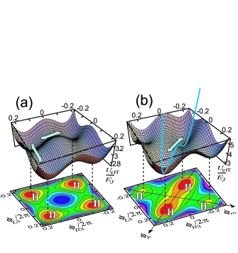
Figure 2: (Color online) The effective potential of Eq. (2) for the coupled flux qubits at the co-resonance point $f_{L}=f_{R}=0.5$ as a function of $\phi_{L3}$ and $\phi_{R3}$ with $E_{J1}=0.7E_{J}$. In the contour plots of the effective potential, the four local minima correspond to the current states of the coupled flux qubits: $\left|\uparrow\uparrow\right\rangle,\left|\uparrow\downarrow\right\rangle,\left|\downarrow\uparrow\right\rangle$, and $\left|\downarrow\downarrow\right\rangle$. The left-right arrows ($\Longleftrightarrow$) on the effective potential profiles indicate some of single-/two-qubit tunneling processes (For example, $\left|\downarrow\uparrow\right\rangle\Longleftrightarrow\left|\uparrow\uparrow\right\rangle$ and $\left|\downarrow\downarrow\right\rangle\Longleftrightarrow\left|\uparrow\uparrow\right\rangle$, respectively). (a) For $E^{\prime}_{J}=0$, the four local minima of the effective potential have nearly the same energies. The potential barrier of the double well for a two-qubit tunneling process are much wider and higher than the potential barriers for the single-qubit tunneling processes. Thus, single-qubit tunneling processes are dominant and the entanglement is very weak. (b) For $E^{\prime}_{J}=0.6E_{J}$, only $\left|\downarrow\uparrow\right\rangle$ and $\left|\uparrow\downarrow\right\rangle$ are lifted up to a higher energy while $\left|\uparrow\uparrow\right\rangle$ and $\left|\downarrow\downarrow\right\rangle$ stay at the same energies. Then the potential barrier for the two-qubit tunneling process between $\left|\downarrow\downarrow\right\rangle$ and $\left|\uparrow\uparrow\right\rangle$ is not changed so much that the tunneling amplitude also is not changed. An asymmetric double well potential for single-qubit tunneling processes makes the tunneling amplitude decreasing as $E_{J}^{\prime}$ increases. Therefore, the two-qubit tunneling process plays a significant role on the entanglement of the coupled flux qubits.

Since the qubit operations are performed experimentally at near the co-resonance point, we can set $f_{L}=f_{R}=0.5$ with $f_{L(R)}\equiv\Phi_{L(R)}/\Phi_{0}$ and the total flux $\Phi_{L(R)}$ threading the left (right) qubit loop. In experiments, the two Josephson junctions with phase differences, $\phi_{L(R)2}$ and $\phi_{L(R)3}$, are considered nominally the same so that it is reasonable to set $E_{J2}=E_{J3}=E_{J}$ and $\phi_{L(R)2}=\phi_{L(R)3}$. Furthermore, if one can neglect the small inductive flux, the boundary conditions in the left and right qubit loops and the connecting loop are given approximately, $2\pi(n_{L(R)}+f_{L(R)})-(\phi_{L(R)1}+\phi_{L(R)2}+\phi_{L(R)3})=0$ and $2\pi r+(\phi_{L1}-\phi_{R1})-\phi^{\prime}=0$ with integers $n_{L},n_{R}$ and $r$. Introducing the rotated coordinates with $\phi_{p}\equiv(\phi_{L3}+\phi_{R3})/2$ and $\phi_{m}\equiv(\phi_{L3}-\phi_{R3})/2$, the Hamiltonian can be rewritten in the form, ${\hat{H}}={\hat{P}}_{p}^{2}/2M_{p}+{\hat{P}}_{m}^{2}/2M_{m}+U_{\rm eff}(\hat{\phi}_{p},\hat{\phi}_{m}),$ where the effective potential becomes

$$U_{\rm eff}(\phi_{p},\phi_{m})=2E_{J1}(1+\cos 2\phi_{p}\cos 2\phi_{m})~{}~{}~{}~{}~{}~{}~{}~{}~{}~{}$$ (2)

$$+4E_{J}(1-\cos\phi_{p}\cos\phi_{m})+E^{\prime}_{J}(1-\cos 4\phi_{m}).$$

Here, $M_{p}\equiv\hbar^{2}(2C_{1}+C)/e^{2}$, $M_{m}\equiv\hbar^{2}(2C_{1}+C+4C^{\prime})/e^{2}$ and the conjugate momentum is $\hat{P}_{p(m)}=-i\hbar\partial/\partial\hat{\phi}_{p(m)}$ with commutation relation, $[\hat{\phi}_{p(m)},\hat{P}_{p(m)}]=i\hbar$.

We display the effective potential as a function of $\phi_{L3}$ and $\phi_{R3}$ in Fig. 2. The effective potential is shown to have the four local potential minima corresponding to the four states of the coupled qubits, i.e., $\left|\uparrow\uparrow\right\rangle,\left|\uparrow\downarrow\right\rangle,\left|\downarrow\uparrow\right\rangle$, and $\left|\downarrow\downarrow\right\rangle$. At the local minima of the effective potential, one can obtain the energy levels: $E_{ss^{\prime}}=(1/2)\hbar(\omega_{p,ss^{\prime}}+\omega_{m,ss^{\prime}})+U_{\rm eff}(\phi_{p,ss^{\prime}},\phi_{m,ss^{\prime}})$, where $s,s^{\prime}=1/2$ and $-1/2$ stand for spin up, $\left|\uparrow\right\rangle$, and spin down, $\left|\downarrow\right\rangle$, respectively. In the harmonic oscillator approximation Orlando , the characteristic oscillating frequencies, $\omega_{p(m),ss^{\prime}}$, are given by $\omega_{p(m),ss^{\prime}}=(k_{p(m),ss^{\prime}}/M_{p(m)})^{1/2}$ with $k_{p(m),ss^{\prime}}\equiv\partial^{2}U_{\rm eff}(\phi_{p},\phi_{m})/\partial\phi^{2}_{p(m)}|_{(\phi_{p,ss^{\prime}},\phi_{m,ss^{\prime}})}$, where $\phi_{p,ss^{\prime}}(\phi_{m,ss^{\prime}})$ are the values of $\phi_{p}(\phi_{m})$ at the local potential minimum. Then the tight-binding approximation gives the Hamiltonian in the basis, $\{\left|\uparrow\uparrow\right\rangle,\left|\uparrow\downarrow\right\rangle,\left|\downarrow\uparrow\right\rangle,\left|\downarrow\downarrow\right\rangle\}$, as follows;

$$H\!\! = \!\!\!\!\!\!\sum_{s,s^{\prime}=\pm\frac{1}{2}}E_{ss^{\prime}}|s,s^{\prime}\rangle\langle s,s^{\prime}|+H^{T}_{1}+H^{T}_{2},$$ (3)

$$H^{T}_{1}\!\! = \!\!\!\!\!\!\sum_{s,s^{\prime}=\pm\frac{1}{2}}\!\!\Big{(}-t^{L}_{1}|s,s^{\prime}\rangle\langle-s,s^{\prime}|-t^{R}_{1}|s,s^{\prime}\rangle\langle s,-s^{\prime}|\Big{)},$$ (4)

$$H^{T}_{2}\!\! = \!\!\!\sum_{s=\pm\frac{1}{2}}\Big{(}-t^{a}_{2}|s,s\rangle\langle-s,-s|-t^{b}_{2}|s,-s\rangle\langle-s,s|\Big{)},$$ (5)

where $H^{T}_{1(2)}$ describe the single(two)-qubit tunneling processes between the two-qubit states with the tunneling amplitudes $t^{L,R}_{1}$($t^{a,b}_{2}$). Normally, the single-qubit tunneling amplitudes are much larger than the two-qubit tunneling amplitudes, i.e., $t^{a,b}_{2}\ll t^{L,R}_{1}$. Thus, the two-qubit tunneling Hamiltonian $H^{T}_{2}$ can be neglected when $E_{J}^{\prime}$=0.

Two-qubit tunnelings and entanglements.$-$ For the weak coupling limit, $E_{J}^{\prime}\ll E_{J}$, the single-qubit tunnelings between the two-qubit states can be obtained by the tunnelings in the well-behaved double well potentials as shown as left-right arrows in Fig. 2(a). As increases $E_{J}^{\prime}$, the well-behaved double well potentials for the single-qubit tunnelings become an asymmetric double well potentials shown clearly in Fig. 2(b). Then the asymmetry of the double well potentials makes the single-qubit tunneling amplitudes decrease drastically. However, as the blue line shown in Fig. 2(b), the corresponding double well potential to the two-qubit tunneling between the states $\left|\uparrow\uparrow\right\rangle$ and $\left|\downarrow\downarrow\right\rangle$ is not changed much qualitatively. Actually, from the effective potential in Eq. (2), the double well potential is given by

$$U_{\rm eff}(\phi_{p},0)=2E_{J1}(1+\cos 2\phi_{p})+4E_{J}(1-\cos\phi_{p}).$$ (6)

The two-qubit tunneling amplitudes $t^{a}_{2}$ between the states $\left|\uparrow\uparrow\right\rangle$ and $\left|\downarrow\downarrow\right\rangle$ is written in the WKB approximation Orlando ,

$$\!\!\!\!\!\!\!t^{a}_{2}\!\!\! = \!\!\!\frac{\hbar\omega_{p,ss}}{2\pi}\exp\!\!{\left[\!-\sqrt{\frac{2M_{p}}{\hbar^{2}}}\!\int\!\!d\phi_{p}\sqrt{U_{\rm eff}(\phi_{p},0)-E_{ss}}\right]}.$$ (7)

Here $M_{p}$, $\omega_{p,ss}$ and $U_{\rm eff}(\phi_{p},0)$ do not depend on the capacitance, $C^{\prime}$, and the Josephson coupling energy, $E^{\prime}_{J}$, of the Josephson junction in the connecting loop. Equation (7) shows that the two-qubit tunneling amplitude remains unchanged even though $E^{\prime}_{J}$ is increased. As a consequence, the two-qubit tunneling between the states $\left|\uparrow\uparrow\right\rangle$ and $\left|\downarrow\downarrow\right\rangle$ in Hamiltonian $H^{T}_{2}$ of Eq. (5) will play a crucial role to improve the entanglement between the coupled flux qubits.

For $E_{J}^{\prime}=0$, we obtain the tunneling amplitudes; $t^{L,R}_{1}\approx 0.0075E_{J}$ and $t^{a}_{2}=t^{b}_{2}\approx 0.00024E_{J}$ with $E_{J1}=0.7E_{J}$. As expected, $t^{a,b}_{2}\ll t^{L,R}_{1}$ and the two-qubit tunneling terms of the Hamiltonian are negligible. When $E^{\prime}_{J}\neq 0$, in order to get the single-qubit tunneling amplitudes between an asymmetric double well potentials, the Fourier Grid Hamiltonian Method Marton is employed because the WKB approximation cannot be applicable in the asymmetric double well potential. For $E_{J}^{\prime}=0.6E_{J}$ as shown in Fig. 2(b), we obtain the tunneling amplitudes of $t^{L,R}_{1}\approx 10^{-5}E_{J}$ and $t^{a}_{2}\approx 0.00024E_{J}$. Here, the tunneling amplitude $t^{b}_{2}$ is neglected because the the wave function overlap between the states $\left|\uparrow\downarrow\right\rangle$ and $\left|\downarrow\uparrow\right\rangle$ is negligible in Fig. 2(b).

One measure of entanglement is the concurrence, ${\cal C}$, for an arbitrary state of coupled two qubits. The concurrence ranges from 0 for nonentangled to 1 for maximally entangled states. For a normalized pure state, $\left|\psi\right\rangle=a\left|\downarrow\downarrow\right\rangle+b\left|\uparrow\downarrow\right\rangle+c\left|\downarrow\uparrow\right\rangle+d\left|\uparrow\uparrow\right\rangle$, the concurrence Wootters is given by

$${\cal C}(\left|\psi\right\rangle)=2\left|ad-bc\right|.$$ (8)

We evaluate the concurrence in Eq. (8) numerically to show that a maximally entangled state is possible in the ground state by varying the Josephson coupling energy in the connecting loop. In Fig. 3(a), we plot the concurrence for the ground state, ${\cal C}(\left|\psi_{G}\right\rangle)$, of the Hamiltonian in Eqs. (3)$-$(5) as a function of $f_{p(m)}=(f_{L}\pm f_{R})/2$ for $E_{J}^{\prime}=0.6E_{J}$ and $E_{J1}=0.7E_{J}$. A broad ridge of the concurrence along the line $f_{p}=0.5$ shows a high entanglement between the two qubits. This region corresponds to the central part of the honeycomb type potential of coupled qubits in Ref. Kim, near the co-resonance point, $f_{L}=f_{R}=0.5$. Away from the co-resonance point we can numerically calculate concurrences without using the analytic effective potential in Eq. (2) obtained by introducing a few approximations Kim . Figure 3(b) shows the cut view of the concurrence at $f_{p}=0.5$ (dotted line in Fig. 3(a)) as a function of $f_{m}$ for various values of $E_{J}^{\prime}$. For $E^{\prime}_{J}=0.005E_{J}$, corresponding to the coupling strength of inductively coupled qubits in the experiment of Ref. Majer, , a partial entanglement can only exist around $f_{m}\sim 0$. As increases $E_{J}^{\prime}$, i.e., when the two-qubit tunneling becomes dominant over the single-qubit tunneling, a maximum entanglement appears. In Fig. 3(c), we display the coefficients of the ground state wavefunction, $\left|\psi_{G}\right\rangle=a(f_{m})\left|\downarrow\downarrow\right\rangle+b(f_{m})\left|\uparrow\downarrow\right\rangle+c(f_{m})\left|\downarrow\uparrow\right\rangle+d(f_{m})\left|\uparrow\uparrow\right\rangle$, as a function of $f_{m}$ for $E^{\prime}_{J}=0.2E_{J}$. We see the ground state wavefunction:

$$\left|\psi_{G}\right\rangle\simeq\!\left\{\begin{array}[]{ll}\left|\downarrow\uparrow\right\rangle&\mbox{for $f_{m}\lesssim-0.04$}\\ \!\!\!\displaystyle\frac{1}{\sqrt{2}}\left(\left|\downarrow\downarrow\right\rangle+\left|\uparrow\uparrow\right\rangle\right)&\mbox{for $-0.04\lesssim f_{m}\lesssim 0.04$}\\ \left|\uparrow\downarrow\right\rangle&\mbox{for $f_{m}\gtrsim 0.04$}\\ \end{array}\right.\!\!.$$ (12)

This ground state has the Bell type of maximally entangled state, $|\Phi^{+}\rangle=(\left|\downarrow\downarrow\right\rangle+\left|\uparrow\uparrow\right\rangle)/\sqrt{2}$, for $-0.04\lesssim f_{m}\lesssim 0.04$. Similarly, one can see that the 1st excited state shows, actually, another Bell type of maximally entangled state, $\left|\Phi^{-}\right\rangle=(\left|\downarrow\downarrow\right\rangle-\left|\uparrow\uparrow\right\rangle)/\sqrt{2}$.

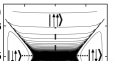
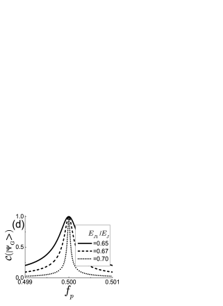
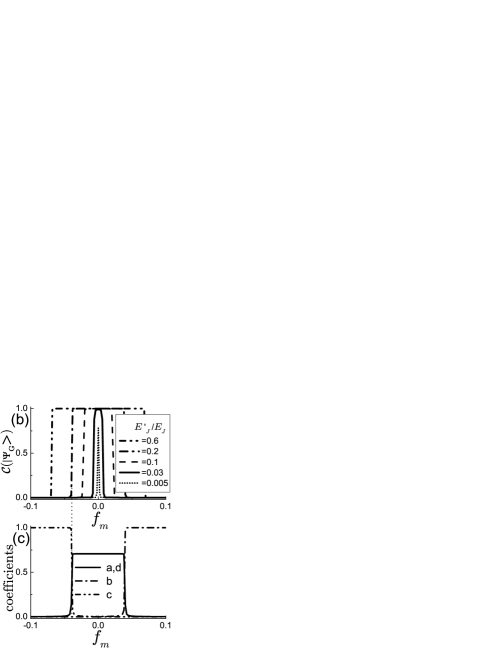
Figure 3: (a) Concurrence for the ground state of the coupled flux qubits as a function of $f_{p(m)}=(f_{L}\pm f_{R})/2$ for $E^{\prime}_{J}=0.6E_{J}$ and $E_{J1}=0.7E_{J}$. A high entanglement between two flux qubits is seen in the broad ridge with $f_{p}=0.5$. In the contour plot, $\left|\downarrow\downarrow\right\rangle$, $\left|\uparrow\downarrow\right\rangle$, $\left|\downarrow\uparrow\right\rangle$, and $\left|\uparrow\uparrow\right\rangle$ denote the coupled-qubit states located far from the co-resonance point, $f_{L}=f_{R}=0.5$. (b) Concurrences for various $E^{\prime}_{J}$ along the line of $f_{p}=0.5$ (dotted line in (a)) for $E_{J1}=0.7E_{J}$. As increases $E^{\prime}_{J}$, the maximum entanglement appears for $E^{\prime}_{J}\gtrsim 0.03\,E_{J}$. (c) The coefficients of the ground state wavefunction, $\left|\psi_{G}\right\rangle=a(f_{m})\left|\downarrow\downarrow\right\rangle+b(f_{m})\left|\uparrow\downarrow\right\rangle+c(f_{m})\left|\downarrow\uparrow\right\rangle+d(f_{m})\left|\uparrow\uparrow\right\rangle$, as a function of $f_{m}$ for the case $E^{\prime}_{J}=0.2E_{J}$ in (b). For $-0.04\lesssim f_{m}\lesssim 0.04$, the Bell type of maximally entangled state, $|\Phi^{+}\rangle=(\left|\downarrow\downarrow\right\rangle+\left|\uparrow\uparrow\right\rangle)/\sqrt{2}$, is shown clearly because $a=d=1/\sqrt{2}$ and $b=c=0$. (d) Concurrences for various $E_{J1}$ along the line of $f_{m}=0$ for $E^{\prime}_{J}=0.6E_{J}$ (dashed line in (a)). As decreases $E_{J1}$, since the two-qubit tunneling amplitude increases, the width of concurrence peak becomes so wide that the maximal entanglement should be observable experimentally.

The cut view of the concurrence at $f_{m}=0$ (dashed line in (a)) is shown in Fig. 3(d) for various $E_{J1}$ with $E^{\prime}_{J}=0.6E_{J}$. As $E_{J1}$ increases, the barrier of the double well potential in Eq. (6) becomes higher. Thus the two-qubit tunneling amplitude, $t^{a}_{2}$, decreases such that $t^{a}_{2}/E_{J}\approx$ 0.0016, 0.0008, 0.00024 for $E_{J1}/E_{J}$=0.65, 0.67, 0.7, respectively. In Fig. 3(d), as a result, the width of the concurrence peak becomes narrower, which will make an experimental implementation of the maximum entanglement difficult. On the other hand, if the value of $E_{J1}$ becomes much smaller than $E_{J1}=0.65E_{J}$, the barrier of double well potential can be lower than the ground energy of the harmonic potential wells, $E_{ss}$, and the two-qubit states, $\left|\downarrow\downarrow\right\rangle$ and $\left|\uparrow\uparrow\right\rangle$, in Fig. 2(b) will not be stable. In addition, as seen in Fig. 3(b), the range of $E^{\prime}_{J}$ for maximal entanglement is approximately $E_{J}^{\prime}\gtrsim 0.03E_{J}$. Therefore, for a maximally entangled state of the two flux qubits, it is required that $E_{J1}$ should be controlled around $0.7E_{J}$ with $E^{\prime}_{J}\gtrsim 0.03\,E_{J}$.

For $E^{\prime}_{J}\ll E_{J}$, the concurrence is very small because the four states are nearly degenerated due to the weak coupling between the qubits and $t^{L,R}_{1}\gg t^{a,b}_{2}$. As $E^{\prime}_{J}$ increases, the coupling between the qubits is much stronger and $t^{a}_{2}$ becomes much dominant over than other tunneling processes, $t^{L}_{1}$, $t^{R}_{1}$, and $t^{b}_{2}$. In a strong coupling limit, $t^{L}_{1},t^{R}_{1},t^{b}_{2}\ll t^{a}_{2}$ and $E_{s,s}<E_{s,-s}$. If we with the split energies, $E_{\downarrow\downarrow}=E_{0}-\delta E$ and $E_{\uparrow\uparrow}=E_{0}+\delta E$ around the co-resonance point. $f_{L}=f_{R}\approx 0.5$ Then the concurrence of the ground state is given by ${\cal C}(\left|\psi_{G}\right\rangle)\simeq|t^{a}_{2}/\sqrt{(t^{a}_{2})^{2}+(\delta E)^{2}}|$, which corresponds to the behaviors in Fig. 3(d). At the co-resonance point ($f_{L}=f_{R}=0.5$), the ground state is in a maximally entangled state, i.e., ${\cal C}(\left|\psi_{G}\right\rangle)=1$. This shows the important role of the two-qubit tunneling process making the two qubits entangled and maintaining the highly entangled state against fluctuations of $f_{L,R}$ away from the co-resonance point as long as $\delta E\lesssim t^{a}_{2}$.

Summary.$-$ We studied the entanglement to achieve a maximally entangled state in a coupled superconducting flux qubits. A Josephson junction in the connecting loop coupling the two qubits was employed to manipulate the qubit states. As increases the Josephson coupling energy of the Josephson junction, the two-qubit tunneling processes between the current states play an important role to make the two flux qubit strongly entangled. It was shown that a Bell type of maximally entangled states can be realized in the ground and excited state of the coupled qubit system. We also identified the system parameter regime for the maximally entangled states.

Acknowledgments. We thank Yasunobu Nakamura for helpful discussions. This work was supported by the Ministry of Science & Technology of Korea (Quantum Information Science) and the Australian Research Council.

References

(1)
M. Nielsen and I. Chuang,
Quantum Computation & Quantum Information
(Cambridge University Press, Cambridge, 2000).
(2)
L. I. Glazman and R. C. Ashoori, Science 304, 524 (2004).
(3) N. J. Craig et al.,
Science 304, 565 (2004).
(4)
H.-A. Engel and D. Loss,
Science 309, 586 (2005).
(5) C. Piermarocchi et al.,
Phys. Rev. Lett. 89, 167402 (2002).
(6)
S. Y. Cho and R. H. McKenzie,
Phys. Rev. A 73, 012109 (2006).
(7)
A. Ardavan et al.,
Phil. Trans. R. Soc. Lond. A 361, 1473 (2003).
(8) Yu. A. Pashkin et al.,
Nature 421, 823 (2003).
(9) A. J. Berkley et al.,
Science 300, 1548 (2003).
(10) A. Izmalkov et al.,
Phys. Rev. Lett. 93, 037003 (2004).
(11) J. B. Majer et al.,
Phys. Rev. Lett. 94, 090501 (2005).
(12) M. D. Kim and J. Hong, Phys. Rev. B 70, 184525 (2004).
(13) S. H. W. van der Ploeg et al.,
cond-mat/0605588.
(14) M. D. Kim, cond-mat/0602604.
(15) M. Grajcar et al.,
cond-mat/0605484.
(16) M. Grajcar et al., Phys. Rev. Lett. 96, 047006 (2006).
(17) A. Maassen van den Brink, cond-mat/0605398.
(18) J. E. Mooij et al.,
Science 285, 1036 (1999);
Caspar H. van der Wal et al.,
Science 290, 773 (2000);
I. Chiorescu et al.,
Nature 431, 138 (2004).
(19) M. D. Kim et al.,
Phys. Rev. B 68, 134513 (2003).
(20) T. P. Orlando et al.,
Phys. Rev. B 60, 15398 (1999).
(21) C. C. Marton and G. G. Balint-Kurti, J. Chem. Phys.
91, 3571 (1989).
(22) W. K. Wootters, Phys. Rev. Lett. 80, 2245 (1998);
S. Hill and W. K. Wootters, Phys. Rev. Lett. 78, 5022 (1997).